 Channa Rajanayaka1*
 Simon J. R. Woodward2†
 Linda Lilburne3Sam Carrick3
 James Griffiths1M. S. Srinivasan1
 Christian Zammit1Jesús Fernández-Gálvez4
- 1National Institute of Water and Atmospheric Research Limited, Christchurch, New Zealand
- 2National Institute of Water and Atmospheric Research Limited, Hamilton, New Zealand
- 3Manaaki Whenua—Landcare Research Limited, Lincoln, New Zealand
- 4Department of Regional Geographic Analysis and Physical Geography, University of Granada, Granada, Spain
Hydrological modeling for landscape and catchment scale applications requires upscaling of soil hydraulic parameters which are generally only available at point scale. We present a case study where hourly root zone soil water content and drainage observations from nine flat, pastoral sites (Waikato and Canterbury regions in New Zealand) were used to develop an upscaling approach to parameterize the soil water balance module of the TopNet catchment model, based on scaling multi-layer soil profile information from the national soil data base, S-map, to the single-layer soil profile used in TopNet. Using a Bayesian calibration approach, the hydraulic behavioral parameters of TopNet's soil water balance module were identified. Of the eleven calibration parameters considered three were found to be insensitive to data (stress point, unsaturated hydraulic conductivity and infiltration rate); three were correlated and could be determined from specific soil water content observations (wilting point, field capacity and drainable water); and five were correlated and could be determined from combined specific soil water content and drainage observations (drainage rate, saturated hydraulic conductivity profile, effective soil depth, soil water holding capacity and wetting front suction). Based on the eight correlated parameters, upscaling functions were then developed to derive suitable model parameters from S-map-hydro for each site. The validity of the upscaling functions was verified at each site. The approach used in this research can be used to parameterize the TopNet model at other similar locations, and also provides a transferable framework to parameterize other catchment-scale hydrology models where point-scale soil hydraulic data available.
Highlights
- Point-scale soil hydraulic parameters can be upscaled using soil water state and flux data.
- Bayesian calibration allows prior information to be combined with uncertainty in the model input.
- A simple upscaling scheme was developed to estimate representative model parameters from the high-resolution point scale observations, using inverse modeling.
- The upscaled parameters produce seasonal patterns and annual totals of water fluxes, but do not match uncalibrated soil water content measurements.
Introduction
Water is one of the fundamental resources required for food production, and is frequently the resource that limits production, either because crop water demand exceeds water supply from rain and/or irrigation, or because agricultural activities that adversely affect water quality (e.g., effluent application) are tightly regulated (FAO, 2011; MfE, 2021). Understanding and optimizing the availability and use of water to grow crops requires accurate knowledge of water supply, use and loss that can be used to estimate water availability, particularly soil water content, at a suitable scale for management and policy decisions (Vereecken et al., 2007; Curk and Glavan, 2021). TopNet is one such tool (Bandaragoda et al., 2004; Clark et al., 2008) that has been developed by National Institute of Water and Atmospheric Research (NIWA, New Zealand) to link spatial rainfall and irrigation supply, with water use at catchment scale, to aquifer, stream, river and lake hydrology up to a national scale. Although TopNet has been successfully used in several national studies (McMillan et al., 2013; Griffiths et al., 2021), its accuracy at catchment scale is currently limited by the scale of data available on soil properties. The national S-map data set (MWLR, 2022) provides soil survey polygons that are linked to point-scale soil properties for up to six layers down to a maximum of 1 m depth from surface. As soil-water hydraulic parameters greatly vary with spatial scale (Bresler and Dagan, 1983; Gelhar, 1986; Gómez-Hernández and Gorelick, 1989; Flury et al., 1994; Iversen et al., 2001), the S-map soil data need to be scaled vertically as well as laterally for use in TopNet. The objective of the current work focuses on the first task which is to develop a scheme by which the detailed multi-layer point-scale soil properties from S-map could be vertically upscaled for use in the single-layer TopNet model. This upscaling of detailed vertical soil profile data will also have application in other hydrological and agricultural models currently in use in New Zealand and elsewhere.
Several approaches exist for parameter upscaling. In this paper, the differences between field observations and the model simulated outputs are used to infer the scale and selection of parameters to be estimated, using an inverse upscaling method (Šimunek and Van Genuchten, 1996; Abbaspour et al., 1997; Lehmann and Ackerer, 1997; Zhang et al., 2000a,b, 2003; Ward et al., 2006; Pollacco et al., 2022b). The inverse method of Bayesian calibration in particular is used, which allows prior information to be combined with uncertainty in the model input, model parameters, model structure, and calibration data, and also quantifies the resulting predictive uncertainty. However, associated numerical methods, such as Markov Chain Monte Carlo (MCMC) sampling, are numerically demanding, and their use is consequently limited to relatively fast models with few parameters (e.g., Schoups and Vrugt, 2010; Li et al., 2012; Jiang et al., 2015). An overview of the history of MCMC methods is provided by Wu and Zeng (2013), leading up to the development of the Differential Evolution Adaptive Metropolis algorithm, DREAM (Vrugt et al., 2009), a variant of which (DREAMZS) is used in this study (Ter Braak and Vrugt, 2008).
Aims
The S-map-hydro database within the New Zealand digital national soil database (S-map) holds soil-hydraulic data (Lilburne et al., 2012). However, the database contains more spatial and vertical detail than is generally required by catchment models. The overarching aim of this study is to develop a method for upscaling multilayer vertical soil-hydraulic parameters for use in less vertically detailed modeling and analysis. Here upscaling refers to simplifying the high resolution (multi-layer) soil information into a low resolution (single layer) in accordance with the hydrological model requirements.
The approach taken in this study was to develop a simple upscaling technique for S-map-hydro soil water parameters to use in the single soil-layer TopNet model (Bandaragoda et al., 2004; Clark et al., 2008). This preliminary upscaling scheme was developed with data from flat, grass pasture sites. Extension to other sites, soils, and vegetation types will require additional testing. The scaling method is depicted in Figure 1.
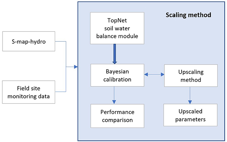
Figure 1. Conceptual model for upscaling soil hydraulic properties.
Materials and methods
The S-map and S-map-hydro databases
S-map is a digital, multi-layer soil database that was developed to capture soil survey information describing soil variability down to 1 m depth, along with the associated uncertainty (Lilburne et al., 2012). S-map-hydro is an extension of S-map (Lilburne et al., 2012, 2014; McNeill et al., 2018). S-map-hydro provides data for describing the soil water retention θ(ψ) (Kosugi, 1994, 1996), and unsaturated hydraulic conductivity K(θ) functions (Pollacco et al., 2017, 2022a; Fernández-Gálvez et al., 2021), for up to six functional horizons to a maximum depth of 100 cm, for a 150 × 150 m spatial grid. Vertical soil data is provided for 14 fixed depth layers (2.5, 5, 10, 15, 20, 25, 30, 40, 50, 60, 70, 80, 90, and 100 cm) across much of New Zealand.
Point-scale soil water balance model
To assess the extent to which soil hydraulic parameters provided by S-map-hydro can be used effectively in a parsimonious soil hydrology and catchment model, a point-scale soil water balance submodule from the distributed hydrological model TopNet (version 10) (Bandaragoda et al., 2004; Clark et al., 2008) was parameterised for case study soil types in Waikato and Canterbury regions of New Zealand. TopNet is a single layer (tipping bucket) catchment-scale rainfall-runoff model built on the concepts of TOPMODEL (Beven and Kirkby, 1979; Beven et al., 1995). TopNet uses sub-surface water storage to control the dynamics of saturation excess runoff and baseflow recession.
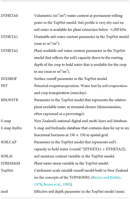
The parameters of the point-scale soil water balance submodule of TopNet model are listed in Table 1. Canopy moisture parameters represent a very small portion of the water balance at the grazed pasture study sites, so were set to fixed values. An exponential hydraulic conductivity profile option was used [TOPMODF parameter (Beven et al., 1995)] so the TOPMODM and TOPMODN parameters were not needed. The TOPMODEL subbasin slope ratio parameter ALAMBDA (Bandaragoda et al., 2004; Clark et al., 2008) was also not required for the point-scale water balance model used here. The remaining parameters were calibrated within the ranges shown in Table 1, assuming a symmetrical beta-distribution prior. The following parameters control the soil water content range: DTHETA0, DTHETA2, DTHETA1, SOILCAP. In theory, DTHETA0 corresponds to permanent wilting point, below which water cannot be extracted by plants (ostensibly −1,500 kPa); DTHETA2 represents plant available water, theoretically the difference between field capacity (−10 kPa) and permanent wilting point; DTHETA1 represents water content in the soil above field capacity up to saturation (0 kPa); and SOILCAP corresponds to water content within the soil column, which equates to effective soil depth times (DTHETA1 + DTHETA2). RPAWSTR controls plant soil water stress response; HYDCON0, CH_CEXP, and TOPMODF control the drainage response; GA_PSIF controls the surface runoff response; and the initial conditions are defined by SOILH2O and ZBARH2O.
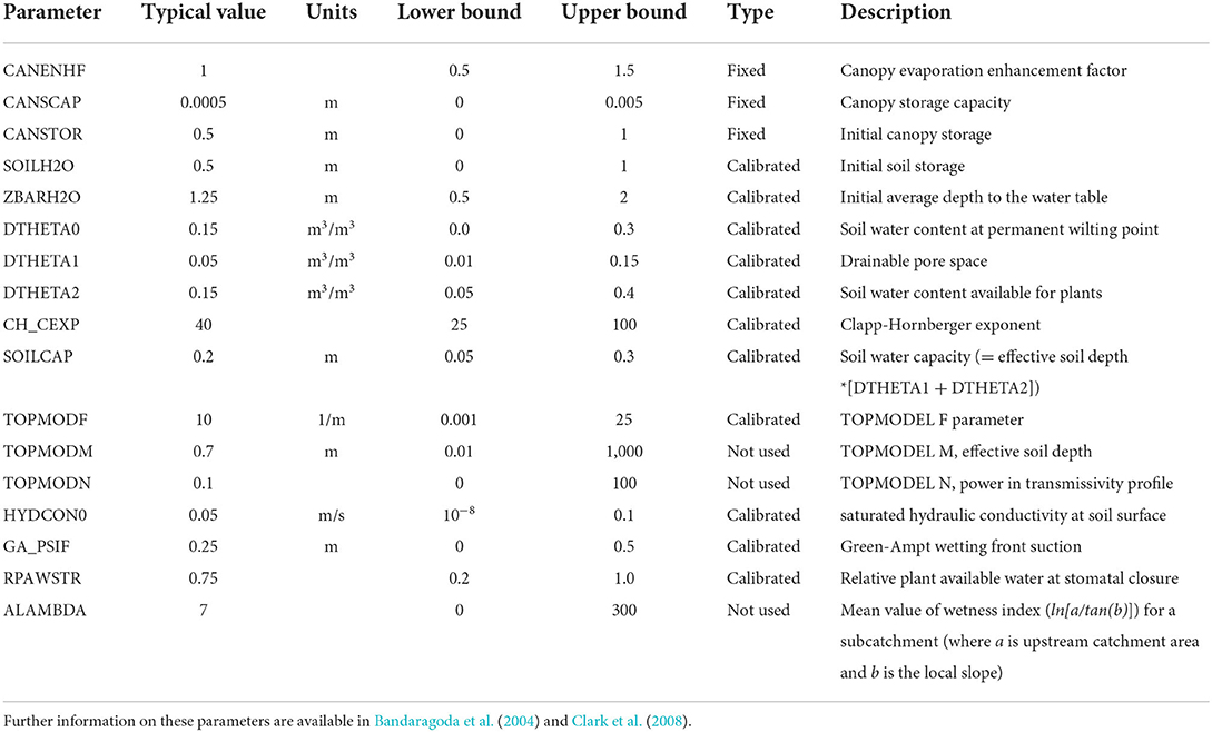
Table 1. TopNet soil water balance module parameters.
Case study sites
High resolution soil moisture data were collated from nine field monitoring sites with contrasting soil types, five in the Waikato region of New Zealand's North Island, and four in the Canterbury region of New Zealand's South Island (Figure 2). Site climate data is summarized in Table 2. The Waikato sites are dryland pasture sites and were monitored with tipping bucket rain gauges, and supplemented with hourly potential evapotranspiration values (the latter stochastically-disaggregated from daily values from the National Institute of Water and Atmospheric Research's (NIWA) virtual climate station network (VCSN) (Tait et al., 2006). No drainage measurements were made at the Waikato sites. The Canterbury sites were irrigated pastures and were monitored with tipping bucket rain gauges and lysimeters to 70 cm depth as described in Duncan et al. (2016).
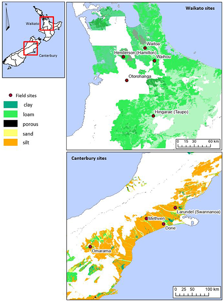
Figure 2. Location of Canterbury and Waikato field sites. Canterbury: four irrigated sites (soil water content and lysimeters) at Methven, Dorie, Larundel (Swannanoa), and Omarama. Waikato: five non-irrigated sites (soil moisture only) at Waihou, Otorohanga, Hingarae (Taupo), Henderson (Hamilton), and Waitoa.
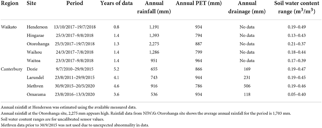
Table 2. Summary of climate and soil water content data at case study sites.
Surface runoff was not measured at any of the sites, but all sites were located on flat terrains. Rubber collars were placed on the lysimeters to prevent flow from entering or leaving the lysimeter surface at the Canterbury sites. Surface runoff was therefore assumed to be nominally zero at all sites.
Soils were selected to represent both being spatially extensive in each case study area, as well as a range in key soil attributes, as summarized in Table 3.
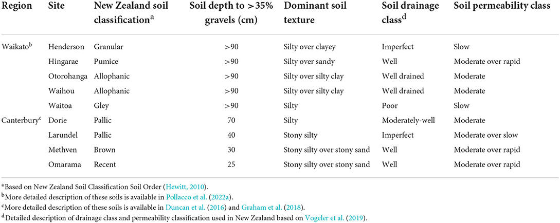
Table 3. Summary of soil classification and key features at each site.
Waikato sites
Details of the five Waikato sites are presented in Table 4. Soil sampling has been collected for five horizons, and in the laboratory dry bulk density (for three sites only) and water contents at 0, −5, −10, −20, −40, −100, and −1,500 kPa were determined (McLeod et al., 2015, 2016). At each site, five Decagon 5TM (www.decagon.com) soil moisture sensors have been installed at depths to coincide with soil horizons, from 5.5 to 100 cm below ground level.
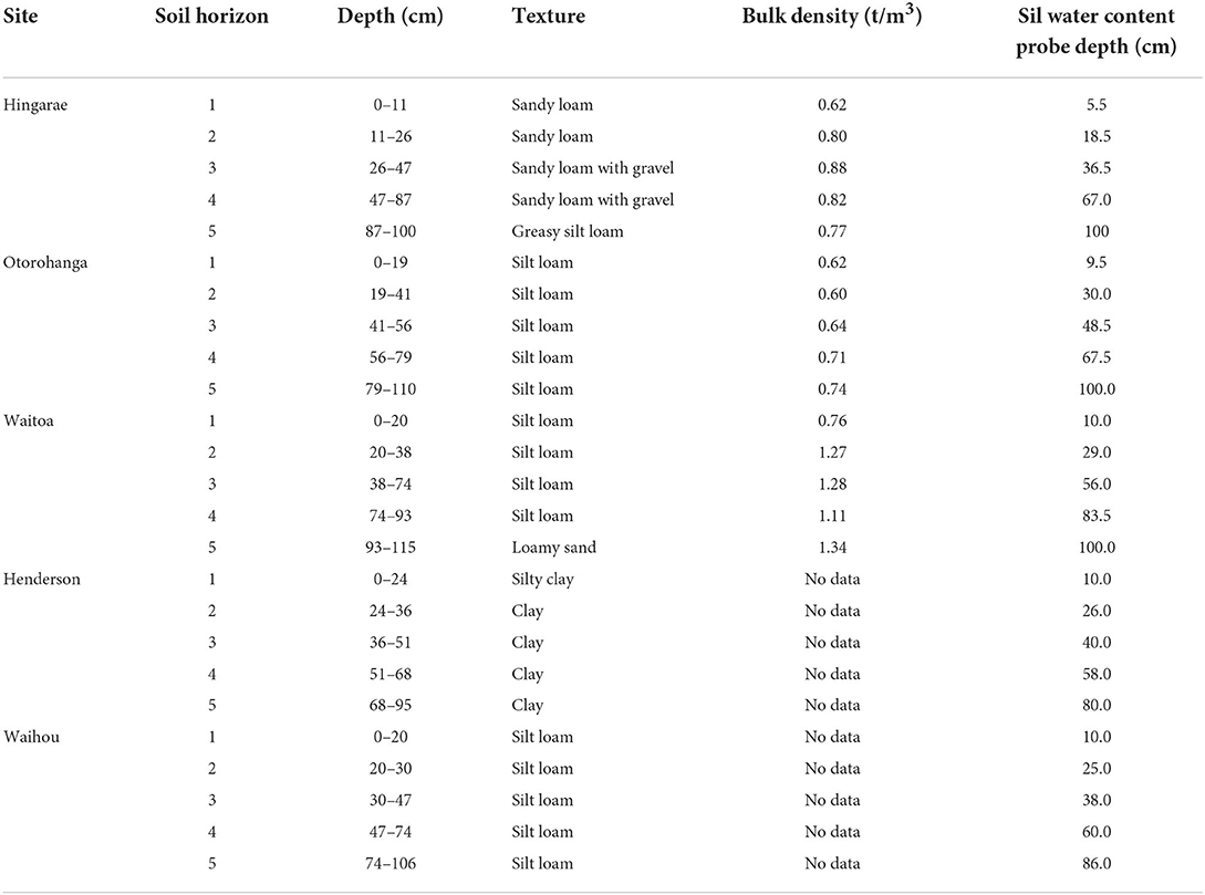
Table 4. Soil and soil water content probe information at Waikato sites.
The ground cover at all sites is ryegrass/white clover dominated pasture. All five sites are unirrigated.
Canterbury sites
The study sites in Canterbury were selected to represent a range of soils and management regimes. Unlike Waikato sites, all Canterbury sites are spray irrigated regularly between the months of October and April. Time domain transmissometry (TDT, www.acclima.com) soil water content sensors were installed at up to three depths (varying from 9.5 to 70 cm below ground level). Soil and TDT soil water content probes information are listed in Table 5, and Figure 3 shows a schematic of the instrument layout at the lysimeter sites.
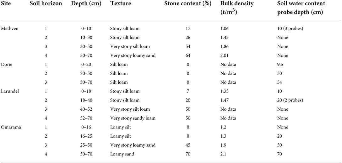
Table 5. Soil and soil water content probe information at Canterbury sites.
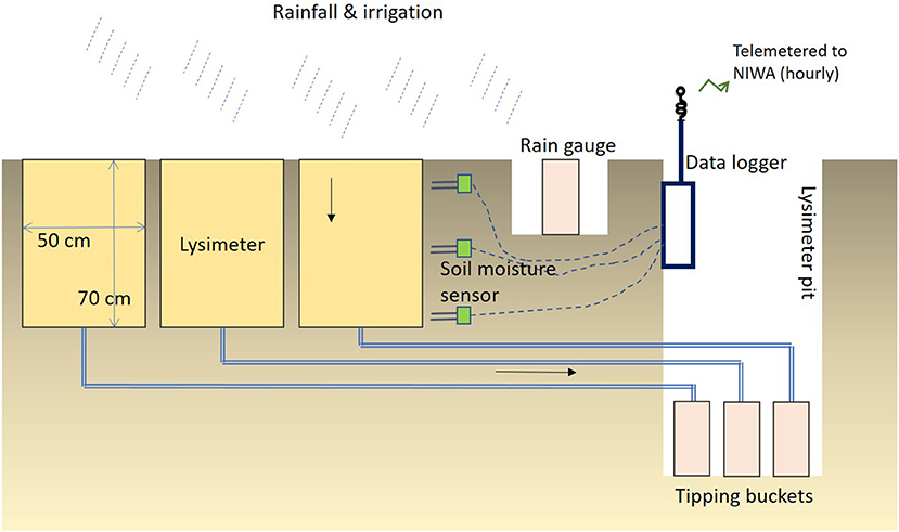
Figure 3. Schematic of lysimeter instrument (Source: Duncan et al., 2016).
Similar to the Waikato sites, land cover at the Canterbury sites is ryegrass/white clover dominated pasture. For all sites, the lysimeters represent soil water movement correctly with respect to capillary rise. Maximum groundwater levels at Methven and Dorie for example are 39 and 6 m below the surface, respectively, so the water table is too deep for to have any capillary rise effect on those lysimeters (Duncan et al., 2016).
Each lysimeter site consists of three cylindrical, non-weighing, drainage lysimeters 0.5 m in diameter and 0.7 m in depth (similar dimensions to those in White et al., 2003).
Data preparation
For each site, the soil water content, drainage, rainfall, and potential evapotranspiration (PET) data were aggregated (or in case of potential evapotranspiration, disaggregated from daily values) into hourly data, to match the simulation time step of TopNet. The units of the data were volume of water over a volume of soil (m3/m3) for the soil water content data (see following paragraph) and mm/h for drainage, rainfall and PET.
Soil water content measurements based on TDT and 5TM sensors are considered uncalibrated. Although neutron probe measurements were available for calibration, this is not straightforward, due to the infrequency of the measurements. The accuracy of neutron probe measurements close to the soil-air interface is generally low due to the fact that the sphere of influence (radius) of the neutron probe instrument extends into the air above the soil surface (Chanasyk and Naeth, 1996), and neutron probe data themselves were not calibrated with in situ measurements. For this reason, the uncalibrated soil water content data was used for model calibration, with the understanding that the soil water content data represent trends rather than absolute values (Srinivasan et al., n.d.). In addition, the daily difference in mean soil water content over successive days (see Section Soil water content measurements and tension profiles) was used an additional data set for model calibration. Experience shows that in calibration, daily soil water content time series information primarily infers the seasonal patterns of soil water content, while the fine detail of soil water response to rain or irrigation events is poorly reproduced. Including the difference as an additional calibration variable allows the calibration to more accurately infer the parameters controlling the daily response.
The soil water content time series at the different sites are shown in Figure 4. Sensors closer to the surface (e.g., at 55, 95, or 100 mm below the surface) often had extremely dynamic (flashy) signals, presumably due to short term ponding and infiltration lags, whereas sensors below 100 mm tended to have much subdued variation.
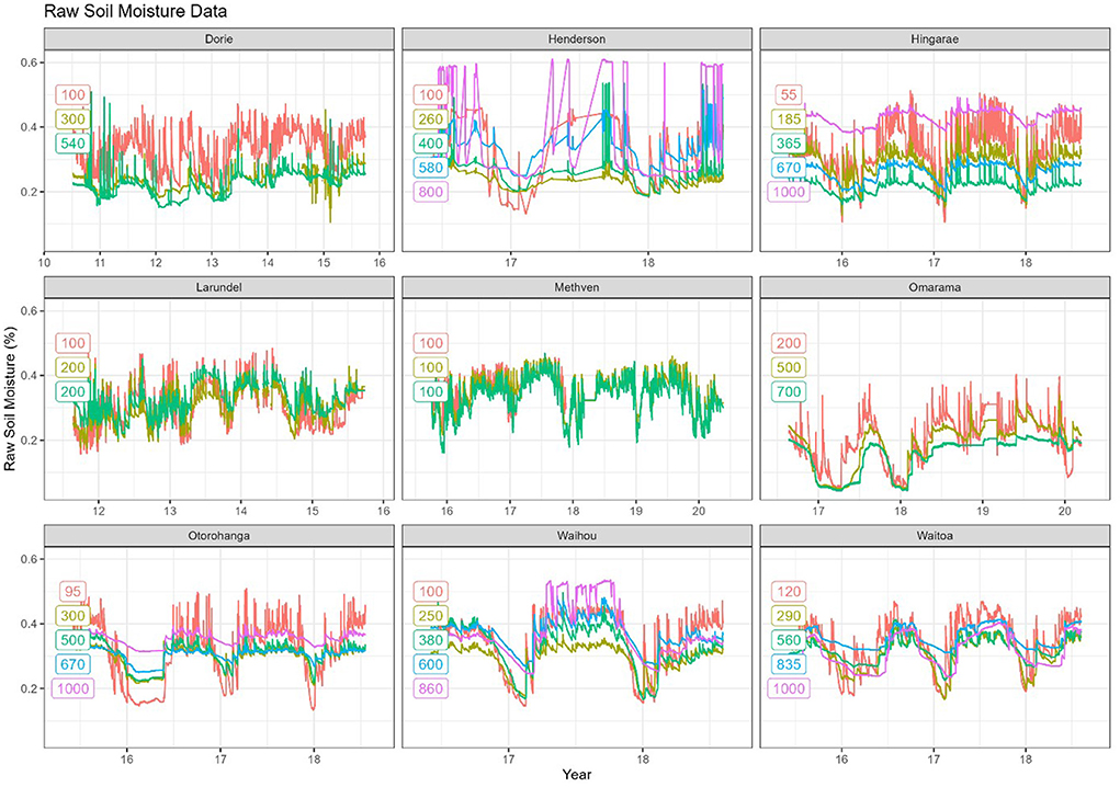
Figure 4. Soil water content data at each site. Sensor depths (mm) are shown as colored labels.
The various configurations of soil water content sensors at the different sites made it difficult to establish a consistent approach across sites for summarizing the multi-sensor soil water content data into a single hourly value. The Waikato sites had five sensors down to about 1,000 mm, whereas several of the Canterbury sites only had very shallow sensors (due to the shallow topsoil and stony subsoil). Furthermore, the shallowest sensors at each site often had extremely dynamic data. To achieve a consistent approach, only data from near-surface soil water content sensor from the surface was used for model calibration to identify behavioral parameter sets. As a result, for the Waikato sites, the second sensor was used (located at depths ranging from 185 mm at Hingarae to 300 mm at Otorohanga). For the Canterbury sites, the hourly average soil water content from all sensors no deeper than 300 mm were used.
Model calibration
The purpose of model calibration was to establish what model parameter sets were consistent with the measured field data. This was done by adjusting the model parameters until the model simulations match the observed field data. The field data to be matched should reflect the desired use of the model. In the current study, we wish to use the TopNet soil water balance model primarily to predict surface runoff, plant water stress, and drainage (in order to drive a catchment scale hydrological model).
Calibration was performed using aggregated (daily) data. This was the temporal resolution of the climate data (other than precipitation) used to drive the TopNet model (stochastically downscaled to an hourly time step), and a suitable time step for matching the model predictions to the drainage data, since in TopNet excess water drains immediately (within an hourly timestep) but drainage occurs gradually in the monitored data. No surface runoff observation data were available, but all of the soils were deemed to likely have sufficient infiltration capacity, so surface runoff was calibrated against a nominal value of 0 mm. Drainage was only measured and used for calibration at the Canterbury sites.
Model calibration at each site was carried out following the Bayesian calibration method described in Woodward et al. (2020). Bayesian calibration identifies the distribution of parameter sets for which the observed data have a high likelihood of having occurred. The likelihood is conditioned by prior assumptions about the parameter ranges. The resulting (“posterior”) parameter sets express the uncertainty of the calibration and can be used to make model predictions including uncertainty bounds.
The prior parameter ranges used for TopNet calibration are given in Table 1. The model was calibrated to four observation time series at each site: daily mean soil water content (m3/m3), difference in daily mean soil water content over successive days (m3/m3/d), daily total drainage (mm/d), where available, and daily total surface runoff (mm/d) (assumed to be always zero). The standard errors of these measurements (, , , , respectively) were assumed to be 0.02, 0.005, 1.0, and 1.0. Autocorrelation between the daily measurements was discounted by weighting the likelihood components with equal weights (ws, wc, wd, wr, respectively) of 1/30. It is assumed that the residuals are not autocorrelated on a monthly (30 day) time scale (see Schoups and Vrugt, 2010), following Woodward et al. (2017).
The log-likelihood (LL) was then calculated as:
where:
• ws, wc, wd, and wr are weights (all equal to 1/30) to account for auto-correlation between the residuals,
• ns, nc, nd, and nr are the number of hourly observations for soil water content (s), soil water content change (c), drainage (d), and surface runoff (r), respectively,
• , and , are the soil water content observations (o), model predictions (m), and errors (e), respectively,
• , and , are the soil moisture change observations (o), model predictions (m), and errors (e), respectively,
• , , and are the soil drainage observations (o), model predictions (m), and errors (e), respectively,
• , , and are the surface runoff observations (o), model predictions (m), and errors (e), respectively, and
• f(z) is the log probability density function (Student's-t distribution with 7 degrees of freedom, see Woodward et al., 2020).
Calibration was carried out using BayesianTools (Hartig et al., 2019) package in R (R Core Team, 2022) with three independent DREAMZS chains run in parallel (each containing three internal chains that give nine Markov chains in total) in increments of 10,000 samples, until the Gelman-Rubin MCMC convergence statistic (Gelman and Rubin, 1992) was below 1.1 for all parameters. The last 10,000 samples from each of the nine chains were then combined and taken as the posterior distribution. The maximum a posteriori (MAP) parameter set was also recorded, which is the parameter set corresponding to the mode of the posterior, and can be thought of as the parameter set giving the best fit to the data and the prior (with the caveat that the other posterior parameter sets may be quite different, and yet give a fit that is almost as good). Plots were prepared using the ggplot2 package (Wickham, 2016) in R.
Model performance evaluation
Model calibration performance was summarized by calculating two measures of goodness of fit: root-mean-squared error (RMSE), which is the standard deviation of the residuals, and the Nash-Sutcliffe model efficiency (NSE) (Nash and Sutcliffe, 1970), which is the proportion of the variation in the data which is explained by the model. RMSE is measured in the same units as the data and can be compared directly to the assumed standard errors in Equation (1): if the RMSE is much smaller than the standard errors of the data this indicate overfitting, and if the RMSE is much larger than the standard errors of the data this indicates underfitting. NSE is a more popular measure of goodness of fit (being a generalization of the coefficient of determination, R2) but is more difficult to interpret. This is because NSE depends on the variation in the data, whereas RMSE does not. NSE tends to be high when the variation in the data is high, and low when the variation in the data is low, regardless of model performance. NSE values therefore cannot be compared across different data series.
Scaling S-map parameters
Following model calibration (Section Model calibration), parameter upscaling was done based on data from the soil parameter database S-map-hydro. This data was obtained by using the field descriptions of the nine sites to enter nine site-specific soil siblings into the S-map database. Pedo-transfer functions were used to derive the estimates of water content at seven tensions (McNeill et al., 2018). By fitting a Kosugi curve to these estimates, other hydrological parameters can be derived, e.g., hydraulic conductivity at saturation, Green-Ampt and other TopNet parameters in Table 1 (Green and Ampt, 1911; Pollacco et al., 2017). These soil parameters were extracted for each of the nine sites at the 14 fixed depths described in Section The S-map and S-map-hydro databases.
As described earlier, most soil water models for catchment or regional scale application are not designed to use such high-resolution data. These parameters must therefore be simplified (“upscaled”) for application to larger scale simulations. Following model calibration, the posterior distributions of the model parameters (shown in Table 1) were compared with the S-map-hydro parameters for the sites. Due to the small number of sites, a simple upscaling relationship was developed to estimate suitable TopNet parameters from the S-map-hydro parameters (by matching the parameter distributions derived during model calibration to the field data). This upscaling scheme was based on data from flat, pastoral sites only, and is provisional contingent on further validation in future. In principle, the upscaling relationship can then be used to derive suitable model parameters for other sites and allow TopNet to be applied more widely to sites where high-resolution time series data are not available.
Results
Soil water content measurements and tension profiles
The soil water content-tension profiles for the nine sites in the current study are shown in Figure 5 alongside laboratory measurements made on cores. Superimposed on these parameters and data are violin plots showing the soil water content data ranges from the current study (by depth in blue, and as summarized in black).
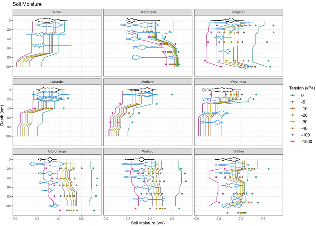
Figure 5. Soil water content ranges with depth, comparing the uncalibrated soil water content probes (Figure 4, blue violin plots), with the S-map-hydro parameter database (lines), and laboratory measurements (dots). The black violin plots show the range of soil water content data used for model calibration, as described in the text.
In general, the lab measurements of soil water content match the S-map-hydro parameters at these sites, although there are exceptions. In some cases, the 0 kPa (saturated) points did not match well, and the range between −10 and 0 kPa seems large. Since the S-map-hydro parameters were estimated based on pedo-transfer functions from laboratory data, it is not surprising that they might be inaccurate under saturated conditions. The soil water content sensor data are generally in the ranges expected from the S-map-hydro database and lab measurements (the nominal range generally quoted for field conditions is −1,500 to −10 kPa), however they are often in the >-10 kPa range (drainable porosity) at Dorie, Larundel, and Methven. At other sites the values are too low (near or below −1,500 kPa) which should rarely happen in the field, e.g., Henderson, Otorohanga, Waihou, and Waitoa.
Fit to data
The calibrated model successfully reproduced the observed patterns of soil water content and drainage data for all data sets. For example, the fit to the Methven data is shown in Figure 6 (fits for other field sites along with their results are provided in the Appendix). The four plots show soil water content (SOILM), drainage (DRAINGE), surface runoff (INXSROF) and plant water stress (STRESSMM), respectively. In each sub-plot, red traces show the observed data (where available), blue shows the calibrated model traces, and gray shows the simulation based on the upscaled parameter values (derived as explained in Section Upscaling of soil hydraulic parameters). The large numbers on the left of each plot gives the average values of observed data, calibrated model and upscaled parameter model, in red, blue, and gray, respectively. We desire that the model faithfully reproduces the seasonal patterns of SOILM, DRAINAGE, INXSROF and STRESSMM data, as well as the annual totals (apart from the average SOILM value, since the sensor data was uncalibrated).
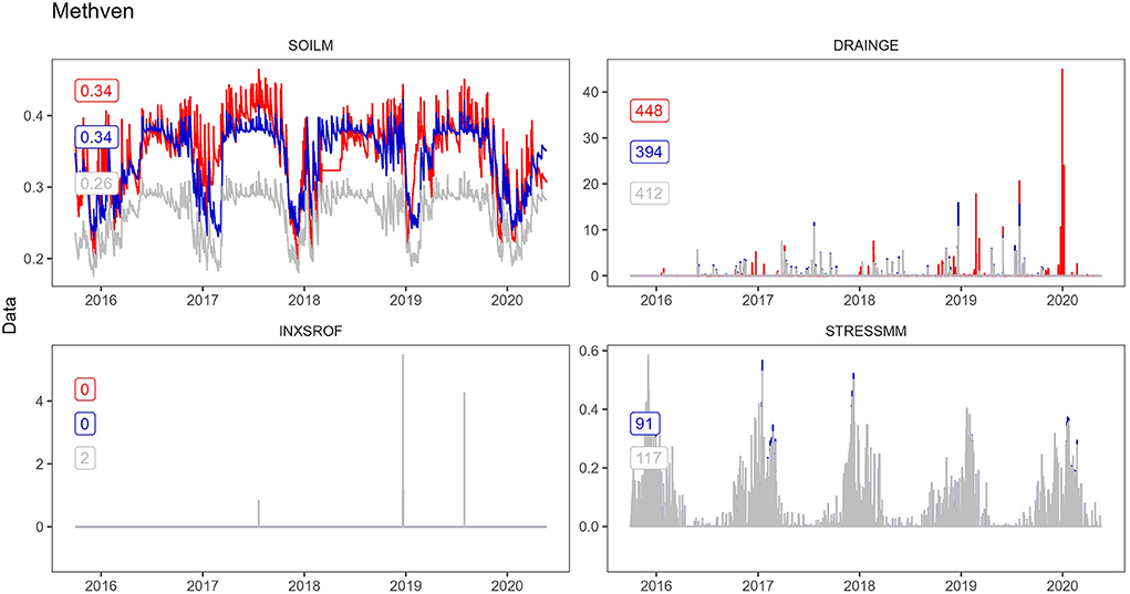
Figure 6. Model output after calibration to Methven data. Red, blue and gray traces indicate the data, calibration and upscaled prediction, respectively. Colored numbers indicate annual averages or totals. Units: SOILM (m3/m3), DRAINGE (m/d), INXSROF (mm/d) and STRESSMM (m3/m3).
Including the change in soil water content as an additional calibration variable allowed the model to reproduce the short-term dynamics of the observed soil water content trace, even though the absolute match to the uncalibrated soil water content sensors was less consistent, perhaps due to a combination of instrument drift, which introduces measurement uncertainty, and model parsimony. Drainage predictions were relatively consistent with the observed data, although the model generally was not able to represent summer drainage (as in a tipping bucket model, drainage can only occur when the soil water content exceeds field capacity, which is rare in summer). Surface runoff was close to zero, as desired (this is assumed to be rare in free draining soils) and water content stress patterns follow climatic conditions with stress periods concentrated in summer.
The calibrated model vs. measured hourly soil water content and drainage for the Methven site are shown in Figure 7, where model values represent the median of the model predictions for 10,000 realizations at each time step. The scatter around this line indicates the model misfit, including any systematic bias. The inclusion of soil water content change as an additional “data” series allowed the modeled soil water content to generally vary in a parallel direction to the 1:1 line. Modeled drainage coincides with rainfall inputs, with only few cases where data and model drainage occurred at different times, a situation which our simple model is unable to reproduce.
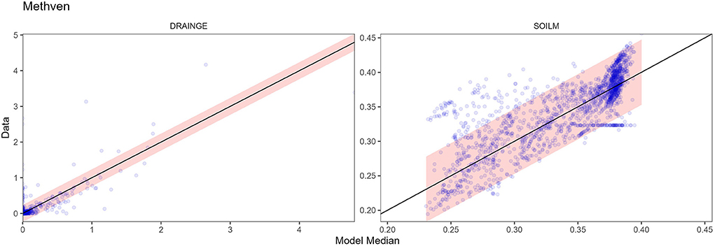
Figure 7. Calibration to Methven soil water content and drainage data. X-axis shows the median of the model predictions for 10,000 realizations at each time step. The shaded area is the 95% region for the residuals. Units: SOILM (m3/m3), DRAINGE (m/d).
Figure 8 shows the marginal posterior parameter distributions for the calibrated model. Parameters with a narrow posterior distribution were able to be determined from the data. Parameters with a wide posterior distribution matching the prior distribution were not able to be determined from the data. Correlations between the parameters can also be checked using a “pairs” plot (see Figure A1). The median parameter values are shown in Figure 8 as vertical lines, whereas the maximum a posteriori (MAP) parameter set is shown as blue dots. Although the MAP parameter set is technically the “best fit”, in practice it is much better to use the entire posterior distribution to represent the model calibration. The MAP parameter set may be somewhat different to the median posterior value, and model predictions based on the MAP parameter set may also not be particularly near the median predicted value. See Figure A2 for an example.
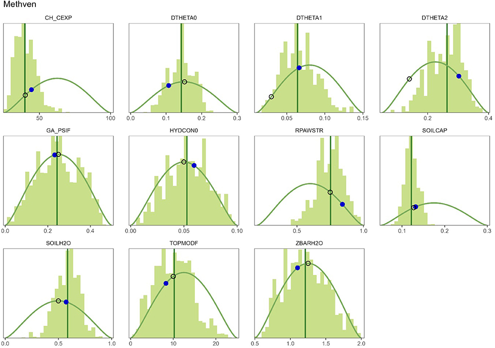
Figure 8. Calibration to Methven data. Parameter (see Table 1) prior distributions (dark green curve), marginal posterior distributions (light green vertical bars), median values (dark green line), maximum a posteriori (MAP) values (blue dot) and upscaled values (black circle). The X-axis units for each subplot are given in Table 1 and the Y-axis is density.
NSE and RMSE are given in Figure 9 for each of the four calibration data series (uncalibrated soil moisture, change in soil moisture, drainage and surface runoff). NSE is not defined for surface runoff (since the daily runoff “data” were all zero); the proportion of days with zero runoff was used instead (PZERO). The perfect fit value (1) is shown as a dotted line on the NSE and PZERO subplots. RMSE results for each data series were compared with the assumed standard errors for the four data series, which were 0.02 (m3/m3), 0.005 (m3/m3/d), 1.0 (mm/d), and 1.0 (mm/d), respectively; these are shown as dotted lines on the RMSE subplots.
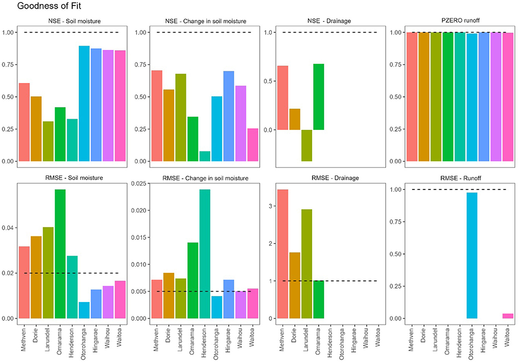
Figure 9. Good of fit across at sites. Nash-Sutcliffe model efficiency (NSE), proportion of zero values (PZERO, for surface runoff only), and root-mean-squared error of predictions (RMSE) for each of the four calibration data series (soil water content, change in soil water content, drainage and surface runoff). Dotted lines show 1 for NSE and PZERO and assumed standard error for RMSE (see Equation 1).
The low NSE for change in soil water content at Henderson reflects the short time period and unusual pattern of the soil water content data at this site (Figure 4). The Henderson soil has a dense clay subsoil (Figure 5), which may result in soil water content patterns that cannot be reproduced with the current model.
The negative NSE for drainage at Larundel may reflect differences in timing between observed and modeled drainage events. Drainage data is difficult to calibrate to, because drainage events are infrequent and flashy. Furthermore, the model can only simulate drainage on the same day that rainfall or irrigation occurs, whereas in reality, drainage may be delayed and/or continue for several days. Even though the RMSE for drainage at this site is not particularly high, the negative NSE indicates that it is higher than the standard deviation of the drainage data. Nevertheless, the pattern of soil water content change and drainage were reasonably simulated at this site, and the average annual drainage was matched reasonably well. This suggests that the negative NSE value is not of concern, and highlights the difficulty of interpreting NSE values in isolation.
Overall, the model fits were reasonable at all sites. The absence of drainage data at the Waikato sites however could result in unrealistic drainage predictions at these sites. This was assessed (below) by comparing the annual predictions across all sites.
The predictive performance of the model calibration across all nine sites was assessed in a simple way by comparing the annual mean or total values of the variables shown in Figure 6 with the field data. The results are shown as filled triangles in Figure 10 (all nine sites had soil water content data, and the four Canterbury sites also had drainage data). As measured soil water content data are uncalibrated, we present plots of calibration vs. measurements (triangles) and calibration vs. upscaled values (circles), rather than data vs. upscaled. However, calibration did a good job of recreating the mean soil water content (SOILM) at each site (although these are uncalibrated sensor measurements). It also did a good job of reproducing the annual drainage (DRAINGE) at the Canterbury sites. The accuracy of the drainage predictions at the Waikato sites is unknown, however. Simulated surface runoff (INXSROF) was also low at all sites, as required.
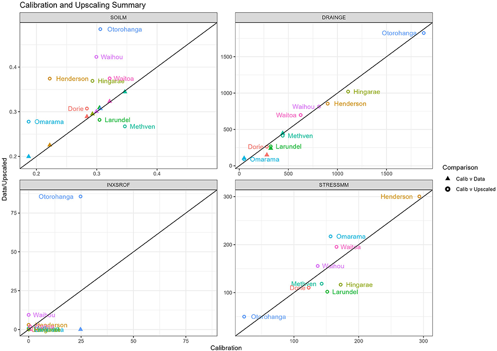
Figure 10. Calibration and upscaling performance. Model annual summaries compared with data [triangles: mean soil water content (SOILM) (m3/m3) at nine sites, and total drainage (DRAINGE) (mm/y) at four sites] and predictions of these variables as well as INXSROF (mm/d) and STRESSMM (m3/m3) based on upscaled parameters (circles).
These results give us confidence that the calibrated parameter distributions at each site (e.g., Figure 8) can be used as the basis for developing an upscaling scheme.
Upscaling of soil hydraulic parameters
The calibrated model parameters were used to develop a simple parameter upscaling scheme to parameterise TopNet (Table 1) for these and other sites (i.e., a transferable method). The posterior parameter distributions for all sites are shown as boxplots in Figure 11. The upscaling scheme is as follows:
• Some parameters were insensitive to the site data, and so could be reasonably set to constant values: HYDCON0 = 0.05 m/s, ZBARH2O = 1.25 m, SOILH2O = 0.5 m, RPAWSTR = 0.75, TOPMODF = 10 m, GA_PSIF = 0.25 m, CH_CEXP = 40, zsoil = 0.75 m (where zsoil = effective soil depth = SOILCAP / (DTHETA1 + DTHETA2).
• The soil water content parameters DTHETA0, DTHETA1 and DTHETA2 were set from the S-map-hydro soil moisture tension points for the near-surface soil layers (see Figure 5 and Section Data preparation). DTHETA0 is not required for model simulations (it is only used for calibration to field data); nevertheless, it was set to the soil water content at −1,500 kPa tension. DTHETA2 was set to the difference between the soil water content at −20 and −1,500 kPa. DTHETA1 was set to the difference between the soil water content at −5 and −20 kPa (this difference yielded the best results). Assuming an effective soil depth (zsoil) of 0.7 m for all sites, this resulted in SOILCAP = zsoil *(DTHETA1 + DTHETA2) values which were similar to the calibrated values across all sites as shown in Figure 11.
• RPAWSTR is the proportion of DTHETA2 below which plant water stress occurs, this was set to a constant value of 0.75 (as all sites are covered by grass).
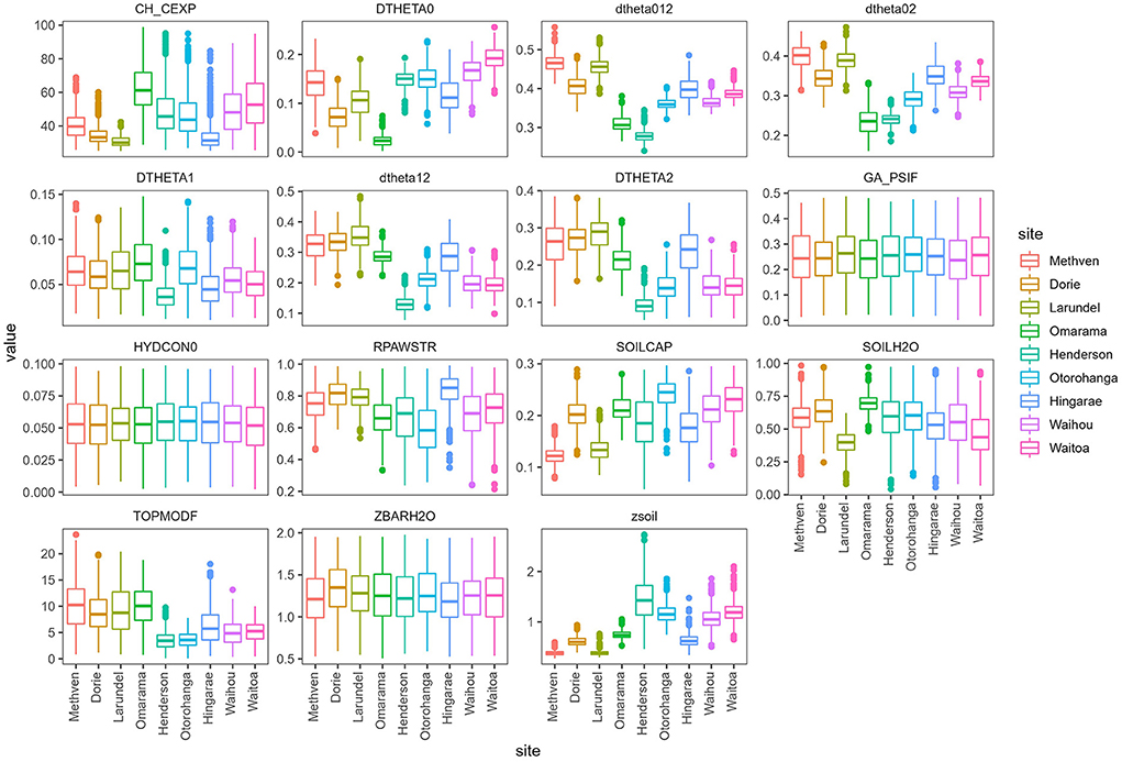
Figure 11. Calibrated and upscaled parameters for all sites. Boxplots show the marginal posterior parameter distributions corresponding to Figure 8. Upscaled parameter values derived from the S-map-hydro soil database (as described in the text) are shown as black dots. The Y-axis units for each subplot are given in Table 1.
The upscaled parameter values are shown as black dots in Figure 11. These parameters were used to generate the gray colored simulations in Figure 6, and shown by black circles in Figure 8.
The overall performance of the parameter upscaling across all nine sites was assessed by comparing the annual mean or total values of the variables shown in Figure 6 with the calibrated prediction and with the field data. The results are shown as open circle in Figure 10, which shows the upscaled mean soil water content (SOILM) was not strongly related to data, as these were uncalibrated. However, as shown in Figure 11 the upscaled soil water parameters (except DTHETA0, which is not required for model simulations) do match the S-map-hydro parameters. Drainage predictions from the model using upscaled parameters closely matched the field data, and the calibrated model at sites where no field data was available. In general, drainage was much higher at the Waikato sites, despite the Canterbury sites being relatively shallower and irrigated. This could be explained by higher Waikato rainfall compared to Canterbury, which average annual rainfall is approximately half that of Waikato. Predicted surface runoff was low at all sites except Otorohanga. Drainage was also high at Otorohanga, while water stress was low; these results reflect the very high rainfall at this site (see Table 4). Water stress (STRESSMM) was relatively low at the irrigated Methven, Doire and Larundel sites, as well as at the Hingarae site. Stress was predicted to be higher at the Waikato's Waihou and Waitoa sites, but Omarama is surprising, since it was irrigated. The very high stress at Henderson may reflect the clay soil at this site, with a low plant water availability, as well as the data period which ran over a very dry summer (2017–2018).
Discussion
This work showed that a simple upscaling technique can be developed to parameterise a single-layer soil water balance module from multilayer (high resolution) data. Previous research (Bresler and Dagan, 1983; Iversen et al., 2001) has illustrated how effective soil water parameters vary with scale. For this reason, we used a calibration scheme to identify the relevant parameters that reflect the system behavior at the scale of interest. Identifying soil parameters using a calibration scheme, however, requires accurate observed data to reduce uncertainty. We used a range of soil water measurements (soil water content); water flux estimates (runoff and drainage); and second order variables (e.g., change in soil water content); to ensure that the calibration scheme resulted in an accurate water balance and associated parameter values. Use of the Bayesian calibration method (Woodward et al., 2020) allowed identification of the most sensitive parameters for soil water content prediction. The Bayesian calibration scheme was used to develop both the “best fit” maximum a posteriori (MAP) parameter set, and a posterior parameter distribution which was utilized for subsequent development of scaling functions. Given the uncertainty of the extent of water flow in the unsaturated zone [primarily due to soil structural heterogeneity and spatial variability (Mallants et al., 1996; Tuli et al., 2001)], use of a posterior distribution allowed incorporation of a range of parameter values rather than using a single parameter set.
The posterior parameter distribution developed for model calibration was used to provide a simple parameter upscaling scheme. Our approach aligned with previous research which have shown that complex small-scale perturbations are reduced at larger scales (Vogel and Roth, 2003; Vogel, 2019). The scaling scheme used to determine “initial” effective parameters for the TopNet model are suitable for simulating multiple soil water properties (e.g., soil water content, drainage and runoff). While the use of observed data is paramount for generating credible soil water parameter values, various configurations of field instruments (soil water content sensors) at the different sites made it difficult to establish a consistent approach across all sites for which measurements were available. For example, soil water content sensors were available for depths up to 1,000 mm at some sites but just 400 mm at other sites. To overcome the challenge posed by various configurations of field instruments, and to develop a consistent approach, only data from near-surface soil water content sensors were used. Again, to be consistent within the upscaling scheme, only S-map-hydro data from near-surface soil layers were used.
It is likely that some of the uncertainty associated with the upscaled parameters is due to the practical limitations imposed by the different configuration of field instruments at each site. While use of the near-surface soil layers does not provide conclusive evidence that the scheme is accurate for the whole profile, we consider that the near-surface dynamics are more important for downward water movement in free draining soils and influence change in soil water behavior in deeper layers within the root zone. However, given the potential uncertainty with the model parametrisation process the upscaled parameters may be treated as “initial representative” parameters, which can be adjusted (preferably within the posterior distribution range described above) during the calibration of the larger hydrological model (i.e., not just the soil water balance submodule). This is also important as field data may not closely match parameters from large scale databases such as S-map-hydro (as shown in Figure 5). Further, as soil heterogeneity exists at all spatial scales and drives most of the parameter uncertainty, the value of soil water properties determined by using measured data at any site should be treated as estimates for other sites, even for soils of the same (soil) series.
Another limitation of the upscaling scheme demonstrated in this study is that the upscaled S-map-hydro parameters cannot be directly used in other hydrological models. For example, the derived parameters would likely need to be altered for use in models with more than one-layer, e.g., the 2-layer LISEM model (De Roo et al., 1996). Our methodology used a Bayesian calibration approach to identify the effective soil water parameters at the scale of interest, and TopNet's soil water balance submodule for calibration. However, the inverse Bayesian calibration and upscaling technique used here can be used for other models using a similar approach.
Other study limitations include: case studies represent only flat grassland, only nine sites were used (i.e., small sample size), soil moisture data used are uncalibrated, drainage data not available at some of the sites, and surface runoff was not measured to close water balance.
The upscaling scheme described in this study develops suitable vertical parameters for the single layer bucket submodule of the TopNet model. However, TopNet is a catchment scale hydrological model. Thus, the suitability of the vertical point-scale soil water parameters at catchment scale needs be further investigated in the future. Further research can also include extending the upscaling framework developed here to other vegetation or land use types, non-free draining soils, soils with contrasting layers down the vertical profile, and use of deeper soil water content data (if available), rather than only from near-surface soil layers.
Conclusion
A Bayesian-based upscaling technique was developed to determine suitable single-layer soil water parameters for a catchment hydrology model, TopNet, based on high resolution S-map-hydro parameters. The technique included two steps: (1) inverse modeling using Bayesian calibration to identify behavioral parameter sets; and (2) an upscaling scheme to estimate suitable soil hydraulic parameters.
In the first step, the single-layer soil-water submodule from TopNet was calibrated using observation data: rainfall, potential evapotranspiration, soil water content, and drainage data. Surface water runoff was assumed to be zero on the free draining soils. The data were also used to develop sets of “best fit” model results and associated posterior parameter distributions. Using the Bayesian calibration process, with 10,000 parameter samples, observed patterns of soil water content change and drainage were able to be simulated reasonably well. However, the model unsurprisingly failed to replicate the exact timing of drainage peaks. This is because the single layer soil module simulates drainage in the same timestep (day) that rainfall or irrigation occurs, even though drainage may actually be delayed or occur over several days. Eleven parameters were considered in the calibration process, however, only eight TopNet parameters were found to be sensitive.
In the second step, a simple parameter upscaling scheme was developed using the posterior distribution of parameters obtained from the calibration procedure described above. Based on S-map-hydro data for the near-surface soil layers, the soil water content parameters of TopNet (DTHETA0, DTHETA1, and DTHETA2) were determined. DTHETA0 represents soil water content at permanent wilting point and was set equal −1,500 kPa (though it was not required for model simulation). Plant available soil water content parameter (DTHETA2) was set to equal the difference between soil water content at tension −20 and −1,500 kPa. DTHETA1, which represents the drainable soil water content, was set to equal the difference between soil water content at tension −5 and −20 kPa. The scaling scheme showed that 0.75 was a suitable value for the relative plant available water at stomatal closure (RPAWSTR) at all nine of the sites modeled.
The upscaling scheme developed in this study demonstrates the effectiveness of combining Bayesian calibration and upscaling to make defensible predictions at ungauged sites. The upscaled model gave realistic predictions of soil water content, drainage, surface runoff, plant water stress patterns and annual totals compared with the field data and the calibrated model. The method could be extrapolated to additional sites where S-map-hydro parameters are available.
Data availability statement
The raw data supporting the conclusions of this article will be made available by the authors, without undue reservation.
Author contributions
CR: conceptualization, method development contribution, data analysis, and manuscript lead. SW: method development, calibration and upscaling, and manuscript contribution. LL and SC: soil-water data analysis and manuscript contribution. JG, MS, CZ, and JF-G: conceptualization, data analysis, and manuscript contribution. All authors have read and agreed to the published version of the manuscript.
Funding
This research was funded by the New Zealand Ministry of Business, Innovation and Employment under the Endeavor program S-map Next Generation (C09X1612).
Acknowledgments
The authors would like to express very great appreciation to Joseph Pollacco, Manaaki Whenua—Landcare Research, Lincoln, New Zealand for developing S-map-hydro data, and his valuable and constructive suggestions during the planning and development of this research. We thank Justin Wyatt, Waikato Regional Council, New Zealand for providing monitored data for the Waikato sites, and Malcolm McLeod, Manaaki Whenua—Landcare Research, Hamilton, New Zealand for providing information about Waikato sites. We also thank Environmental Canterbury, New Zealand for providing access to lysimeter data from Canterbury sites.
Conflict of interest
Authors CR, JG, MS, and CZ are employed by National Institute of Water and Atmospheric Research Limited, Christchurch, New Zealand. Author SW was employed by National Institute of Water and Atmospheric Research Limited, Hamilton, New Zealand. Authors LL and SC are employed by Manaaki Whenua—Landcare Research Limited.
The remaining author declares that the research was conducted in the absence of any commercial or financial relationships that could be construed as a potential conflict of interest.
Publisher's note
All claims expressed in this article are solely those of the authors and do not necessarily represent those of their affiliated organizations, or those of the publisher, the editors and the reviewers. Any product that may be evaluated in this article, or claim that may be made by its manufacturer, is not guaranteed or endorsed by the publisher.
References
Abbaspour, K. C., Van Genuchten, M. T., Schulin, R., and Schläppi, E. (1997). A sequential uncertainty domain inverse procedure for estimating subsurface flow and transport parameters. Water Resour. Res. 33, 1879–1892. doi: 10.1029/97WR01230
Bandaragoda, C., Tarboton, D. G., and Woods, R. (2004). Application of TOPNET in the distributed model intercomparison project. J. Hydrol. 298, 178–201. doi: 10.1016/j.jhydrol.2004.03.038
Beven, K., Lamb, R., Quinn, P., Romanowicz, R., and Freer, J. (1995). “TOPMODEL,” Chapter 18 in Computer Models of Watershed Hydrology, Edited by VP Singh. Highlands Ranch, CO: Water Resources Publications.
Beven, K. J., and Kirkby, M. J. (1979). A physically based, variable contributing area model of basin hydrology/Un modèle à base physique de zone d'appel variable de l'hydrologie du bassin versant. Hydrol. Sci. J. 24, 43–69. doi: 10.1080/02626667909491834
Beven, K. J., Kirkby, M. J., Freer, J. E., and Lamb, R. (2021). A history of topmodel. Hydrol. Earth Syst. Sci. 25, 527–549.
Bresler, E., and Dagan, G. (1983). Unsaturated flow in spatially variable fields: 2. Application of water flow models to various fields. Water Resour. Res. 19, 421–428. doi: 10.1029/WR019i002p00421
Chanasyk, D. S., and Naeth, M. A. (1996). Field measurement of soil moisture using neutron probes. Can. J. Soil Sci. 76, 317–323. doi: 10.4141/cjss96-038
Clark, M. P., Rupp, D. E., Woods, R. A., Zheng, X., Ibbitt, R. P., Slater, A. G., et al. (2008). Hydrological data assimilation with the ensemble Kalman filter: use of streamflow observations to update states in a distributed hydrological model. Adv. Water Resour. 31, 1309–1324. doi: 10.1016/j.advwatres.2008.06.005
Curk, M., and Glavan, M. (2021). “Perspectives of hydrologic modeling in agricultural research,” in Hydrology, eds T. Hromadka II and P. Rao (London: IntechOpen).
De Roo, A. P. J., Wesseling, C. G., and Ritsema, C. J. (1996). LISEM: a single-event physically based hydrological and soil erosion model for drainage basins. I: theory, input and output. Hydrological processes 10, 1107–1117 doi: 10.1002/(SICI)1099-1085(199608)10:8<1107::AID-HYP415>3.0.CO;2-4
Duncan, M. J., Srinivasan, M. S., and McMillan, H. (2016). Field measurement of groundwater recharge under irrigation in Canterbury, New Zealand, using drainage lysimeters. Agric. Water Manag. 166, 17–32. doi: 10.1016/j.agwat.2015.12.002
FAO (2011). The State of the World's Land and Water Resources for Food and Agriculture (SOLAW) – Managing Systems at Risk. Rome and Earthscan, London: Food and Agriculture Organization of the United Nations.
Fernández-Gálvez, J., Pollacco, J. A. P., Lilburne, L., McNeill, S., Carrick, S., Lassabatere, L., et al. (2021). Deriving physical and unique bimodal soil Kosugi hydraulic parameters from inverse modelling. Adv. Water Resour. 153, 103933. doi: 10.1016/j.advwatres.2021.103933
Flury, M., Fluhler, H., Jury, W. A., and Leuenberger, J. (1994). Susceptibility of soils to preferential flow of water - a field-Study. Water Resour. Res. 30, 1945–1954. doi: 10.1029/94WR00871
Gelhar, L. W. (1986). Stochastic subsurface hydrology from theory to applications. Water Resour. Res. 22, 135S−145S. doi: 10.1029/WR022i09Sp0135S
Gelman, A., and Rubin, D. B. (1992). Inference from iterative simulation using multiple sequences. Stat. Sci. 7, 457–472. doi: 10.1214/ss/1177011136
Gómez-Hernández, J. J., and Gorelick, S. M. (1989). Effective groundwater model parameter values: Influence of spatial variability of hydraulic conductivity, leakance, and recharge. Water Resour. Res. 25, 405–419. doi: 10.1029/WR025i003p00405
Graham, S. L., Srinivasan, M. S., Faulkner, N., and Carrick, S. (2018). Soil hydraulic modeling outcomes with four parameterization methods: comparing soil description and inverse estimation approaches. Vadose Zone J. 17, 1–10. doi: 10.2136/vzj2017.01.0002
Green, W. H., and Ampt, G. (1911). Studies on soil physics, 1. The flow of air and water through soils. J. Agric. Sci. 4, 1–24. doi: 10.1017/S0021859600001441
Griffiths, J., Zammit, C., Wilkins, M., Henderson, R., Singh, S., Lorrey, A., et al. (2021). New Zealand Water Accounts Update 2020. NIWA Report 2020325 prepared for Stats NZ Tatauranga Aotearoa, Christchurch.
Hartig, F., Minunno, F., Paul, S., Cameron, D., and Ott, T. (2019). BayesianTools: General-Purpose MCMC and SMC Samplers and Tools for Bayesian Statistics. R Package Version 0.16. Available online at: https://github.com/florianhartig/BayesianTools
Hewitt, A. E. (2010). New Zealand Soil Classification, 3rd Edn. Landcare Research Science Series No.1. Lincoln: Manaaki Whenua Press.
Ibbit, R. (1971). Development of a Conceptual Model of Interception. Unpublished Hydrological Research Progress Report No 5. Ministry of Works, Christchurch, New Zealand.
Iversen, B. V., Moldrup, P., Schjønning, P., and Loll, P. (2001). Air and water permeability in differently textured soils at two measurement scales. Soil Sci. 166, 643–659. doi: 10.1097/00010694-200110000-00001
Jiang, S., Jomaa, S., Büttner, O., Meon, G., and Rode, M. (2015). Multi-site identification of a distributed hydrological nitrogen model using Bayesian uncertainty analysis. J. Hydrol. 529, 940–950. doi: 10.1016/j.jhydrol.2015.09.009
Kosugi, K. (1994). Three-parameter lognormal distribution model for soil water retention. Water Resour. Res. 30, 891–901. doi: 10.1029/93WR02931
Kosugi, K. (1996). Lognormal distribution model for unsaturated soil hydraulic properties. Water Resour. Res. 32, 2697–2703. doi: 10.1029/96WR01776
Lehmann, F., and Ackerer, P. (1997). Determining soil hydraulic properties by inverse method in one-dimensional unsaturated flow. J. Environ. Qual. 26, 76–81. doi: 10.2134/jeq1997.00472425002600010012x
Li, M., Yang, D., Chen, J., and Hubbard, S. S. (2012). Calibration of a distributed flood forecasting model with input uncertainty using a Bayesian framework. Water Resour. Res. 48:20. doi: 10.1029/2010WR010062
Lilburne, L., Webb, T., Palmer, D., McNeill, S., Hewitt, A. S. F., and Fraser, S. (2014). “Pedo-transfer functions from S-map for mapping water holding capacity, soil-water demand, nutrient leaching vulnerability and soil services,” in Nutrient Management for the farm, Catchment and Community, eds L. D. Currie, and C. L. Christensen (Palmerston North: Massey University).
Lilburne, L. R., Hewitt, A. E., and Webb, T. W. (2012). Soil and informatics science combine to develop S-map: a new generation soil information system for New Zealand. Geoderma 170, 232–238. doi: 10.1016/j.geoderma.2011.11.012
Mallants, D., Mohanty, B. P., Jacques, D., and Feyen, J. (1996). Spatial variability of hydraulic properties in a multi-layered soil profile. Soil Sci. 161, 167–181. doi: 10.1097/00010694-199603000-00003
McLeod, M., McGill, A., Thornburrow, D., and Fitzgerald, N. (2015). Soil Data for Waikato Regional Council Soil Moisture Monitoring Network: Sites 6 to 8. Hamilton: Waikato Regional Council by Landcare Research.
McLeod, M., Thornburrow, D., Fitzgerald, N., and Bartlam, S. (2016). Soil Data for Waikato Regional Council Soil Moisture Monitoring Network: Sites 9 and 10. Hamilton: Waikato Regional Council by Landcare Research.
McMillan, H. K., Hreinsson, E. Ö., Clark, M. P., Singh, S. K., Zammit, C., and Uddstrom, M. J. (2013). Operational hydrological data assimilation with the recursive ensemble Kalman filter. Hydrol. Earth Syst. Sci. 17, 21–38. doi: 10.5194/hess-17-21-2013
McNeill, S. J., Lilburne, L., Carrick, S., Webb, T., and Cuthill, T. (2018). Pedotransfer functions for the soil water characteristics of New Zealand soils using S-map information. Geoderma 326, 96–110. doi: 10.1016/j.geoderma.2018.04.011
MfE (2021). Nitrogen Cap Guidance for Regional Councils: Explaining Sections 32–36 of the National Environmental Standards for Freshwater 2020. Wellington: Ministry for the Environment.
MWLR (2022). S-Map - New Zealand's National Digital Soil Map. Lincoln: Manaaki Whenua - Landcare Research.
Nash, J. E., and Sutcliffe, J. V. (1970). River flow forecasting through conceptual models part I—A discussion of principles. J. Hydrol. 10, 282–290. doi: 10.1016/0022-1694(70)90255-6
Pollacco, J. A. P., Fernández-Gálvez, J., Ackerer, P., Belfort, B., Lassabatere, L., Angulo-Jaramillo, R., et al. (2022a). HyPix: 1D physically based hydrological model with novel adaptive time-stepping management and smoothing dynamic criterion for controlling Newton–Raphson step. Environ. Modell. Softw. 153:105386. doi: 10.1016/j.envsoft.2022.105386
Pollacco, J. A. P., Fernandez-Galvez, J., Rajanayaka, C., Zammit, S. C., Ackerer, P., Belfort, B., et al. (2022b). Multistep optimization of HyPix model for flexible vertical scaling of soil hydraulic parameters. Environ. Modell. Softw. 156:105472. doi: 10.1016/j.envsoft.2022.105472
Pollacco, J. A. P., Webb, T., McNeill, S., Hu, W., Carrick, S., Hewitt, A., et al. (2017). Saturated hydraulic conductivity model computed from bimodal water retention curves for a range of New Zealand soils. Hydrol. Earth Syst. Sci. 21, 2725–2737. doi: 10.5194/hess-21-2725-2017
Priestley, C. H. B., and Taylor, R. J. (1972). On the assessment of surface heat flux and evaporation using large-scale parameters. Month Weather Rep. 100, 81–92.
R Core Team (2022). R: A Language and Environment for Statistical Computing. Vienna: R Foundation for Statistical Computing. Available online at: https://www.R-project.org/ (accessed March 25, 2022).
Schoups, G., and Vrugt, J. A. (2010). A formal likelihood function for parameter and predictive inference of hydrologic models with correlated, heteroscedastic, and non-Gaussian errors. Water Resour. Res. 46:17. doi: 10.1029/2009WR008933
Shuttleworth, W. J. (1993). “Evaporation,” in Handbook of Hydrology, ed D. R. Maidment (New York, NY: McGraw-Hill).
Šimunek, J., and Van Genuchten, M.T. (1996). Estimating unsaturated soil hydraulic properties from tension disc infiltrometer data by numerical inversion. Water Resour. Res. 32, 2683–2696. doi: 10.1029/96WR01525
Srinivasan, M.S., Measures, R., and Elley, G. (n.d.). Visualisation of profile available soil water for operational irrigation and drainage management.
Tait, A., Henderson, R., Turner, R., and Zheng, X. (2006). Thin plate smoothing spline interpolation of daily rainfall for New Zealand using a climatological rainfall surface: estimation of daily rainfall over New Zealand. Int. J. Climatol. 26, 2097–2115. doi: 10.1002/joc.1350
Ter Braak, C. J., and Vrugt, J. A. (2008). Differential evolution Markov chain with snooker updater and fewer chains. Stat. Comput. 18, 435–446. doi: 10.1007/s11222-008-9104-9
Tuli, A., Kosugi, K., and Hopmans, J. W. (2001). Simultaneous scaling of soil water retention and unsaturated hydraulic conductivity functions assuming lognormal pore-size distribution. Adv. Water Resour. 24, 677–688. doi: 10.1016/S0309-1708(00)00070-1
Vereecken, H., Kasteel, R., Vanderborght, J., and Harter, T. (2007). Upscaling Hydraulic Properties and Soil Water Flow Processes in Heterogeneous Soils. Vadose Zone J. 6, 1. doi: 10.2136/vzj2006.0055
Vogel, H.-J. (2019). Scale issues in soil hydrology. Vadose Zone J. 18, 1–10. doi: 10.2136/vzj2019.01.0001
Vogel, H.-J., and Roth, K. (2003). Moving through scales of flow and transport in soil. J. Hydrol. 272, 95–106.
Vogeler, I., Carrick, S., Cichota, R., and Lilburne, L. (2019). Estimation of soil subsurface hydraulic conductivity based on inverse modelling and soil morphology. J. Hydrol. 574, 373–382. doi: 10.1016/j.jhydrol.2019.04.002
Vrugt, J. A., ter Braak, C. J. F., Diks, C. G. H., Robinson, B. A., Hyman, J. M., and Higdon, D. (2009). Accelerating markov chain monte carlo simulation by differential evolution with self-adaptive randomized subspace sampling. Int. J. Nonlinear Sci. Numerical Simul. 10, 273–290. doi: 10.1515/IJNSNS.2009.10.3.273
Ward, A. L., Zhang, Z. F., and Gee, G. W. (2006). Upscaling unsaturated hydraulic parameters for flow through heterogeneous anisotropic sediments. Adv. Water Resour. 29, 268–280. doi: 10.1016/j.advwatres.2005.02.013
White, P. A., Hong, Y. S., Murray, D. L., Scott, D. M., and Thorpe, H. R. (2003). Evaluation of regional models of rainfall recharge to groundwater by comparison with lysimeter measurements, Canterbury, New Zealand. J. Hydrol. 42, 39–64.
Woodward, S. J., Van Oijen, M., Griffiths, W. M., Beukes, P. C., and Chapman, D. F. (2020). Identifying causes of low persistence of perennial ryegrass (Lolium perenne) dairy pasture using the Basic Grassland model (BASGRA). Grass Forage Sci. 75, 45–63. doi: 10.1111/gfs.12464
Woodward, S. J. R., Wöhling, T., Rode, M., and Stenger, R. (2017). Predicting nitrate discharge dynamics in mesoscale catchments using the lumped StreamGEM model and Bayesian parameter inference. J. Hydrol. 552, 684–703. doi: 10.1016/j.jhydrol.2017.07.021
Wu, J., and Zeng, X. (2013). Review of the uncertainty analysis of groundwater numerical simulation. Chin. Sci. Bull. 58, 3044–3052. doi: 10.1007/s11434-013-5950-8
Zhang, Z. F., Kachanoski, R. G., Parkin, G. W., and Si, B. (2000a). Measuring hydraulic properties using a line source I. Analytical expressions. Soil Sci. Soc. Am. J. 64, 1554–1562. doi: 10.2136/sssaj2000.6451554x
Zhang, Z. F., Kachanoski, R. G., Parkin, G. W., and Si, B. (2000b). Measuring hydraulic properties using a line source II. Field test. Soil Sci. Soc. Am. J. 64, 1563–1569. doi: 10.2136/sssaj2000.6451563x
Zhang, Z. F., Ward, A. L., and Gee, G. W. (2003). Estimating soil hydraulic parameters of a field drainage experiment using inverse techniques. Vadose Zone J. 2, 201–211. doi: 10.2136/vzj2003.2010
Glossary
Appendix
Appendix A: TopNet point-scale soil water balance model formulation
There are two components of storage of water considered in TopNet as soil column: canopy storage (Sc) and soil or root zone storage (Sr). The movement of water in time t into and out of those storages is described by the following two differential equations:
For each discrete time step Δt, the individual equations above are solved in order from top to bottom, not simultaneously to greatly reduce computation time.
Canopy storage
The time rate of change in canopy storage (Ibbit, 1971) is simulated as:
where p is the precipitation rate above the canopy, pt is the rate of throughfall out of the canopy, and ec is the rate of evaporation from the canopy. Precipitation rate p and the potential evapotranspiration rate are used as model inputs, while throughfall pt and canopy evaporation ec are modeled as a quadratic function of canopy storage.
The rate of through fall, pt is calculated as
where
and Cc is the water holding capacity of the canopy (CANSCAP parameter in Table 1) and f(Sc) represents the fraction of the leaf area that is wet (relative to its maximum).
Canopy evaporation, ec is calculated as
where cr is a parameter (CANENHF parameter in Table 1) used to quantify higher evaporation losses from interception relative to the potential evapotranspiration rate epot, that is computed using the Priestly-Taylor method (Priestley and Taylor, 1972), with radiation terms estimated empirically using the methods in (Shuttleworth, 1993).
Soil storage
The soil or root zone equation is
where i is the infiltration rate, er is the soil evaporation rate and d is the rate of drainage below the root zone to the aquifer.
Infiltration
The infiltration rate i is limited by the canopy throughfall rate pt minus the evaporation rate of the throughfall et, and the maximum infiltration rate i max.
where the evaporation from throughfall is determined by the potential evaporative demand (epot-ec) not met by the canopy evaporation
The maximum infiltration rate, i max, is modeled using a (Green and Ampt, 1911) formulation
where Ψf is the Green-Ampt wetting suction (GA_PSIF parameter in Table 1), zf is the depth of the wetting front and zr is the soil depth. The parameters K0 (HYDCON0 parameter in Table 1) and m (inverse of TOPMODF parameter in Table 1) define the vertical saturated hydraulic conductivity profile of the subsurface (Beven et al., 2021). When zf reaches zr the soil is completely saturated and i max =0. The depth to the wetting front is approximate by
where Sr = θzr, and θ and θsat are the relative soil water contents at actual and saturated condition, respectively.
Soil evaporation
Evaporation from the soil, er, is driven by the potential evaporative demand not met by either the canopy or throughfall evaporation, or epot-(ec+et). It is a function of the relative water content
Where θpa is the plant available relative water content when the available water storage is saturated and is the relative plant available water at stomatal closure (RPAWSTR parameter in Table 1).
Drainage
The drainage rate, d, is a power function of the relative soil water content and is given by
where Kr is the saturated hydraulic conductivity at zr (bottom of the soil layer) and the exponent c (CH_EXP parameter in Table 1) is a function of the unsaturated hydraulic properties of the soil. The value of Kr is calculated as
Appendix B: Additional results
The “pairs” plots that were used to check the correlation between parameters calibrated to soil water content and drainage data, and calibrated TopNet model simulations to the observations for the Methven site are presented below. Similar results along with calibration and upscaling results for other field sites are available for download: https://www.dropbox.com/s/iawctg8o5fl50mk/Supplementary%20Material_Upscaling%20Smap%20hydro.pdf?dl=0.
Figure A1 illustrates the use of a “pairs” plot to check the correlation between parameters calibrated to soil water content and drainage data (for the Methven site). Colinear parameters may appear poorly identified in the marginal posterior plot (Figure 8) but the colinear combination with another parameter may actually be well identified, indicating that two parameters being correlated. On the other hand, non-correlated parameters are also useful, as these can be determined independently.
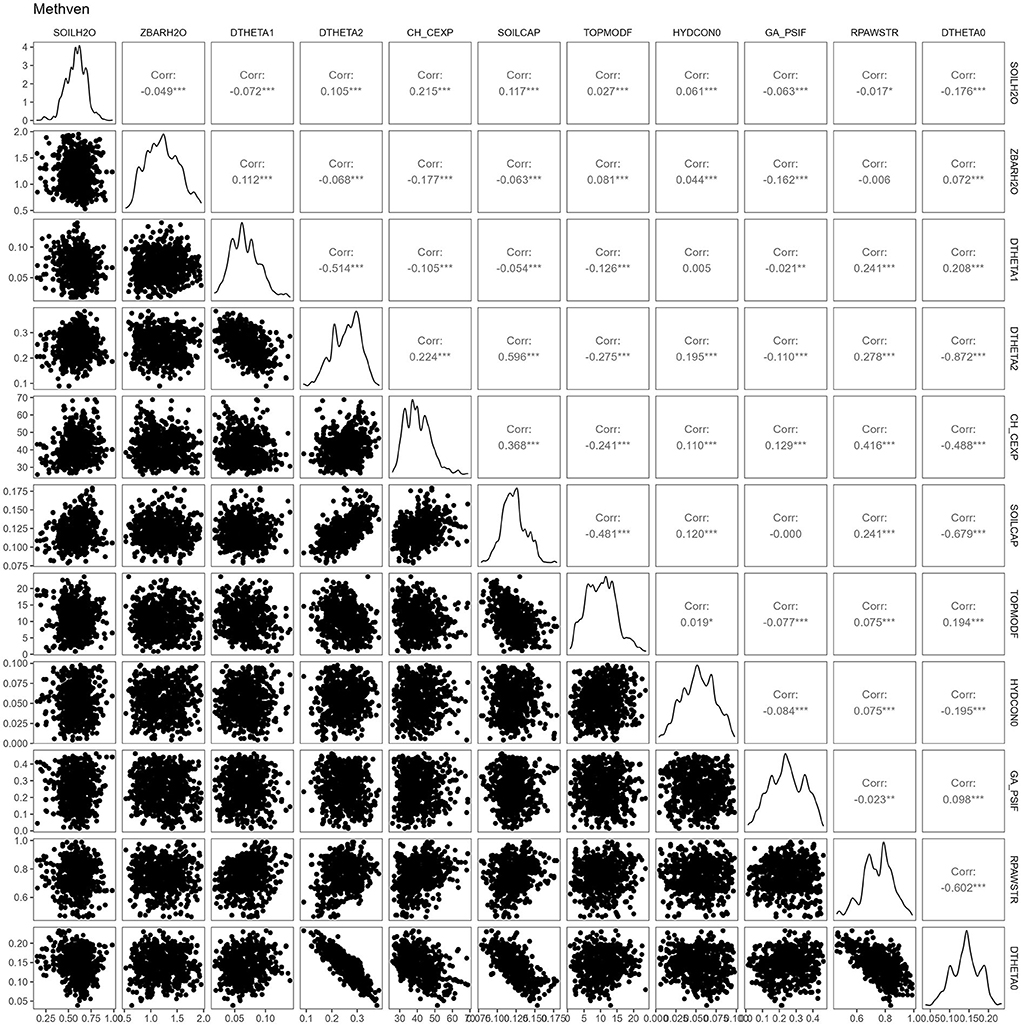
Figure A1. Correlation between parameters calibrated to Methven soil water content and drainage data.
Figure A2 shows the model simulations for the TopNet model calibrated to the Methven data (which are shown in the red DRAINDATA and SOILMDATA traces). Model predictive uncertainty is shown for serval variables, including ZBARH2O, which is the depth to groundwater (mm). ZBARH2O is interesting because it illustrates that the model simulation using the maximum a posteriori (MAP) parameter set (shown in dark blue) may be quite different from the median of the ensemble simulation using all the posterior parameter sets (shown in medium blue). In this case the prediction of ZBARH2O is quite uncertain, but the uncertainty is not symmetrical; the median prediction lies between 1 and 2 metres deep, whereas the MAP prediction is deeper at 1.5 to 2.5 metres deep, as well as having a greater range. This shows that, while reporting the MAP results might appear to be an attractive way to summarise a calibration, these results can be biased in some situations.
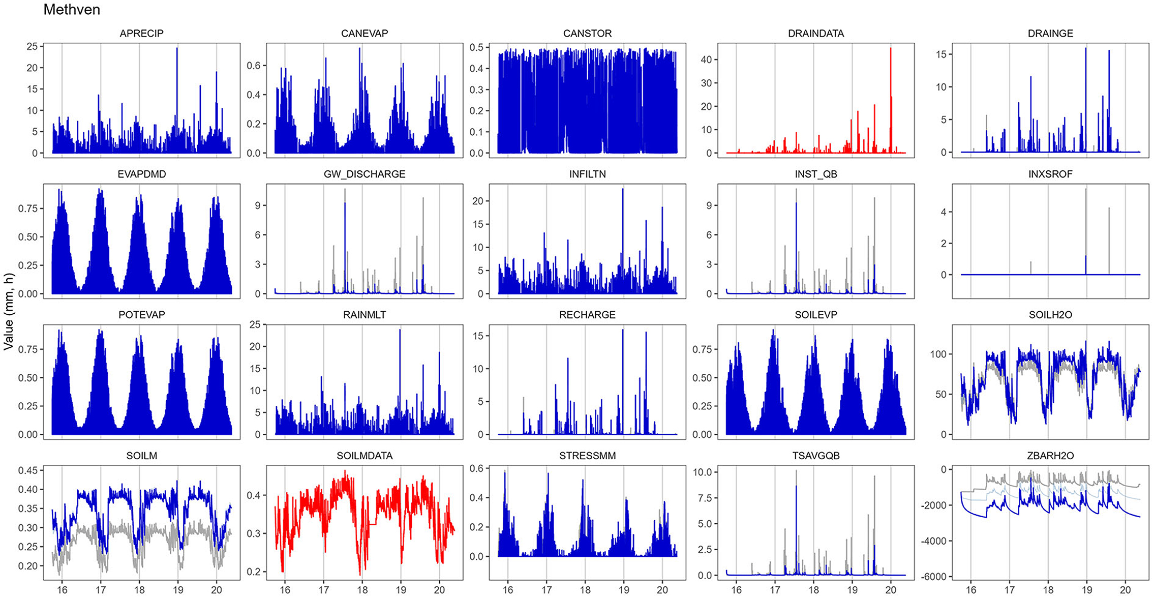
Figure A2. TopNet model simulations calibrated to Methven soil water content and drainage data, with calibration in dark blue, observation data in red, S-map-hydro in grey, and median of the ensemble simulation in medium blue.
Keywords: soil water balance, upscaling of soil hydraulic properties, S-map, New Zealand, 1D hydrological model, parameterization
Citation: Rajanayaka C, Woodward SJR, Lilburne L, Carrick S, Griffiths J, Srinivasan MS, Zammit C and Fernández-Gálvez J (2022) Upscaling point-scale soil hydraulic properties for application in a catchment model using Bayesian calibration: An application in two agricultural regions of New Zealand. Front. Water 4:986496. doi: 10.3389/frwa.2022.986496
Received: 05 July 2022; Accepted: 10 August 2022;
Published: 09 September 2022.
Edited by:
Akhouri Pramod Krishna, Birla Institute of Technology, Mesra, IndiaReviewed by:
Lei Chen, Beijing Normal University, ChinaAnirban Dhar, Indian Institute of Technology Kharagpur, India
Copyright © 2022 Rajanayaka, Woodward, Lilburne, Carrick, Griffiths, Srinivasan, Zammit and Fernández-Gálvez. This is an open-access article distributed under the terms of the Creative Commons Attribution License (CC BY). The use, distribution or reproduction in other forums is permitted, provided the original author(s) and the copyright owner(s) are credited and that the original publication in this journal is cited, in accordance with accepted academic practice. No use, distribution or reproduction is permitted which does not comply with these terms.
*Correspondence: Channa Rajanayaka, Y2hhbm5hLnJhamFuYXlha2FAbml3YS5jby5ueg==
†Present address: Simon J. R. Woodward, DairyNZ, Hamilton, New Zealand