 Alain P. Francés
 Maciek W. Lubczynski
- 1LNEG—Laboratório Nacional de Energia e Geologia, Departamento de Geologia, Hidrogeologia e Geologia Costeira, Lisbon, Portugal
- 2Department of Water Resources (WRS), ITC—Faculty of Geo-Information Science and Earth Observation, University of Twente, Enschede, Netherlands
The new, two-way coupled, distributed and transient MARMITES-MODFLOW (MM-MF) model, coupling land surface and soil zone domains with groundwater, is presented. It implements model-based partitioning and sourcing of subsurface evapotranspiration (ETss) as part of spatio-temporal water balance (WB). The partitioning of ETss involves its separation into evaporation (E) and transpiration (T), while the sourcing of E and T involves separation of each of the two into soil zone (Esoil and Tsoil) and groundwater (Eg and Tg) components. The objective of that development was to understand the system dynamics of a catchment with shallow water table, through spatio-temporal quantification of water fluxes and evaluation of their importance in water balances, focusing on the Eg and Tg components of ETss. While the Eg is computed using formulation from published study, the Tg is obtained through a novel phenomenological function, based on soil moisture availability and transpiration demand driven by climatic conditions. The MM-MF model was applied in the small La Mata catchment (~4.8 km2, Salamanca Province, Spain), characterized by semi-arid climate, granitic bedrock, shallow water table and sparse oak woodland. The main catchment characteristics were obtained using remote sensing, non-invasive hydrogeophysics and classical field data acquisition. The MM-MF model was calibrated in transient, using daily data of five hydrological years, between 1st October 2008 and 30th September 2013. The WB confirmed dependence of groundwater exfiltration on gross recharge. These two water fluxes, together with infiltration and Esoil, constituted the largest subsurface water fluxes. The Eg was higher than the Tg, which is explained by low tree coverage (~7%). Considering seasonal variability, Eg and Tg were larger in dry seasons than in wet season, when solar radiation was the largest and soil moisture the most depleted. A relevant observation with respect to tree transpiration was that during dry seasons, the decline of Tsoil, associated with the decline of soil moisture, was compensated by increase of Tg, despite continuously declining water table. However, in dry seasons, T was far below the atmospheric evaporative demand, indicating that the groundwater uptake by the tree species of this study constituted a survival strategy and not a mechanism for continued plant growth. The presented MM-MF model allowed to analyze catchment water dynamics and water balance in detail, accounting separately for impacts of evaporation and transpiration processes on groundwater resources. With its unique capability of partitioning and sourcing of ETss, the MM-MF model is particularly suitable for mapping groundwater dependent ecosystems, but also for analyzing impacts of climate and land cover changes on groundwater resources.
1. Introduction
Numerical groundwater flow models constitute a powerful tool for groundwater management as they allow to predict aquifers' dynamic responses in relation to climate, land use and abstraction changes (Batelaan et al., 2003). Such models require both a physical representation of aquifer system and appropriate boundary conditions. While aquifer parameters, as saturated hydraulic conductivity and storativity, are spatially dependent and time invariant, groundwater fluxes such as gross recharge (Rg), groundwater evapotranspiration (ETg), groundwater exfiltration (Exfg) and groundwater inflow/outflow can vary in both space and time. Multiplicity of combinations between parameters and fluxes leads to non-uniqueness of model solutions, which limits their reliability and forecasting capability (Moore and Doherty, 2006; Batelaan and de Smedt, 2007; Schilling et al., 2019).
A possible approach to complement the classic model calibration against hydraulic heads and to minimize non-uniqueness of a model solution is to invest in a dense spatial parametrization of the subsurface domains. However, subsurface data are generally scarce, because invasive methods, such as borehole drilling and associated aquifer tests, are expensive and time-consuming. An alternative is to apply hydrogeophysical and remote sensing techniques (Francés and Lubczynski, 2011; Baroncini-Turricchia et al., 2014; Francés et al., 2014, 2015). Hydrogeophysics (HG) provides efficient, non-invasive methods of subsurface data acquisition to complement the invasive methods and identify subsurface rock heterogeneities and potential high water yield zones (Kirsch, 2009). Remote sensing (RS) techniques focus on Earth observation from space. They are used to detect the main hydrological and hydrogeological features such as groundwater expressions at the surface (springs, wetlands etc.), surface water bodies, but also distinct linear features detectable from space, called lineaments. Lineament detection based on analysis of digital terrain model (DTM) allows to identify the main fault zones, while geomorphological classification supports the mapping of pediments (sub-horizontal hard rock erosion front), inselbergs and weathered areas (Meijerink et al., 2007).
Another complementary approach is to constrain groundwater flow models with spatio-temporally variable groundwater fluxes (Jyrkama et al., 2002; Lubczynski and Gurwin, 2005). However, such assessment is complex and uncertain (Kinzelbach et al., 2002; Hendricks et al., 2003; Xu and Beekman, 2003; Lubczynski and Gurwin, 2005; Lubczynski, 2011) because: (i) subsurface water fluxes, due to their inaccessibility, are by far more difficult to quantify than surface water fluxes and consequently the methods of their estimation are highly uncertain; (ii) subsurface water fluxes are controlled by spatio-temporal variability of precipitation (P) and evapotranspiration (ET) but also by surface and subsurface heterogeneity of geology, soil texture, topography, drainage, vegetation, etc.; (iii) groundwater fluxes are generally small and Rg cannot be reliably determined by subtracting ET from P, since unavoidable small errors in the two lead to high inaccuracy of Rg (Lubczynski, 2011); (iv) ETg is generally neglected or underestimated (Lubczynski, 2000, 2009), which results in the overestimation of the net recharge (Rn = Rg − Exfg − ETg) and therefore erroneous model calibration; and (v) standard, standalone groundwater flow models do not take into account interactions with unsaturated zone, so also do not quantify Exfg that can represent important component of groundwater balance, especially in shallow water table environments (Hassan et al., 2014; El-Zehairy et al., 2018; Daoud et al., 2022).
A common practice in using standalone groundwater flow models, such as the well-know MODFLOW (Harbaugh et al., 2000), is to apply arbitrary, simplistic estimates of groundwater fluxes (typically ETg and Rg) as model input. These fluxes were adjusted a-posteriori during model calibration. Such practices have often been leading to large biases in parameter estimation and erroneous groundwater balances (Batelaan and de Smedt, 2007; Lubczynski, 2009, 2011). The relevance of integrating subsurface fluxes, i.e. not only groundwater but also unsaturated zone fluxes, in hydrological models and water balances, has been emphasized by many researchers (Niswonger et al., 2006; Markstrom et al., 2008; Twarakavi et al., 2008; Lubczynski, 2011; Hassan et al., 2014; Langevin et al., 2017) and important advances have been made during the last two decades in the development of powerful, hydrological models (Paniconi and Putti, 2015; Barthel and Banzhaf, 2016; Amanambu et al., 2020; Haque et al., 2021; Refsgaard et al., 2022). Indeed, these distributed, transient models that simulate surface, unsaturated zone and groundwater processes, called coupled models, also known as integrated hydrological models (IHMs), constitute an efficient and realistic way to compute spatio-temporally catchment water balances through partitioning of precipitation into evapotranspiration, runoff, storage and infiltration. Such coupled models also allow the integration of independent state variables from different sources, such as soil moisture and stream discharge, on top of groundwater heads, to constrain the model calibration (Schilling et al., 2019). Moreover, coupled models can implement the separation, here referred as sourcing, of ET into unsaturated zone and groundwater evapotranspiration (respectively ETu and ETg).
It is already well-known and scientifically accepted that in dry conditions, when shallow soil moisture is depleted, the ET can substantially affect not only the surface and unsaturated zones but also the groundwater (Banta, 2000; Lubczynski, 2000, 2009; Maxwell and Condon, 2016). In water limited environments, the ETg may represent important component of water balance (Miller et al., 2010; Lubczynski, 2011; Balugani et al., 2017). Since its first version, MODFLOW incorporates the EVT Package that computes ETg based on a linear relationship depending on depth to water table. Later, Banta (2000) developed the ETS1 Package for MODFLOW-2000 (Harbaugh et al., 2000), which allows to model ETg using a segmented relationship with water table depth. However, as the evapotranspiration represents two physically different processes, i.e. evaporation (E) and transpiration (T), with two different spatial and temporal characteristics (Guan and Wilson, 2009; Lubczynski, 2011; Orellana et al., 2012; Yang, 2015; Maxwell and Condon, 2016), hydrogeological models need to account them separately. Therefore, not only the sourcing but also the partitioning of ET have to be implemented into hydrological models, by considering the following subsurface evapotranspiration (ETss) components: unsaturated zone evaporation (Eu), groundwater evaporation (Eg), unsaturated zone transpiration (Tu) and groundwater transpiration (Tg). Such partitioning and sourcing of ET would be relevant not only to improve the reliability of models and water balances but also to make prediction scenarios of climate and land use changes, as well as to understand the role of vegetation and soil processes in the water cycle (Lubczynski, 2011; Balugani et al., 2017). Some of such studies have already been performed, but most of them either on transpiration or on evaporation and most of them at the plot or local scales (Shah et al., 2007; Pinto et al., 2014; Balugani, 2021). Therefore, there is a need to implement the partitioning and sourcing of ET fluxes in hydrological distributed models. In particular, the importance of Tg in water use strategy by trees in semi-arid to arid environments was emphasized in the literature (Lubczynski and Gurwin, 2005; Naumburg et al., 2005; David et al., 2007, 2013; Gou and Miller, 2014; Barbeta et al., 2015; Osuna et al., 2015; Barbeta and Peñuelas, 2017; Puertes et al., 2019; Miguez-Macho and Fan, 2021). Complex models at the tree scale, taking into consideration the whole groundwater-soil-plant-atmosphere continuum system and its parameterization, were developed to source T (David et al., 2013; Gou and Miller, 2014). However, to our knowledge, there is only one solution to compute Tg in distributed models (Baird and Maddock, 2005), that was developed for the special case of riparian vegetation. It is thus necessary to integrate Tg of facultative phreatophyte vegetation in hydrological models (Gou and Miller, 2014; Puertes et al., 2019; Knighton et al., 2021).
This paper presents a new distributed and transient model, coupling MARMITES land surface and soil zone model with MODFLOW-NWT groundwater flow model (Niswonger et al., 2011), capable to compute a detailed spatio-temporal water balance at the catchment scale. The objective of such development was to understand the system dynamics of a catchment with shallow water table, through spatio-temporal quantification of water fluxes and evaluation of their importance in water balances, focusing on the Eg and Tg components of ETss. The main novelties of the proposed approach are: (i) partitioning of ETss into evaporation and transpiration; and (ii) sourcing of evaporation (Shah et al., 2007) and transpiration (new phenomenological equation) into unsaturated zone and groundwater components. To demonstrate the MARMITES-MODFLOW model capability in simulating complex hydrological systems, the code was applied in the small La Mata catchment (~4.8 km2), located in the Salamanca Province of Spain (Figure 1). That catchment was previously characterized through integration of RS techniques and non-invasive HG (electrical resistivity tomography, frequency domain electromagnetic survey and magnetic resonance soundings) with hydrogeological field data, to define the geometry and the hydrogeological parameters of the local hard rock aquifers (Francés et al., 2014).
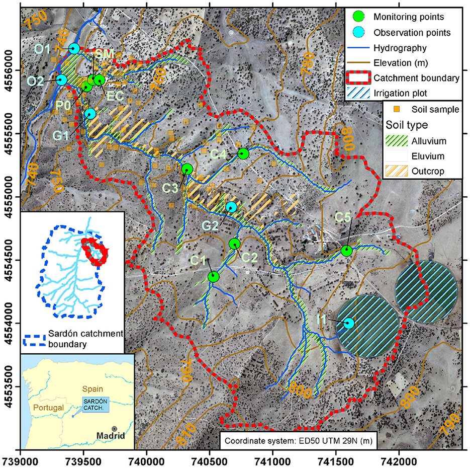
Figure 1. La Mata sub-catchment. Labels indicate monitoring and observation points: G-points in granite outcrops, I-points in irrigation plots and O-points at the outlet.
2. MARMITES-MODFLOW coupled model description
The MARMITES-MODFLOW (MM-MF) model computes water balances at the catchment scale (typically ~10–~1,000 km2) considering storage and flux exchange of water between the following four main hydrological domains (Figure 2, left): land surface, soil zone, percolation zone (unsaturated zone below the bottom of the soil zone and above the water table) and groundwater—in the text below, the index surf refers to the surface, index soil to the soil zone, index p to the percolation zone and the index g to groundwater. Both models, i.e. MM and MF, share the same spatial and temporal discretization. A catchment is divided into squared-grid cells, all of them with the same size (typically from a few meters to several hundred meters). The structure of one cell of the MM-MF is shown in Figure 2 (right). The MM is composed of the surface (MMsurf) and the soil zone (MMsoil) components. The percolation zone is modeled using MODFLOW UZF1 Package (Niswonger et al., 2006), while the groundwater flow is handled by MODFLOW-NWT (Niswonger et al., 2011). The two-way coupling schema (Supplementary Figure 1) allows the boundary flux exchanges between MM and MF. The MM-MF output is a daily, grid-based water balance of a catchment. For each component, the closure of a mass balance is verified using equations shown in Supplementary material (Section 1). More details about the structure and coupling of the MM-MF model are available in Francés (2015).

Figure 2. Conceptual schema of the coupled MARMITES-MODFLOW model, showing the water flux components and the partitioning and sourcing concept. (Left) General scheme describing the exchange of water fluxes between hydrological domains. (Right) Structure of one vertical cell showing the exchange of water fluxes. P, precipitation; EI, interception; Pe, effective precipitation; Eow, open water body evaporation; Ro, surface runoff; Ssurf, land surface storage; I, infiltration; Esoil, soil evaporation; Tsoil, soil transpiration; Ssoil, soil zone storage; n, number of soil layers; Exfg, groundwater exfiltration into soil zone; Rp, percolation from the soil zone; Ep, evaporation from percolation zone; Tp, transpiration from percolation zone; Sp, percolation zone storage; Rg, gross recharge; Eg, groundwater evaporation; Tg, groundwater transpiration; Sg, groundwater storage; Qi/Qo, lateral groundwater inflow/outflow; m, number of aquifer layers. Note that both Ep and Tp are considered negligible and are not computed (indicated with dash lines).
2.1. Surface domain (MARMITES surface)
The main function of MMsurf (Figure 2, right) is to compute the driving forces (effective precipitation, potential evaporation and potential transpiration) on daily basis. Each cell of the MM grid supports only one soil type and one or more plant species individuals (mapped by their canopy areas), contributing to the cell occupancy by their fractional areas (Figure 2, right top). The time discretization is automatically performed by MMsurf based on the precipitation time series analysis.
The surface water balance equation is written as:
where
and
where Ssurf is actual surface water storage, P is precipitation, Pe is effective precipitation, EI is interception by vegetation, Exfg1 is groundwater exfiltration from the topmost soil layer to the surface, I is infiltration into the soil, Eow is evaporation from open water bodies, Ro is surface runoff, ϕ1, θ1 and Dsoil,1 are porosity, actual soil moisture and thickness of the topmost soil layer, respectively. All water fluxes are expressed in [L·T−1] and storage in [L], in mm and in day (also in all the following water balance equations). The land surface in MMsurf is composed of 2 sub-domains (Figure 2, right): the vegetation domain that simulates interception from precipitation and the surface water domain that handles water storage in land depressions and stream channels. When the maximum capacity of the surface water storage is reached, then Ro occurs.
The MMsurf land surface component computes: (i) hourly interception (EI); (ii) daily bare soil potential evaporation (PE); (iii) daily vegetation and agricultural crop potential transpiration (PT); and (iv) daily open water evaporation (Eo). These driving forces are used to compute Pe, Esoil, Tsoil and Eow. The MMsurf requires as input continuous hourly time series of the basic meteorological data, as well as parameters and variables of the meteorological stations, plant species, crops and soil.
The hourly precipitation intensity and duration are used to simulate interception from different plant species, including crops. The storm-based analytical model (Gash, 1979), revised by Gash et al. (1995), was used to estimate interception in sparse forest. This model considers a unit area of canopy to compute wet canopy evaporation, addressed here as rainfall interception (EI). It combines advantages of low data demand with simplicity, still maintaining a realistic approach of the interception process.
A patch model (Yang, 2015) was used to partition the potential evapotranspiration (PET) into potential evaporation (PE) and potential transpiration (PT). In that patch model, the land surface is decomposed into patches with the same plant species or the same soil type. All patches receive the same radiation input but each one is parameterized independently, depending on the soil and plant species, and weighed in each cell of the model as a function of the relative area it occupies. The mapping of plant species and soil patches can be optimally performed using high-resolution (i.e. ~1 m) remote sensing image analysis (Francés and Lubczynski, 2011; Reyes-Acosta and Lubczynski, 2013; Francés et al., 2014), as explained in Section 3.2.
For each soil type, plant species and crop, respective PE and PT are computed using the Penman-Montheith (P-M) equation (Monteith, 1965). In addition to the four meteorological variables (wind speed, air relative humidity, air temperature and incoming solar radiation), the model requires parameters and variables of plant species, crops and soil types (the full lists of parameters are presented in Supplementary Tables 1–3). The definition and values of these parameters and variables of plant species, crops and soil types can be measured in the field (Salinas Revollo, 2010; Balugani et al., 2018). Otherwise, standard values can be found in literature, as for instance in Dingman (2002). To estimate PE, the P-M equation was used with surface resistance of bare soil, computed following van de Griend and Owe (1994). To estimate PT of trees, crops and grass, the P-M equation was also used, defining for each plant species its own set of parameters (Supplementary Tables 1, 2), in particular to compute the canopy resistance (Dingman, 2002). Plant species, crops and soil variables (e.g. albedo, leaf area index) were considered seasonally-constant and a transition period was defined between seasons (Supplementary Tables 1, 2). The model also computes the open water evaporation Eo rate as defined by Penman (Gieske, 2003). Finally, once PT and PE are computed for each plant species, crop and soil type, a weighted averages of PT and of PE are defined at each grid cell, taking into account the fractional area coverage of the plant species, crop and soil type present in that cell.
An irrigation option allows to consider irrigated fields, each one characterized by type of crop, daily irrigation amount and crop schedule (date of seeding and date of cropping). In the cells occupied by crops, the computing of Esoil is seasonally dependent: (i) during the cropping season, it is assumed that the crop coverage is 100% (thus no soil outcropping and Esoil is null); while (ii) when the fields are in fallow, the vegetation coverage, and thus Tsoil, is null and Esoil is computed.
2.2. Soil domain (MARMITES Soil)
The precipitation partitioning and related water balance in the soil zone are computed on daily basis by the MMsoil component using lumped-parameters and linear relationships between fluxes, driving forces and soil moisture.
In each cell of the MM grid, one single soil type is defined. The soil zone is vertically discretized into superimposed layers (Figure 2, right) that are parameterized with basic soil hydraulic properties (Supplementary Table 3). Generally these soil layers are defined using textural criterion and correspond to the A and B horizons, which are the zones of eluviation and illuviation, respectively (Dingman, 2002; Food and Agriculture Organization, 2006). The user can alternatively define one single soil zone corresponding to the root zone.
The water balance in the soil zone is computed as:
where Ssoil is actual soil storage, I is infiltration into the topmost soil layer (downward flux), Exfg is groundwater exfiltration into the bottom soil layer (upward flux), Rp is percolation between soil layers (downward flux), (Exfg)i is groundwater exfiltration from soil layer i to soil layer (i−1) (upward flux), Esoil is bare soil evaporation, Tsoil is vegetation transpiration from soil zone, i is the soil layer index, counted from top to bottom and n is the total number of soil layers.
The Rp of the i-th layer is computed for each layer in the sequence of n-layers using its linear relationship with soil moisture (van der Lee and Gehrels, 1997; Gehrels and Gieske, 2003):
where Ksat is soil saturated hydraulic conductivity, θ is actual soil moisture, ϕ is porosity and is adjusted soil moisture at field capacity.
The linearization of the percolation (Equation 3) is shown in Figure 3, where the linear relationship is compared with the percolation rate measured on a soil sample collected in the study area (Section 3). The error associated with the linearization is affecting mainly the low percolation rates (<50 mm.d−1), which is minimized by adjusting the soil moisture at field capacity parameter (θfc) with during model calibration. Another assumption of Equation (3) is that the capillary forces are negligible as compared to the gravitational forces (van der Lee and Gehrels, 1997; Gehrels and Gieske, 2003), which is similar to the assumption made in the UZF Package (Niswonger et al., 2006). That assumption is acceptable in sandy soils but may not be true in clayey soils, particularly in shallow water table environments.
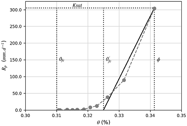
Figure 3. Linear relationship (black straight line) between soil moisture (θ) and soil percolation (Rp, Equation 3). The gray dots represent the experimental percolation rates measured on a soil sample (silty loam) from the study area, first saturated and next exposed to free drainage. ϕ, porosity; θfc, experimental soil moisture at field capacity; , model-adjusted soil moisture at field capacity; Ksat, saturated hydraulic conductivity.
Esoil and Tsoil are obtained using the commonly used linear relationships with soil moisture (van der Lee and Gehrels, 1997; Dingman, 2002) and are computed for each i-th soil layer in the sequence of n-layers as following:
where
and
where
and where θwp is permanent wilting point.
At each time step of MM, Esoil and Tsoil are first taken from the most superficial layer, then from the second soil layer and then further from subsequent layer down to the lowest MMsoil layer. At each soil layer, evaporation and transpiration are subtracted from PE and PT, respectively (Equations 4a and 5a). The sequential computing of Tsoil, from shallow to deepest soil layers, allows to reproduce the observed-pattern of plant water withdrawal (Hillel, 2003; Gou and Miller, 2014; Barbeta et al., 2015). The Equation (4) is applied for bare soil land cover, while the Equation (5) for each plant species, taking into account their fractional area of the grid cells. The computing of Tsoil depends also on the root depth (Zr) defined for each plant species. If the top of a given soil layer is deeper than Zr, i.e. below maximum roots depth, then Tsoil for that layer is null.
2.3. Percolation zone and groundwater (UZF1 and MODFLOW-NWT)
The UZF1 Package (Niswonger et al., 2006) of MODFLOW-NWT (Niswonger et al., 2011), used in the MM-MF coupling framework, simulates the water flow through the percolation zone, i.e. the zone below the soil bottom and above the water table. This zone corresponds to the C and R soil horizons, i.e. parent material and bedrock respectively (Dingman, 2002; Food and Agriculture Organization, 2006). The UZF1 considers only one single uniform layer and converts the percolation from the soil zone (output of MMsoil) into gross groundwater recharge applying a 1D kinematic-wave approximation of the Richards' equation, which considers gravitational forces, but neglects capillary forces (Niswonger et al., 2006). If the water table rises above the bottom of the deepest MM soil layer, groundwater exfiltration (Exfg) from the aquifer into the MMsoil zone occurs, eventually creating saturation-excess overland flow (also known as Dunnian flow) if all the soil layers turn saturated. Finally, groundwater flow and storage are computed by MF.
The water balance in the UZF1 percolation zone is:
where Sp is actual percolation zone storage, Rp is percolation from the soil zone, Rg is gross groundwater recharge and ETp is evapotranspiration from the percolation zone.
The relationships between unsaturated hydraulic conductivity and water content used in UZF1 to simulate the water percolation between the soil zone and the water table are based on the Brooks-Corey equation (Niswonger et al., 2006). That equation requires 4 variables: initial and saturated water contents, saturated hydraulic conductivity and the Brooks-Corey exponent (respectively thti, thts, vks and eps). Despite in UZF1 it is possible to compute ETp, there is no partitioning option. As such, it is not considered in the MM-MF framework and the option to compute ETp is deactivated.
The groundwater balance equation is:
where Sg is groundwater storage, Eg is groundwater evaporation, Tg is groundwater transpiration, Qi and Qo are groundwater inflow and outflow, respectively, Exfg is groundwater exfiltration into the soil zone and m is the total number of MF layers. Eg and Tg are computed by Equations (8) and (9), respectively (see Section 2.4). In this study, the ETg = Eg + Tg is assigned to groundwater extraction (Qw), implemented in MF using the Well Package (see Supplementary Figure 1 and related explanations in the Supplementary material). The other fluxes are computed by the MODFLOW-NWT code.
The groundwater flow equation (Harbaugh, 2005) is numerically solved in MODFLOW-NWT using the finite-difference method and is applied to both confined and unconfined aquifers after correction of the storage term. The time domain is divided into stress periods (SP), during which the water fluxes are constant. When a SP corresponds to several days, the MM water flux rates provided to MF are averaged.
2.4. Partitioning and sourcing of evapotranspiration
After computing Esoil and Tsoil, if PE and PT are not fully satisfied, then Eg and Tg are computed.
In the MM, the bare soil Eg is computed according to Shah et al. (2007) who found a soil-texture dependent, exponential relationships between the Eg and the water table depth (d) [Figure 4 and Equation (8)].
where
where kE is the groundwater evaporation sourcing factor, PEg is the potential groundwater evaporation, d″ is the decoupling depth, y0 is a correction, b is the decay coefficient and D is the evaporation extinction depth. At water table depth lower or equal than d″, PEg is fully satisfied by groundwater, i.e. Eg/PEg = 1. Otherwise the exponential relationship is applied up to the extinction depth D. Equation (8) is applied on bare soil using specific set of parameters d″, b and y0 defined by Shah et al. (2007) for several soil texture classes or locally derived (Table 1).

Figure 4. Groundwater evaporation (Eg) curves (Equation 8) of the main soil texture classes (after Shah et al., 2007). The soil texture class labeled “sandy loam (field)” corresponds to the results of Balugani et al. (2016) obtained from the La Mata catchment. PEg, groundwater potential evaporation; d, water table depth. Refer to Table 1 to consult the corresponding parameters and to Section 2.4 for detailed explanations.
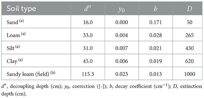
Table 1. Parameters of Equation (8) of: (a) standard soil type (Shah et al., 2007); and (b) La Mata catchment soil type (Balugani et al., 2016).
To quantify the groundwater transpiration (Tg), a novel phenomenological function based on soil moisture availability and transpiration demand, driven by climatic conditions, is proposed. This function was built to reproduce the plant behavior observed during field experiments conducted in the La Mata study area by Reyes-Acosta (2015) and in similar environment in Portugal by David et al. (2013), on three oak tree species (Q.i., Quercus ilex; Q.p., Quercus pyrenaica; Q.p., Quercus suber). These authors quantified the total tree transpiration and contributions from the soil zone and the groundwater. They sampled simultaneously the sap from the tree stems and water of soil layers and groundwater to analyze the stable isotopes content, measuring at the same time the sap flow, the soil moisture and the depth to the water table. Reyes-Acosta (2015) performed the sampling of the tree stem, soil and groundwater once at the end of the wet period (early June 2010) and once at the end of the dry period (September 2009), while measuring sap flow and other variables (long-term monitoring), to study the behavior of Q.i. and Q.p. The soil and groundwater contributions were derived using a model of the whole-tree, constrained by the collected data. David et al. (2013) monitored continuously the hydrological, meteorological, soil and tree variables between March 2007 and December 2008 and sampled the trees stem and roots, soil and groundwater in June and August 2007 and August and September 2008. By analyzing the seasonal sources of sap flow in roots and stem, they were able to model the water uptake and hydraulic redistribution by the shallow, deep and sinker roots and retrieve the monthly contributions of soil and groundwater sources to the tree transpiration.
Using the results of David et al. (2013) and Reyes-Acosta (2015), we computed the soil transpiration sourcing factor kTsoil = Tsoil/T and plotted it against the actual soil moisture (θ) normalized by porosity and wilting point (θnorm) (Figure 5). Next, a sigmoid curve was fitted by adjusting the four plant species sourcing parameters f, s, kTsoilmin and kTsoilmax of the Equation 9. The two parameters f and s define the shape of the sigmoid curve, i.e. f corresponds to the inflection point and s defines the slope. The two other parameters, kTmin and kTmax, set the lower and upper values of kT. These parameters lump together the soil properties and the plant physiology specificities, in particular the hydraulic properties of the conveyance in the plant system (conductance of stem and roots).
where
and where
and where
where f, s, kTmin and kTmax are plant species sourcing parameters, θnorm is normalized soil moisture and PTg is the groundwater potential transpiration.
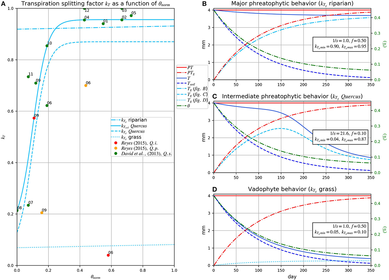
Figure 5. Sourcing transpiration function (Equation 9) and sensitivity analysis of the plant species sourcing parameters: s, f, kTmin and kTmax. (A) kTsoil and kTg as function of normalized soil moisture (θnorm); dots correspond to the observed values of kTsoil of three tree species (Q.i., Quercus ilex; Q.p., Quercus pyrenaica; Q.s., Quercus suber), while labels indicate the month of the measurement. (B–D) Time series of transpiration simulation under constant PT = 3.5 mm.d−1 and declining soil moisture, each with its set of parameters: s, f, kTgmin and kTgmax representing riparian, phreatophytic and vadophytic vegetation; PTg, groundwater potential transpiration; T, total transpiration; Tsoil, soil transpiration; Tg, groundwater transpiration. In the simulations, the following parameters were used: porosity ϕ = 0.45, soil moisture at wilting point θwp = 0.05 and soil thickness = 1.0 m.
As the transpiration mechanism is the same to source Tsoil and Tg, we assumed that the groundwater transpiration sourcing factor kTg shares the same parameter f and s but with lower and upper boundaries defined as:
and
The four plant species sourcing parameters f, s, kTgmin and kTgmax allow to adjust the phreatophytic behavior of plants (further explanations related to applications and interpretation of the Equation 9 can be found in Section 4.2.2). Note that the computing of Tg is also controlled by the root depth (Zr) defined for each plant species, i.e. if the water table depth is deeper than Zr, then Tg is set to zero.
Finally, the subsurface evapotranspiration (ETss) can be computed as:
where
and where
The net groundwater recharge (Rn) can be computed as follows:
3. La Mata catchment study case and model setup
3.1. General description
This study uses the La Mata catchment (~4.8 km2, Figure 1), located west of Salamanca (Spain), to present the functionality of the MM-MF model. The La Mata catchment is a sub-catchment of the Sardón catchment (~80 km2), where extensive research on subsurface water fluxes has been carried out (Lubczynski and Gurwin, 2005; Lubczynski, 2009, 2011; Reyes-Acosta and Lubczynski, 2013; Francés et al., 2014; Hassan et al., 2014; Balugani et al., 2016; Daoud et al., 2022). The La Mata catchment was selected because of a semi-arid, water-limited environment, negligible groundwater use, availability of monitoring data and shallow water table enhancing Eg, Tg and Exfg. The study area is characterized by heterogeneous granitic rock substratum, low to moderate hydraulic conductivity and low storage, typical of hard rock, water scarce condition.
The La Mata catchment has been equipped with an automatic data acquisition system (ADAS, located at P0, Figure 1), which records hourly hydro-meteorological variables since 1996. The water table fluctuation is monitored in one piezometer (~3 m b.g.s.) at the P0 location (automatic, hourly measurement) and at several groundwater-connected ponds (C1–C5, with seasonal observations). Soil moisture was recorded at four depths (0.25, 0.50, 0.75 and 1.00 m) in the alluvium at P0 and in the eluvium at SM (Figure 1). Moreover, an 18 m high eddy covariance (EC) flux tower (Figure 1) was installed at ~140 m NE from the ADAS at P0. That EC tower acquired data between June 2009 and October 2010 allowing to estimate ET (van der Tol, 2012).
The study area, situated at elevation of ~800 m a.s.l., has semi-arid climate, typical for the central part of the Iberian Peninsula. The long-term, 23-years mean precipitation estimated on the base of six Spanish Meteorological Institute rain gauges, located in the surroundings of the study area, is ~500 mm.y−1, while PET ~1,015 mm.y−1. The warmest and the driest months are July and August with an average temperature of ~22°C, average PET of ~5 mm.d−1 and precipitation <20 mm.month−1. The coldest months are January and February with an average temperature of ~5°C and the lowest PET ~0.5 mm.d−1, while the wettest are November and December, with precipitation above 100 mm.month−1 (Lubczynski and Gurwin, 2005). The daily EC tower estimates of actual evapotranspiration ranged from 0.2 mm.d−1 in dry September to 3.5 mm.d−1 in wet April (van der Tol, 2012).
The landscape of the catchment is characterized by a pediment with gentle slopes that corresponds to present and old planation surfaces. It is erratically interrupted by inselbergs, exposed corestones and granite outcrops. A dense drainage network of incised streams, typical for hard rock catchments, is developed along faults. Those are intermittent streams, with water flowing only in wet season and after substantial precipitation events. While the pediment is covered by a thin (0.10–0.75 m) sandy-loam inceptisol (eluvium), alluvial deposits 1–3 m thick, are located along the centrally elongated in approximately N-S direction thalweg (line defining the deepest channel in a valley). The main part of the alluvium profile is composed of silty sand deposited above a 0.5 m thick layer of centimeter to decimeter size pebbles. The shallow subsurface was documented by invasive field methods (portable percussion hammer with sampling gauge, augering and digging). The collected soil samples were analyzed in laboratory to retrieve the hydraulic properties and soil texture.
The land cover is represented by open woodland composed of sparsely distributed evergreen oak Quercus ilex subsp. ballota Desf. (Samp.) and broad-leafed deciduous oak Quercus pyrenaica wild. The canopies of these two oak trees cover ~7% of the La Mata sub-catchment. Their parameters and properties were measured in the field in order to derive PT (Salinas Revollo, 2010; Reyes-Acosta, 2015, see Supplementary Table 1). The entire area is covered by grasses that sprout in March–May, starting to wilt in June and shortly after disappear due to the drying soil and cattle grazing. A shrub species, known as Scotch Broom (Cytisus scoparius), is sparsely distributed in the grass fields.
The water table depth, as monitored in the study area, varies between 0.0 and 3.0 m below ground surface (m b.g.s.) along the thalweg and between 1.0 and 10.0 m b.g.s. at the catchment divides. As the groundwater system is unconfined, the water table follows the topography and is largely influenced by the surficial drainage network. The groundwater pattern is natural due to negligible groundwater abstraction.
3.2. Remote sensing and hydrogeophysics data acquisition
The MM-MF model requires as input spatially distributed parameters that were obtained through field sampling and hydrogeophysical (HG) point and transect measurements that were extrapolated at the catchment scale using remote sensing (RS) techniques (Francés and Lubczynski, 2011; Francés et al., 2014, 2015). The land cover, i.e. soil types, rock outcrops including fracture density, tree species and canopy areas were all identified and mapped using RS techniques at the scale of the Sardón catchment, to which the La Mata sub-catchment belongs. The partitioning of ET at the grid cell scale requires soil and plant species fractional area contributions. The soil types and granite outcrops were mapped as in Francés et al. (2014) using a supervised classification technique applied on two high-resolution, multispectral satellite images: QuickBird from September 2009 (dry season) and WorldView-2 from December 2012 (wet season), to increase the contrast on spectral information between objects. The classification method was based on object-oriented fuzzy-logic analysis (Benz et al., 2004), available in the eCognition software. Two main soil types, i.e. the alluvium and elluvium, were identified and separated from granite outcrops (Figure 1). The mapping of the ground projection of species-dependent tree canopies was made by Reyes-Acosta and Lubczynski (2013), using the same remote sensing technique and the same two images as used for the soil classification. They obtained a map of the canopy areas, including every single tree with 90% probability of being well species-classified. The fractional areas of tree canopies were derived from the mapped canopy covers, following the assumption that tree-root water uptakes affect areas equal to the ground projection of the canopy areas (Naumburg et al., 2005). The areas outside tree canopies, with seasonal grass and patches of Cytisus scoparius (Scotch Broom), including granite outcrops, were lumped together.
Francés et al. (2014) characterized geometrically and parametrically the Sardón catchment using invasive point measurements and non-invasive hydrogeophysical methods such as electrical resistivity tomography, frequency domain electromagnetic survey and magnetic resonance soundings. The results were integrated and distributed at the catchment scale using auxiliary remote sensing data, allowing to define a hydrogeological conceptual model, which identified two main hydrostratigraphic layers, i.e. the saprolite and the fissured layers. That conceptual model was the base of the numerical groundwater flow model of this study.
3.3. Spatial and temporal discretization
The spatial discretization of the La Mata sub-catchment was made on a regular square grid of 50 m resolution, corresponding to 60 columns and 65 rows. The model simulation was carried out during five successive hydrological years, i.e. from 2009 to 2013 (a hydrological year starts from the 1st of October of the previous year and ends on the 30st of September of the specified year), corresponding to 1,949 days converted into 1,240 stress periods (MMsurf aggregated periods of successive 10 days without precipitation). According to the long-term yearly precipitation average (500 mm.y−1), the penultimate simulated hydrological year (2012) was dry (331 mm.y−1) while the last hydrogeological year (2013) was medium-wet (657 mm.y−1), so these two subsequent and contrasting years were selected for graphical presentation of water balances. An initialization “warm-up” period of 4 months (31/05/2008–30/09/2008) was applied to allow the model to reach equilibrium. The first stress period of the “warm up” was run in steady-state conditions, allowing to start the model with average, long-term initial conditions of UZF1 soil moisture and MF hydraulic heads. Input maps of the MM and MF parameters are presented in Supplementary Figures 2–27.
3.4. MM boundary conditions and parametrization
The basic hydro-meteorological variables necessary to obtain the time series of driving forces (P, PE and PT) were acquired from the ADAS station. The soil data obtained by sampling campaigns (Figure 1) and processed in laboratory (Balugani et al., 2016) allowed to retrieve the soil texture and its hydraulic properties (Supplementary Table 3). The lack of sampling at the SE top of the catchment is due to the prohibition of the land-owner to access his area. The alfalfa crop growing in March and cropped in October can be identified in Figure 1 as the two, circle-shape crop fields located in the eastern part of the La Mata sub-catchment. The related irrigation schedule was defined using the program CROPWAT v8.0 (Food and Agriculture Organization, 2009). The initial soil moisture in MMsoil was assigned at porosity minus 0.5%.
3.5. MF boundary conditions and parametrization
The two main hydrogeological layers referred in Section 3.2 (i.e. saprolite and fissured layers) were simulated subdividing each one into three MF sublayers with the same parameterization, but different thicknesses (Supplementary Table 4), to ease model convergence (Barnett et al., 2012). The heterogeneities detected thanks to the geophysical survey (Francés et al., 2014) were respected by implementing the conceptual model into the numerical groundwater flow model. As such, zone-specific parameterization was used for each hydrogeological layer, i.e. along the main fault of Sardón river (talweg), along the secondary faults and in areas without fault. Initial values of parameters, i.e. thickness, hydraulic conductivity, specific yield and specific storage were introduced using values specified in Francés et al. (2014) (see Supplementary Figures 2–27).
The La Mata catchment divide was defined as no-flow boundary, except of the small section near the catchment outlet, which was represented by six cells of MODFLOW Drain Package (DRN) simulating the groundwater outflow of the catchment (points O1 and O2 on DRN cells in Figure 1). The main parameters required by the MF model are listed in Supplementary Table 4. The initial hydraulic heads of the first stress period, ran in steady-state conditions, were assigned at the base of the soil layer.
As Hassan et al. (2014) found that the 18-year (hydrological years 1994–2012) mean value of ETp was only 1.14 mm.y−1, the ETp was not considered in this study. However, in areas with thick unsaturated zone, the ETp may be a significant component of the water balance (Lubczynski, 2009, 2011) and should be considered.
3.6. Parameterization of partitioning and sourcing processes
The sourcing of E was performed using Equations (4) and (8). Both equations were parameterized based on the soil analysis described in Section 3.4. The parameters of the Eg equation (d″, y0, b and D), specific for the La Mata soil texture (Table 1), were computed using the same methodology as in Shah et al. (2007), described by Balugani et al. (2016). First, they acquired field data of soil texture, soil moisture and matric potential in the La Mata catchment. Next, they implemented a HYDRUS-1D simulation based on these data. Eg and Eu (Eu = Esoil + Ep) were separated from the output of HYDRUS-1D model using the SOURCE code of Balugani et al. (2016). The value of Eg was thus obtained as a function of water table depth. Finally, a curve was fitted to this dataset using Equation (8) by varying parameters d″, y0 and b.
The sourcing of T was performed on both tree species, Q.i. and Q.p., using Equation (5) and Equation (9) and the parameters of Table 2 and Figure 5C. The maximum depth of the tree roots was obtained from direct observations along escarpments in the field and from bibliographic references, e.g. Canadell et al. (1996) and David et al. (2004). The grass, Cytisus scoparius and alfalfa crops, which are not considered as phreatophytes, were parameterized to obtain a null to very low Tg, i.e. low values of kTgmin, kTgmax (Table 2) and root depth (Supplementary Tables 1, 2).
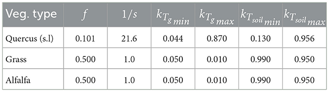
Table 2. Vegetation sourcing parameters (f, s, kTgmin and kTgmax, dimensionless) of Equation (9) defined for the La Mata catchment.
Based on the fractional areas occupied by each tree species and by soil at every grid cell, Esoil, Eg, Tsoil and Tg fluxes were converted into volumes and extracted from the respective domains.
3.7. Calibration
The transient calibration of the MM-MF coupled model was done against: (i) soil moisture in MM at P0 and SM monitoring points; and (ii) hydraulic heads in MF observed at P0. The episodic records of the water level observed in ponds hydraulically linked with groundwater (respectively observation points C1–C5, Figure 1) were also qualitatively used in calibration. The simulated ET was compared with the ET measured by the EC tower. Finally, virtual observation points were inserted in the model to extract water balance and time-series of the hydrological fluxes in different locations with different hydrological conditions (G-points in granite outcrops, I-points in irrigation plots and O-points at the outlet, all identified in Figure 1), which allowed to confirm the coherency of the model solution.
The runoff of the La Mata catchment was estimated on the base of the flume measurement at the Sardón catchment outlet (Ro obs), taking into account the ratio between the two areas, La Mata and Sardón catchments, which is justified due to the same hydrological conditions. Note that the flume-measured Ro obs (up to 145 L.s−1) was sufficient to monitor the baseflow but did not register quick runoff of extreme events.
The calibration process was carried out using trial and error method, aiming to obtain a balanced calibration producing a meaningful water balance and respecting the observation data. The MMsoil component was calibrated by adjusting the soil hydraulic parameters and thickness. The MF model was calibrated adjusting hydraulic conductivity (hk), specific yield (Sy), DRN conductance, UZF1 vertical saturated hydraulic conductivity and UZF1 epsilon factor (vks and eps, respectively).
To analyze the goodness of fit between simulated and observed soil moisture and hydraulic heads, three calibration criteria were used after Moriasi et al. (2007): (i) Pearson's correlation coefficient (r); (ii) root mean square error (RMSE); and (iii) ratio of the RMSE to the standard deviation of the observed heads (RSR). While RMSE and RSR measure the discrepancy between simulated and observed values, r shows how well model and observation trends fit each other. The calibration process focused on minimizing RMSE and RSR and maximizing r.
4. Results and discussion
4.1. MM-MF modeling results
The capability and potential of the MM-MF model are presented through the 5-year (hydrological years 2009–2013) of the real case study simulation of the surface groundwater interactions in the La Mata catchment in Spain. The calibrated time series of soil moisture and hydraulic heads at the monitoring points P0 and SM are presented in Figure 6, while the respective calibration criteria in Supplementary Table 5. The fitting between simulated and observed soil moisture is characterized by r varying between 0.5 and 0.9. RSR and RMSE are also satisfactory, indicating small deviation in relation to observed data. The hydraulic heads at P0 are also well calibrated, respecting the trend and amplitude of the observed data. Its relatively low r = 0.6 and RMSE = 0.9 m can be explained by a temporal shift between simulated and observed data. The calibration also ensured consistent simulated water levels at the catchment outlet (O1 and O2) and at the ponds (C1–C5) in relation to the observed values (Supplementary Figures 28–35). The runoff at the catchment outlet shows expected low calibration indicators due to the limitation of the measurement method, as explained in the Section 3.7, i.e. the flume device was designed to register only low flows, mainly base flow and installed close, but outside the La Mata catchment. The Figure 6 shows a good agreement between the measured low flow and the baseflow derived from the simulated Ro, except in hydrological year 2009, which is close to the “warm-up” period, so influenced by uncertainty of initial conditions. The model simulations of ET time series are also in agreement with the measurements at the EC tower (Figure 6), with r = 0.5 and RMSE = 0.8 mm (Supplementary Table 5). The simulated daily ET varied between 0.1 mm in December 2011 and 2.3 mm in July 2010, which is within a realistic range and shows the same trend as the ET measured by the EC tower (van der Tol, 2012). However, the measured ET amplitude was larger than the simulated, because the tower ET corresponded to the acquisition of almost instantaneous values, while the simulated ET by MM was based on daily simulation.
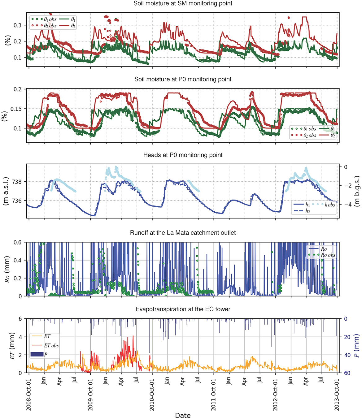
Figure 6. Calibration plots. Locations of SM, P0, La Mata catchment outlet and EC tower as in Figure 1. θn obs, observed soil moisture in the field; θn, simulated soil moisture; n, soil layer index varying between 1 and the total number of soil layers (in this case 2); h obs, observed hydraulic head; hl, simulated hydraulic head; l, MF layer index varying between 1 and the total number of MF layers (in this case 2); m a.s.l., meters above sea level; m b.g.s., meters below ground surface; Ro obs, runoff measured at the Sardón catchment outlet (<145 L.s−1, measured by flume) and corrected using the area ratio (see Section 3.7); Ro, runoff simulated; ET obs, observed evapotranspiration; ET, simulated evapotranspiration; P, precipitation.
The daily time series of simulated surface and subsurface water fluxes, averaged at the catchment scale, are presented in the Figure 7. The 1st plot from the top shows the daily precipitation (P) and the effective precipitation (Pe, Equation 1). As the interception (EI) is low (4% of P) due to the low spatial coverage of trees (~7%) and low storage capacity of alfalfa crops and grass, the Pe differs only a little from the P. The infiltration into soil (I) is important, representing more than 90% of Pe in half of the P events. The surface runoff (Ro) is periodically significant, especially during the last, medium-wet hydrological year 2013. Note that in the current version of the MM-MF model, surface water is not routed to streams, thus the simulated runoff is instantaneous, although in such a small catchment as the La Mata, the routing is not very relevant because the residence time in streams is short, i.e. <1 day. However, for bigger catchments, this MM-MF limitation should be resolved. The 3rd plot shows subsurface evaporation (E) sourced into soil evaporation (Esoil) and groundwater evaporation (Eg) next to potential evaporation (PE). The 4th plot is similar, showing transpiration sourced into soil transpiration (Tsoil), groundwater transpiration (Tg) next to potential transpiration (PT). During the dry seasons neither PE nor PT were reached by E and T, despite the contribution of Eg and Tg, with the lowest difference in the medium-wet hydrological year 2013, when PE and PT were the lowest. The E varied between 0.2 and 2 mm.d−1, reaching its annual maximum just before soil moisture depletion, in April–July (see years 2010 and 2012 in Supplementary Figure 35). The Eg was relatively stable-low during all the years, being almost null in winter and around 0.2 mm.d−1 in dry season, which is much lower than PE. The T contribution to ET was much lower than the E, i.e. similar as in the experimental study by Balugani et al. (2017), showing the maximum of 0.4 mm.d−1 in June 2010 and in June 2012. This is due to the low tree cover in the catchment, which also explains the low value of Tg, which did not reach even 0.1 mm.d−1. The yearly Tg patterns and values were similar throughout the years, except of the last, much wetter year 2013 (annual P was 657 mm), when all transpiration components were substantially lower than in other years because of lower PT. The Tg contribution to T is an important input to reduce water stress in plants, being in this study higher than 50% of T in the peak dry season (typically July–September). However, the T was always lower than the PT, pointing at hydric stress, as reported by David et al. (2004), Gou and Miller (2014). The 5th plot of the Figure 7 presents percolation (Rp), gross recharge (Rg), groundwater exfiltration (Exfg) and groundwater evapotranspiration (ETg). Note that the difference between Rg and Rp is mainly attributed to the storage in the percolation zone, as the ETp is typically, and was indeed, negligible (Equation 6). As expected, the Rg occurred during the wet season, reaching the maxima of 2 mm.d−1 in December 2010 and November 2012. The Rg is only slightly delayed as compared to the Rp, due to shallow water table condition, implying short travel time across the percolation zone. The Exfg is dependent on Rg, resembling its pattern, although with substantially attenuated shape. The Rn (Equation 12) varies between 2 and −0.5 mm, showing positive peaks correlated with P events in wet season. Generally, these peaks are followed by negative values of Rn due to consecutive groundwater exfiltration. In dry season, Rn is negative because of ETg.
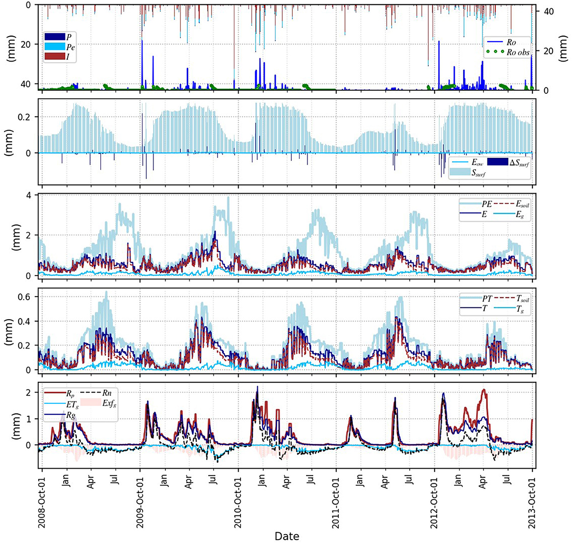
Figure 7. Time series of surface and subsurface water fluxes averaged at the La Mata catchment scale. PE, potential evaporation; PT, potential transpiration. Ro obs, runoff measured at the Sardón catchment outlet and corrected using the area ratio (see Section 3.7). See Figure 2 for other explanations. Soil moisture and hydraulic heads time series are available in Supplementary Figure 35.
The yearly, catchment scale water balance (WB) is presented in Table 3 and illustrated in Figure 8 by Sankey diagrams (Schmidt, 2008), selecting two contrasting hydrological years, the dry year 2012 (P = 331 mm.y−1) and the medium-wet year 2013 (P = 657 mm.y−1). The Esoil, Tsoil, Eg and Tg are higher in 2012 than in 2013, due to larger PE and PT, reflecting climatic conditions with larger solar energy supply. The Esoil and the Exfg represent the highest outfluxes: the Esoil reached 48% of P in 2012 (158 mm) and 23% in 2013 (148 mm), while Exfg was 8% (27 mm) and 15% (102 mm), respectively. The yearly variability of Exfg confirms limited system storage capacity. The Eg is quite stable across 2012 and 2013 (respectively 26 and 20 mm), but its proportion to P is quite different between the 2 years (8 and 3%, respectively), meaning that under shallow water table conditions, such as the one in La Mata catchment, yearly Eg constitutes a relatively constant outflux, independent of the P input. Remarkable is that the Tg reached a value of 9 mm in 2012 against only 2 mm in 2013, which points at its importance for tree survival in dry years. The Rg was much lower in 2012 than in 2013 and Rn was negative in 2012 (−1 mm) but positive in 2013 (18 mm). As a consequence, the superficial aquifer layer, corresponding to the saprolite, shows a loss of storage during the dry year of 2012 (−1 mm) and a subsequent replenishment in 2013 (14 mm). The deeper layer, corresponding to the fractured layer, shows the same behavior, but with very little water flux exchange (Figure 8), which is in agreement with the conceptual hydrogeological model of Francés et al. (2014) that characterized the first layer with higher storage and lower transmissivity and the second layer with lower storage and higher transmissivity.

Table 3. Water balance components in mm per hydrological year (a hydrological year starts from the 1st of October of the previous year and ends on the 30th of September of the specified year).
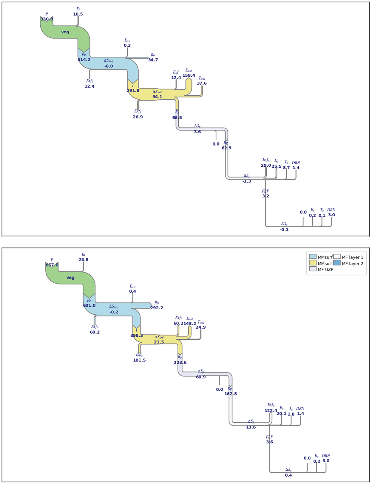
Figure 8. Sankey diagrams representing the yearly water balance at the catchment scale for dry year 2012 (top) and medium-wet year 2013 (bottom). Units in mm.y−1, labels of water fluxes lower than 1E−2 mm.y−1 not shown. Δ—change in storage, DRN—lateral groundwater outflow (Qo) at the catchment outlet simulated using the Drain Package of MODFLOW. See Figure 2 for other explanations.
The spatial variability of water fluxes is visualized in Figures 9, 10 through presentation of selected water fluxes averaged for the five hydrological years of the model simulation. The Esoil is larger than Eg (Figure 9) because in dry season, between July and September, when Esoil is depleted, the Eg, computed following Shah et al. (2007) (Equation 8 and Figure 8), is limited by the depth of the water table, i.e. it is negligible below 5 m. The Esoil is dominant and quite uniformly distributed within the eluvium (Figure 1), while the Eg is high along the stream courses, where the water table is the shallowest (Supplementary Figure 35) and downstream of the agricultural crops due to the irrigation leakage into the groundwater system. The largest Tsoil is observed within the two irrigation plots located at the SE catchment water divide and along the stream courses (Figure 9). The Tg is much lower than the Tsoil, the largest in the southern part of the catchment, where the density of trees is the highest (Supplementary Figure 20). The Figure 10 shows the spatial distribution of the Rg and outfluxes Exfg and ETg, as well as the resultant Rn map, which clearly shows the recharge (Rn > 0, bluish colors) and discharge areas (Rn < 0, reddish colors). The Exfg is related to Ro (Supplementary Figure 36) and concentrated along the streams, showing the dynamic relationship between surface and groundwater in the catchment and the importance of the Dunnian excess overland flow, especially in the medium-wet hydrological year 2013 (Figure 7), when important part of Rg was converted to Exfg.
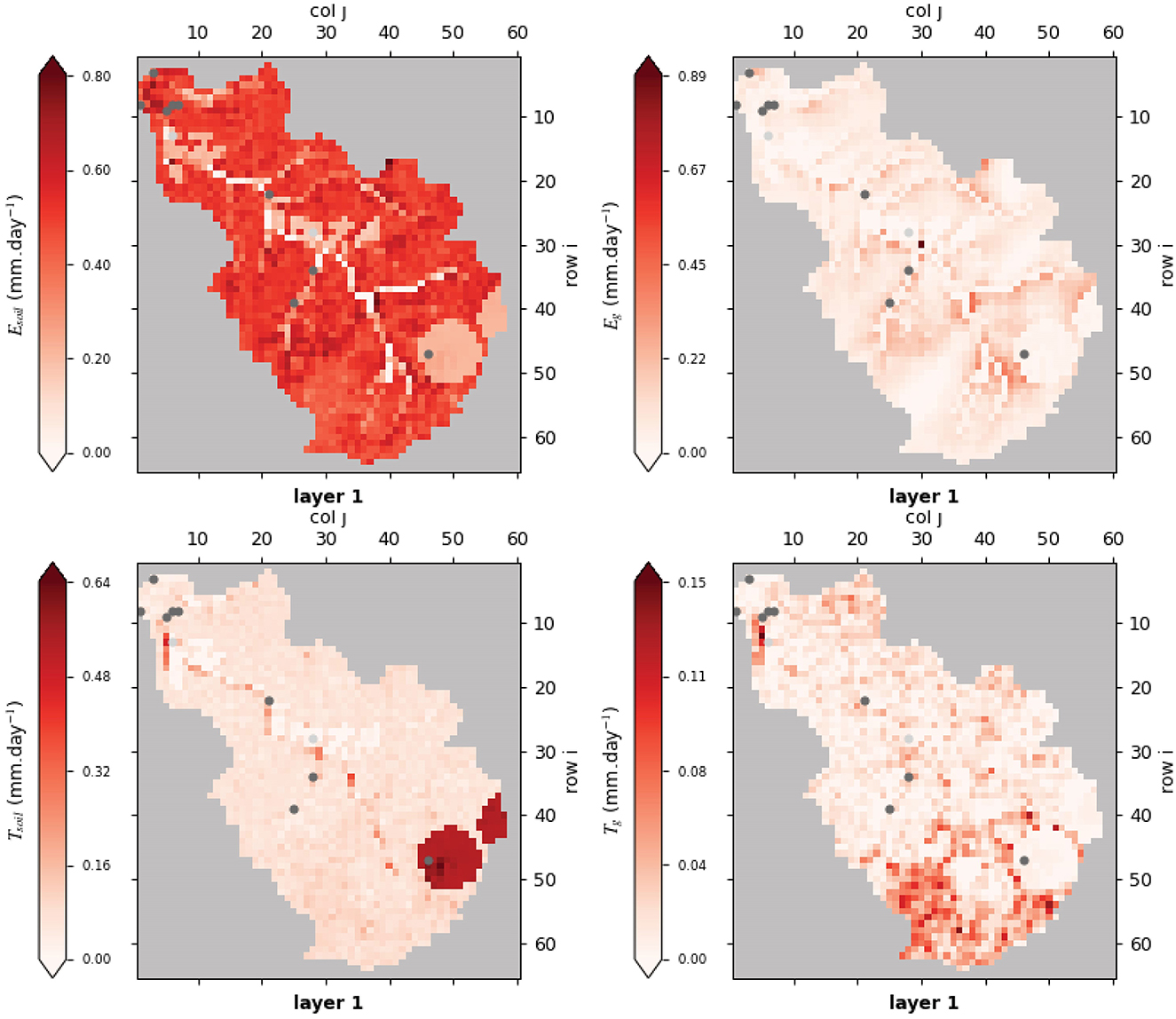
Figure 9. Five-year average of soil evaporation (Esoil, top left), groundwater evaporation (Eg, top right), soil transpiration (Tsoil, bottom left) and groundwater transpiration (Tg, bottom right). Note that each map has its own color scale. The gray dots correspond to the monitoring and observations points of Figure 1.

Figure 10. Five-year average groundwater evapotranspiration (ETg, top left), groundwater exfiltration (Exfg, top right), groundwater gross recharge (Rg, bottom left) and groundwater net recharge (Rn, bottom right). Note that each map has its own color scale. The gray dots correspond to the monitoring and observations points of Figure 1.
4.2. Partitioning and sourcing of evapotranspiration
4.2.1. Groundwater evaporation function
The parameterization of the Equation (8) for the sandy loam soil, based on the soil samples collected in the La Mata catchment and computed by Balugani et al. (2016), is presented in Table 1 and in Figure 4, next to parameters of different soil types presented by Shah et al. (2007). The sandy loam parameters of this study, i.e. d″, y0 and b, are substantially larger than the corresponding parameters defined by Shah et al. (2007). For example, their d″ increases with clay content, being the largest (0.45 m) for the clay, while in this study, the d″ is much larger (1.15 m), even for the sandy loam soil type with lower clay content. The possible reason of that difference could be that Shah et al. (2007) used former version of HYDRUS-1D that considered only liquid water flow (Šimůnek et al., 1998), while Balugani et al. (2016), whom we follow in this study, used the HYDRUS-1D version of Saito et al. (2006), which incorporates heat and vapor transport by diffusion.
The importance of the vapor flow in the dry bare soil conditions has already been emphasized by many researchers (Shokri and Or, 2011; Assouline et al., 2013; Or et al., 2013; Balugani et al., 2016, 2018). However, more recently, Balugani et al. (2021) and Balugani (2021) found that in dry soil layer (DSL) condition, when DSL>5 cm, the vapor diffusion following Saito et al. (2006) plays negligible role. Moreover, Balugani et al. (2023) found that HYDRUS-1D was not able to simulate properly evaporation under DSL> 5 cm, neither in lysimeter nor in-situ, concluding that under DSL> 5 cm dry condition, other than diffusion forces drive vapor flow but those forces are not known, so also not implemented in any numerical flow solution (also not in HYDRUS-1D), yet. Therefore, the sandy loam soil parametrization of bare soil evaporation under very dry soil condition, as it was seasonally the case of this study, could result in substantially different sets of parameters than those provided by Shah et al. (2007).
Experimental estimates of Eg were also carried out by Johnson et al. (2010) and Ma et al. (2019). The former authors used semi-spherical chamber in sand and loam soils, with water table depth varying between 0.1 and 3.3 m, in arid and semi-arid areas of Northern Chile. At shallow depth, they found an exponential relationship relating Eg with water table depth, while at deeper water tables they applied power laws. Their d″ was low, i.e. between 2 and 12 cm, while b varied between 0.036 and 0.072 cm−1. The other authors (Ma et al., 2019) combined in-situ field experiments using a lysimeter with HYDRUS-1D numerical simulations of heat, vapor and liquid water flow in arid Ordos Basin (Inner Mongolia, China) characterized by fine sandy soil. Their d″ was 0.52 m, so higher than the Shah et al. (2007) value of sand (0.16 m) and even higher than the value of clay (0.45 m). In their study, an exponential relation between water table depth and evaporation was observed below d″ and until an extinction depth of 1.05 m.
The differences between parameters of the Equation (8), especially in d″, between the present study, Shah et al. (2007), Johnson et al. (2010) and Ma et al. (2019) suggest that these parameters are site-specific, so should be defined using field data.
4.2.2. Groundwater transpiration function
The four plant species sourcing parameters f, s, kTgmin and kTgmax of Equation (9) allow to adjust the phreatophytic behavior of plants. They were defined using the experimental data set of David et al. (2013) and Reyes-Acosta (2015). Note that the kT values of Reyes-Acosta (2015) in the end of the wet season (June), observable in Figure 5A, are outliers in relation to the other data. Because this author did the experiment with very shallow water table (75 and 125 cm depth) in fine-grained alluvium soil, we assume that there was a bias in the data due to a high capillary fringe and the related mixing of water from soil and groundwater.
The sensitivity analysis, illustrating control of the four plant species sourcing parameters upon the plant behavior in relation to water sources, assuming a constant PT, is presented in Figures 5B–D for three different vegetation behaviors: (i) riparian behavior (Figure 5B): in this case, high values of kTgmin and kTgmax ensure a preponderance of Tg over Tsoil, starting at relatively high soil moisture (~ 20%), while parameters f and s have negligible influence; T almost reaches PT along the whole time series; (ii) phreatophytic behavior (Figure 5C): the beginning of the curves is similar to (i), but as soon as θnorm becomes lower than f, the Tg curve reaches its maximum and start to decrease to stabilize toward a minimum value controlled by kTgmin, but also by f and s; and (iii) minor to null phreatophytic behavior (Figure 5D): low values of kTgmin and kTgmax ensure that Tg is residual and T is dependent on the soil moisture. As such, the use of the four plant species sourcing parameters allows to reproduce the transpiration behavior of plants, including complex behavior of the riparian plants, which keep roots constantly tapping groundwater, but also phreatophytic plants, which can survive droughts by temporal tapping groundwater, such as the oak trees in the La Mata catchment.
The modeling of Tg in the MM-MF framework brought us to the following observations and comments:
(a) Water table depth (d) dependency on Tg: the Figure 5A shows the groundwater transpiration sourcing factor (kTg = Tg/PTg) as function of normalized soil moisture (Equation 9), with groundwater-related constrain that the roots reach the water table. To our knowledge, the only distributed modeling study of sourcing of transpiration is by Baird and Maddock (2005), although they presented quite different transpiration-related approach. They developed a MF package to compute riparian and wetland Tg based on plant physiological characteristics, applying a bell-shaped Tg relation with water table depth (d) that requires plant species specific parameters. As such, that solution was developed for environments with very shallow water table condition, with frequently rising water table above the land surface, creating unfavorable anaerobic conditions leading to a reduction of transpiration and wilting of plants by anoxia. The bell-shaped function, developed for such ecosystems, reflects well their behavior by simulating a Tg decline with water table rise to the surface. However, it is questionable if their solution is applicable to other ecosystems such as the open oak woodland ecosystem of this study or any other, characterized by deeper water table and deeply rooted trees, with access to both soil zone and groundwater. For such settings, it is assumed in this study that if a tree is phreatophytic, i.e. have roots deep enough to be able to tap groundwater, and, if soil moisture is not sufficient to fulfill the tree water demand, then Tg occurs with the rate independent on depth to water table. In fact, there is some impact of declining water table upon Tg as trees require more energy to uplift groundwater. In California savanna with arid climates, Gou and Miller (2014) showed by modeling that, during dry period, both the water table depth (7–12 m b.g.s.) and the plant hydraulic conductance determined the water stress of Quercus douglasii (blue oaks), thus the water table depth might have an influence on the amount of water uptake by trees. However, that dependence was not evident in Barbeta and Peñuelas (2017) (see their Figure 2) as they stated that “the relative contribution of groundwater to transpiration is not affected by the depth of the water table,” although the edaphic conditions (soil vs. fractured bedrock) might have an influence. In our Equation (9), the Tg is dependent on soil moisture depletion, together with climatic demand and maximum depth of roots relative to water table. The effect of a declining water table is not explicit, but indirectly introduced through declining soil moisture. Indeed, at low normalized soil moisture, the kTg factor declines and tends to kTgmin, limiting the amount of groundwater extracted by phreatophytic tree.
(b) Seasonal sourcing of T: the MM-MF model shows that during the wet season, the main contribution to T is from the soil zone, but, during the dry season, Tg contributes with a substantial proportion to T (Figure 7). Indeed, David et al. (2007, 2013), Paço et al. (2009), Miller et al. (2010), Gou and Miller (2014) and Barbeta et al. (2015) independently found that oak trees in savanna environment could compensate low or lack of shallow soil moisture in dry season by taping groundwater at depth of 7–13 m. Barbeta et al. (2015) studied the use of plant-water sources of Q.i and Phillyrea latifolia at the hillslope scale in Mediterranean climate, in hard rock substratum, by inducing long-term (12 years) experimental drought in 150 m2 plots. They found that “the plants extracted water mainly from the soil in the cold and wet seasons but increased their use of groundwater during the summer drought.” Miller et al. (2010) and Gou and Miller (2014) stated that groundwater uptake during dry seasons was thermodynamically favorable over soil water uptake, because “the influence of gravity on water uptake was insignificant compared with the tremendous decline in soil water potential associated with soil drying” (and related increase of rhizosphere and lateral root resistance in the soil layers). David et al. (2004) and David et al. (2007) focused on tree physiology and explained the mechanisms of Tg in oak trees, reproducing the groundwater uptake behavior through modeling at the tree scale (David et al., 2013), which led to an estimate of 30% of stem flow originated from groundwater source on annual basis, which was comparable to the results of Reyes-Acosta (2015), who found that at the end of the dry season (August–September 2009), the Tg of Q.i. varied between 42 and 75% of T during the day, while the Tg of Q.p. between 25 and 35% of T. This confirms that in water limited environments, where trees (e.g. phreatophytes) are adapted to droughts, having deep roots tapping deep soil moisture or groundwater (Lubczynski, 2009), tree transpiration is primarily dependent on climatic forcing and less on shallow soil moisture.
(c) Relatively constant values of T during dry season: the experimental results of Balugani et al. (2017), who partitioned and sourced ET based on field measurements (EC tower, sap flow, soil moisture, groundwater level, isotopes tracing) and HYDRUS modeling, indicate an almost invariant transpiration rate during the late spring throughout the summer period, although the soil moisture was progressively depleted and the water table dropped down more than 1 m (maximum d was 3 m). Throughout that period, the T was stable, because the Tsoil decrease was compensated by the increase of Tg, which took place despite lowering of water table. Gou and Miller (2014) also found that blue oaks were resilient to drought, as during a significantly drier year, the tree transpiration showed just a slight decrease, thanks to substantial increase of the groundwater contribution. This behavior is well reproduced in the MM-MF modeling framework: the transpiration time series (Figure 7) show that for the same order of PT values during the dry season, the T remains almost constant (see also detailed analysis of T time series in previous section).
(d) Tg as a survival strategy: David et al. (2013) and Reyes-Acosta (2015) observed that during the dry period, phreatophytic oak trees do not fully substitute the lack of soil moisture (θ) by groundwater source, i.e. the amount of water needed to fulfill PT is not completely replaced by groundwater. David et al. (2004) monitored oak trees during 2 years in South Portugal and concluded that: “Although there was no increase in water stress during the summer drought, the transpiration rates showed an upper limit well below the atmospheric evaporative demand. This was consistent with the occurrence of a maximum limit for the root water uptake capacity determined by the summer value of whole-plant hydraulic conductance and by stomatal control, which prevented leaf water potential from falling below a cavitation threshold.” Gou and Miller (2014) showed that during droughts, not only the groundwater contribution to T of blue oak was reduced, but also the modeled leaf water potential dropped to low values (−4 to −5 MPa), indicating water stress. As such, groundwater uptake constitutes a tree strategy to mitigate the impacts of drought and not a mechanism for continued plant growth; moreover, groundwater does not constitute a sufficient source of nutrients (Gou and Miller, 2014). As observed in Figure 5A, the ratio kTg = Tg/PTg decreases with decreasing θnorm, which seems counter intuitive, since general understanding is that phreatophytes compensate the shortage of θ by tapping groundwater. However, this way, the Equation (9) allows to limit the amount of extracted groundwater and to compensate the shortage of θ, without fully replacing it, as it was experimentally observed by David et al. (2013), Gou and Miller (2014) and Reyes-Acosta (2015). The results of the MM-MF modeling framework are in agreement with these observations: the transpiration time series (Figure 7) show that besides the Tg contribution to T, also the T is far below the evaporative demand (PT) during the dry period, when the soil moisture is depleted (see Supplementary Figure 35).
(e) Similarity in water use strategy between similar tree species: in our study, we used the same set of parameters of Equation (9) for the two tree species, Q.i. and Q.p., that were mainly derived from measurements made on Q.s. (David et al., 2013). Q.i., Q.p. and Q.s. are assumed to have similar phreatophytic behavior, which may be acceptable at the catchment scale but requires a comparison of water use strategy of different tree species. O'Grady et al. (2009) noted a considerable convergence in plant structure and function, and therefore in water use, among four species of eucalyptus and acacias. Although those species exhibited distinct morphological and physiological patterns, they appeared to operate along what they called a “common physiological continuum.” Knighton et al. (2021) analyzed large dataset of tree species and also found that root water uptake strategies, including groundwater use, are similar among closely related species. David et al. (2007) and Reyes-Acosta (2015) show similarity in trends and water use strategies between the three tree-species of Quercus (Q.i., Q.p. and Q.s.), although the amount of water they extracted varied seasonally. Barbeta et al. (2015), in the same experiment as described above, observed notable differences between Q.i. and Phillyrea latifolia, where Q.i. showed an increase of stem mortality and crown defoliation during extreme drought, together with a decrease of groundwater uptake as compared to previous dry years, indicating a limited access to groundwater, probably due to reduced recharge and deepening of the water table, becoming inaccessible to deep roots. However, these authors observed also that, despite different physiological and morphological characteristics, the Q.i. and Phillyrea latifolia tree species showed similar water use strategy. Therefore, specific characteristics of tree species should be defined experimentally using similar method as proposed by David et al. (2013), Reyes-Acosta (2015), Barbeta et al. (2015), i.e. by performing measurements of sap flow, soil moisture and water table depth, as well as of stable isotopes of all these three media. Recent developments of portable in-situ stable isotopes measurement techniques (Beyer et al., 2020; Mennekes et al., 2021) open an avenue for easier and more reliable than before, in-situ stable isotope data acquisition at high temporal resolution to describe similarities and differences between water use strategies of different plant species; such studies will allow to generalize the parameterization of Equation (9) per groups of similar species. Moreover, the influence of local factors such as topography, geomorphology or edaphic conditions should be also studied to verify their impact on water use strategy of same tree species.
4.3. Comparison with previous studies
In parallel to this study, various other studies were carried out in the same area such as: (i) the ET study, using eddy covariance (EC) tower measurement (van der Tol, 2012); (ii) the tree transpiration studies, first assessing spatial tree transpiration (T) variability by remote sensing upscaling of sap flow measurements (Reyes-Acosta and Lubczynski, 2013), secondary assessing temporal tree transpiration variability by sap flow measurements (Reyes-Acosta and Lubczynski, 2014) and the third sourcing into Tu and Tg using stable isotope experiments (Reyes-Acosta, 2015); (iii) bare soil evaporation (E) study (Balugani et al., 2016, 2018, 2021, 2023; Balugani, 2021), focusing on dry season sourcing of E into Eu and Eg, when grass was dormant, so its T = 0 could be assumed. Moreover, all the three study types were integrated in one, experimental partitioning and sourcing study by Balugani et al. (2017), where Eu, Eg, Tu and Tg were defined separately within the footprint of the EC tower. Their results were compiled in Table 4 and compared with the ET of the EC tower and with the results of the present study. It is remarkable that the partitioning and sourcing of the ET of this study, simulated by MM-MF, was in good agreement with the other corresponding experimental results. The partitioning and the sourcing results of all these studies confirmed the large importance of typically underestimated groundwater evaporation in water balances of savannah type of environments with sparse tree occurrence, such as the La Mata oak woodland study area. Moreover, the consistency between the simulated in this study and the experimental results of Balugani et al. (2017) is an indicator of the good quality of the water flux assessment by the MM-MF modeling.

Table 4. Comparison between the results of: (a) the experimental approach of Balugani et al. (2017); (b) the modeling approach of this study; and (c) eddy tower measurements of evapotranspiration (ET).
Subsurface water fluxes in the Sardón catchment, in which La Mata is a sub-catchment, were modeled by Hassan et al. (2014), who used a GSFLOW model (Markstrom et al., 2008) and also by Daoud et al. (2022), who used MODFLOW 6 (Langevin et al., 2017), both representing transient, distributed solutions. As there is an uniformity of geology, soil, land use and climatic conditions in the two areas, the results of the three models can be compared. For that purpose, we selected the commonly simulated hydrological years 2009–2012 (Figure 11). All the three models show similar results, especially the MM-MF and the one by Daoud et al. (2022), despite different codes and different approaches used. The model of Hassan et al. (2014) provided some differences in water fluxes, mainly because of simplifications in the assignment of driving forces (Daoud et al., 2022), implying higher ETsoil than in the other two models, thus lower Rg and Exfg. Nevertheless, it is remarkable that all these three models, despite using different approaches and parameterization, show consistency. All of them confirm the importance of typically underestimated Exfg in water balances, low catchment storage and low, highly spatio-temporally variable Rn. Although the ETg is about one order of magnitude lower than the ETsoil, it is not negligible, while its Tg component is indispensable for tree survival during droughts, as stated in the Section 4.1 and 4.2.
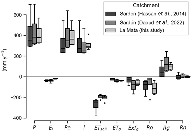
Figure 11. Comparison of the main water fluxes (mm.y−1) of this La Mata study with corresponding water fluxes computed by Hassan et al. (2014) and Daoud et al. (2022) in the Sardón catchment, all presented for the common period of four hydrological years 2009–2012. See Figure 2 for other explanations.
5. Conclusions
This study presents a new, two-way coupled, distributed and transient MM-MF code that implements the partitioning and sourcing of the evapotranspiration fluxes. In particular, a novel phenomenological function was developed to reproduce the behavior of plant transpiration and to quantify the groundwater transpiration (Tg). This function (Equation 9), in contrast to any other available distributed model implementation, is not explicitly dependent on water table depth, but is based on soil moisture availability and transpiration demand, driven by climatic conditions. The parametrization of the Equation 9 requires experimental measurements of sap flow, soil moisture and water table depth as well as of stable isotopes of all these three media. Further studies are required to verify similarities and differences between water use strategies and groundwater uptake by different plant species living in same environment.
The MM-MF code is presented through the model of the La Mata catchment (~4.8 km2), located in water limited environment. The model showed the relevance of Tg during droughts. Indeed, when soil moisture was completely depleted, the Tg allowed to cover important part of plant water demand. The proposed model solution reproduced well the predominant role of climate as driving force of T and the importance of Tg for tree survival during droughts, as pointed by David et al. (2004, 2007), O'Grady et al. (2009), Miller et al. (2010) and Gou and Miller (2014). A relevant issue with respect to transpiration was also that during dry seasons the T/PT ratio was almost constant because the decline of soil moisture and of Tsoil were compensated by increase of Tg occurring simultaneously with decline of water table. This indicates that once trees have roots tapping groundwater, the Tg is then independent (or negligibly dependent) on water table fluctuation. Such trees, known as phreatophytes, can tap interchangeably deep and shallow water resources in order to satisfy the transpiration requirements driven by the climatic conditions. However, in dry seasons, T was far below the atmospheric evaporative demand, indicating that the groundwater uptake by the tree species of this study constituted a survival strategy and not a mechanism for continued plant growth. This behavior was observed in experimental studies carried out in the same area (Reyes-Acosta and Lubczynski, 2014; Balugani et al., 2017) and is also in agreement with other studies performed in other, similar open oak woodland ecosystems (David et al., 2004, 2007, 2013; O'Grady et al., 2009; Paço et al., 2009; Miller et al., 2010; Gou and Miller, 2014).
The groundwater evaporation (Eg) of bare soils was implemented in MM-MF following the methodology proposed by Shah et al. (2007) and Balugani et al. (2016), calibrated with field observations. Our results showed that the Eg was an important component of the water balance (6% of P). However, in other similar studies, local observations must be made a-priori to compute local parameterization for the Equation (8) (Shah et al., 2007). Moreover, the recent research by Balugani et al. (2023) showed that the Eg under dry condition, when DSL>5 cm is developed, can be substantially underestimated.
The MM-MF modeling results of partitioning and sourcing of ET are consistent with corresponding experimental results of Balugani et al. (2017) and with modeling results of Hassan et al. (2014), Daoud et al. (2022), emphasizing the relevance of Exfg in the water balance, as well as generally low, but highly spatio-temporally variable Rn, all representing typical characteristics of hard rock systems with shallow water table such as the La Mata catchment.
The proposed MM-MF modeling framework is applicable not only to hard rocks as in this study but also to other areas, even data scarce. The parametrization of the domains can be facilitated by the use of local measurements extrapolated at the catchment scale using RS and/or HG methods (Francés and Lubczynski, 2011; Francés et al., 2014, 2015). Considering parametrization of temporal variables, the MM-MF may be modified in future to incorporate RS products such as albedo and leaf area index to improve the assessment of driving forces, while ET products can be used as an additional constrain in the model calibration process (Schilling et al., 2019).
The MM-MF model constitutes an effective tool to integrate, at the catchment scale, the fluxes of the surface, soil, percolation zones and groundwater, providing a detailed, spatio-temporal water balance, which includes partitioning and sourcing of ET, to our knowledge not available in any other numerical, distributed, hydrological model. The MM-MF allows also for easy integration of the results of remote sensing and hydrogeophysical data, as well as of the field experimental studies to calibrate or validate model simulation. The specific ability of MM-MF model to partition and source subsurface fluxes constitutes a particularly valuable and novel modeling tool to analyze hydrological and ecohydrological role of tree water uptake and bare soil evaporation, particularly in water limited environments. Such option is expected to be a critical support for land and water management, particularly in assessing the impact of climate and land cover changes on groundwater resources and for mapping groundwater dependent ecosystems.
Data availability statement
The Python source code of the MARMITES model is available at the GitHub code repository under https://github.com/AlainPascalFrances/MARMITES.git/.
Author contributions
AF: fieldwork, data processing, programming, modeling, interpretation, and manuscript writing. ML: fieldwork, conceptualization, supervision and manuscript writing, and proofreading. Both authors contributed to the article and approved the submitted version.
Funding
This study was funded by the Fundação para a Ciência e a Tecnologia through the Programa Operacional Potencial Humano of the QREN Portugal 2007–2013 (Ph.D. scholarship SFRH/BD/27425/2006) and by ITC.
Acknowledgments
The authors would like to thank Jos9 MartFern1ndez (CIALE) for the support in the field logistic as well as the land owners in the Sard3n area, in particular Lucidio Calvo Herrero and Ana Maria Garcia Herrero, for their kind permit to carry out our research within their land property. We acknowledge Enrico Balugani for sharing data and evaporation simulations and the two reviewers, KS and MB, addressing our special thanks to the latter reviewer, for his pertinent comments on plant physiological aspects of groundwater uptake.
Conflict of interest
The authors declare that the research was conducted in the absence of any commercial or financial relationships that could be construed as a potential conflict of interest.
Publisher's note
All claims expressed in this article are solely those of the authors and do not necessarily represent those of their affiliated organizations, or those of the publisher, the editors and the reviewers. Any product that may be evaluated in this article, or claim that may be made by its manufacturer, is not guaranteed or endorsed by the publisher.
Supplementary material
The Supplementary Material for this article can be found online at: https://www.frontiersin.org/articles/10.3389/frwa.2023.1055934/full#supplementary-material
References
Amanambu, A. C., Obarein, O. A., Mossa, J., Li, L., Ayeni, S. S., Balogun, O., et al. (2020). Groundwater system and climate change: present status and future considerations. J. Hydrol. 589:125163. doi: 10.1016/j.jhydrol.2020.125163
Assouline, S., Tyler, S. W., Selker, J. S., Lunati, I., Higgins, C. W., and Parlange, M. B. (2013). Evaporation from a shallow water table: diurnal dynamics of water and heat at the surface of drying sand. Water Resour. Res. 49, 4022–4034. doi: 10.1002/wrcr.20293
Baird, K. J., and Maddock, T. III (2005). Simulating riparian evapotranspiration: a new methodology and application for groundwater models. J. Hydrol. 312, 176–190. doi: 10.1016/j.jhydrol.2005.02.014
Balugani, E. (2021). Partitioning of subsurface evaporation in water limited environments (Ph.D. thesis). Faculty of Geo-Information Science and Earth Observation; University of Twente, Enschede, Netherlands.
Balugani, E., Lubczynski, M., and Metselaar, K. (2016). A framework for sourcing of evaporation between saturated and unsaturated zone in bare soil condition. Hydrol. Sci. J. 61, 1981–1995. doi: 10.1080/02626667.2014.966718
Balugani, E., Lubczynski, M., Reyes-Acosta, L., van der Tol, C., Francés, A., and Metselaar, K. (2017). Groundwater and unsaturated zone evaporation and transpiration in a semi-arid open woodland. J. Hydrol. 547, 54–66. doi: 10.1016/j.jhydrol.2017.01.042
Balugani, E., Lubczynski, M., van der Tol, C., and Metselaar, K. (2018). Testing three approaches to estimate soil evaporation through a dry soil layer in a semi-arid area. J. Hydrol. 567, 405–419. doi: 10.1016/j.jhydrol.2018.10.018
Balugani, E., Lubczynski, M. W., and Metselaar, K. (2021). Evaporation through a dry soil layer: Column experiments. Water Resour. Res. 57:e2020WR028286. doi: 10.1029/2020WR028286
Balugani, E., Lubczynski, M. W., and Metselaar, K. (2023). Lysimeter and in-situ field experiments to study soil evaporation through a dry soil layer under semi-arid climate. Water Resour. Res. 59, e2022WR033878. doi: 10.1029/2022WR033878
Banta, E. (2000). MODFLOW-2000, the U.S. Geological Survey Modular Ground-Water Model—Documentation of Packages for Simulating Evapotranspiration With a Segmented Function (ETS1) and Drains With Return Flow (DRT1). Technical Report 00-466, U.S. Geological Survey.
Barbeta, A., Mejia-Chang, M., Ogaya, R., Voltas, J., Dawson, T. E., and Penuelas, J. (2015). The combined effects of a long-term experimental drought and an extreme drought on the use of plant-water sources in a mediterranean forest. Glob. Change Biol. 21, 1213–1225. doi: 10.1111/gcb.12785
Barbeta, A., and Peñuelas, J. (2017). Relative contribution of groundwater to plant transpiration estimated with stable isotopes. Sci. Rep. 7:10580. doi: 10.1038/s41598-017-09643-x
Barnett, B., Townley, L. R., Post, V., Evans, R. E., Hunt, R. J., Peeters, L., et al. (2012). Australian Groundwater Modelling Guidelines. Waterlines report. Canberra, ACT: National Water Commission.
Baroncini-Turricchia, G., Francés, A. P., Lubczynski, M. W., Martínez-Fernández, J., and Roy, J. (2014). Integrating MRS data with hydrologic model-Carrizal catchment (Spain). Near Surface Geophys. 12, 255–269. doi: 10.3997/1873-0604.2014003
Barthel, R., and Banzhaf, S. (2016). Groundwater and surface water interaction at the regional-Scale—A review with focus on regional integrated models. Water Resour. Manage. 30, 1–32. doi: 10.1007/s11269-015-1163-z
Batelaan, O., and de Smedt, F. (2007). GIS-based recharge estimation by coupling surface-subsurface water balances. J. Hydrol. 337, 337–355. doi: 10.1016/j.jhydrol.2007.02.001
Batelaan, O., De Smedt, F., and Triest, L. (2003). Regional groundwater discharge: phreatophyte mapping, groundwater modelling and impact analysis of land-use change. J. Hydrol. 275, 86–108. doi: 10.1016/S0022-1694(03)00018-0
Benz, U. C., Hofmann, P., Willhauck, G., Lingenfelder, I., and Heynen, M. (2004). Multi-resolution, object-oriented fuzzy analysis of remote sensing data for GIS-ready information. ISPRS J. Photogr. Remote Sens. 58, 239–258.
Beyer, M., Kühnhammer, K., and Dubbert, M. (2020). In situ measurements of soil and plant water isotopes: a review of approaches, practical considerations and a vision for the future. Hydrol. Earth Syst. Sci. 24, 4413–4440. doi: 10.5194/hess-24-4413-2020
Canadell, J., Jackson, R. B., Ehleringer, J. B., Mooney, H. A., Sala, O. E., and Schulze, E.-D. (1996). Maximum rooting depth of vegetation types at the global scale. Oecologia. 108, 583–595. doi: 10.1007/BF00329030
Daoud, M. G., Lubczynski, M. W., Vekerdy, Z., and Frances, A. P. (2022). Application of a novel cascade-routing and reinfiltration concept with a Voronoi unstructured grid in MODFLOW 6, for an assessment of surface-water/groundwater interactions in a hard-rock catchment (Sardon, Spain). Hydrogeol. J. 30, 899–925. doi: 10.1007/s10040-021-02430-z
David, T., Ferreira, M., Cohen, S., Pereira, J., and David, J. (2004). Constraints on transpiration from an evergreen oak tree in southern Portugal. Agric. For. Meteorol. 122, 193–205. doi: 10.1016/j.agrformet.2003.09.014
David, T. S., Henriques, M. O., Kurz-Besson, C., Nunes, J., Valente, F., Vaz, M., et al. (2007). Water-use strategies in two co-occurring Mediterranean evergreen oaks: surviving the summer drought. Tree Physiol. 27, 793–803. doi: 10.1093/treephys/27.6.793
David, T. S., Pinto, C. A., Nadezhdina, N., Kurz-Besson, C., Henriques, M. O., Quilhó, T., et al. (2013). Root functioning, tree water use and hydraulic redistribution in quercus suber trees: a modeling approach based on root sap flow. For. Ecol. Manage. 307, 136–146. doi: 10.1016/j.foreco.2013.07.012
El-Zehairy, A. A., Lubczynski, M. W., and Gurwin, J. (2018). Interactions of artificial lakes with groundwater applying an integrated MODFLOW solution. Hydrogeol. J. 26, 109–132. doi: 10.1007/s10040-017-1641-x
Food and Agriculture Organization (2006). Guidelines for Soil Description. Technical report. Rome: Food and Agriculture Organization of the United Nations.
Food and Agriculture Organization (2009). CROPWAT, A Computer Program for Irrigation Planning and Management. Technical report. Food and Agriculture Organization.
Francés, A. P. (2015). Integration of hydrogeophysics and remote sensing with coupled hydrological models (Ph.D. thesis). ITC-University of Twente, Enschede, Netherlands.
Francés, A. P., and Lubczynski, M. W. (2011). Topsoil thickness prediction at the catchment scale by integration of invasive sampling, surface geophysics, remote sensing and statistical modeling. J. Hydrol. 405, 31–47. doi: 10.1016/j.jhydrol.2011.05.006
Francés, A. P., Lubczynski, M. W., Roy, J., Monteiro Santos, F. A., and Mahmoudzadeh, M. R. (2014). Hydrogeophysics and remote sensing for the design of hydrogeological conceptual models in hard rocks-Sardón catchment (Spain). J. Appl. Geophys. 110, 63–81. doi: 10.1016/j.jappgeo.2014.08.015
Francés, A. P., Ramalho, E. C., Fernandes, J., Groen, M., Hugman, R., Khalil, M. A., et al. (2015). Contributions of hydrogeophysics to the hydrogeological conceptual model of the Albufeira-Ribeira de Quarteira coastal aquifer in Algarve, Portugal. Hydrogeol. J. 23, 1553–1572. doi: 10.1007/s10040-015-1282-x
Gash, J. H. C. (1979). An analytical model of rainfall interception by forests. Q. J. R. Meteorol. Soc. 105, 43–55. doi: 10.1002/qj.49710544304
Gash, J. H. C., Lloyd, C. R., and Lachaud, G. (1995). Estimating sparse forest rainfall interception with an analytical model. J. Hydrol. 170, 79–86. doi: 10.1016/0022-1694(95)02697-N
Gehrels, J. C., and Gieske, A. S. M. (2003). “Aquifer dynamics,” in Understanding Water in a Dry Environment-Hydrological Processes in Arid and Semi-Arid Zones, Vol. 23 of International Contributions to Hydrogeology, ed I. Simmers (Rotterdam: Balkema), 211–250.
Gieske, A. (2003). “Operational solutions of actual evapotranspiration,” in Understanding Water in a Dry Environment : Hydrological Processes in Arid and Semi Arid Zones, Vol. 23, ed I. Simmers (Rotterdam: Balkema), 65–114.
Gou, S., and Miller, G. (2014). A groundwater-soil-plant-atmosphere continuum approach for modelling water stress, uptake, and hydraulic redistribution in phreatophytic vegetation. Ecohydrology 7, 1029–1041. doi: 10.1002/eco.1427
Guan, H., and Wilson, J. L. (2009). A hybrid dual-source model for potential evaporation and transpiration partitioning. J. Hydrol. 377, 405–416. doi: 10.1016/j.jhydrol.2009.08.037
Haque, A., Salama, A., Lo, K., and Wu, P. (2021). Surface and groundwater interactions: a review of coupling strategies in detailed domain models. Hydrology 8:35. doi: 10.3390/hydrology8010035
Harbaugh, A. (2005). MODFLOW-2005, the U.S. Geological Survey Modular Ground-Water Model—The Ground-Water Flow Process. Technical Report 6-A16, U.S. Geological Survey.
Harbaugh, A., Banta, E., Hill, M., and Mc Donald, M. (2000). MODFLOW-2000, the U.S. Geological Survey Modular Ground-Water Model—User Guide to Modularization Concepts and the Ground-Water Flow Process. Technical Report 00-92, U.S. Geological Survey.
Hassan, S. T., Lubczynski, M. W., Niswonger, R. G., and Su, Z. (2014). Surface-groundwater interactions in hard-rocks in Sardón catchment of Western Spain: an integrated modeling approach. J. Hydrol. 517, 390–410. doi: 10.1016/j.jhydrol.2014.05.026
Hendricks, J. M. H., Phillips, F. M., and Harrison, J. B. (2003). “Chapter 5: Water flow processes in arid and semi-arid vadose zones,” in Understanding Water in a Dry Environment - Hydrological Processes in Arid and Semi-Arid Zones, Vol. 23 of International Contributions to Hydrogeology, ed I. E. Simmers (Balkema), 151–210.
Johnson, E., Yáñez, J., Ortiz, C., and Muñoz, J. (2010). Evaporation from shallow groundwater in closed basins in the chilean altiplano. Hydrol. Sci. J. 55, 624–635. doi: 10.1080/02626661003780458
Jyrkama, M., Sykes, J., and Normani, S. (2002). Recharge estimation for transient groundwater modeling. Ground Water 40, 638–648. doi: 10.1111/j.1745-6584.2002.tb02550.x
Kinzelbach, W., Aeschbach, W., Alberich, C., Goni, I., Beyerle, U., Brunner, P., et al. (2002). A Survey of Methods for Groundwater Recharge in Arid and Semi-Arid Regions. Early Warning and Assessment Report Series UNEP/DEWA/RS.02-2. Nairobi: United Nations Environment Programm.
Kirsch, R. (ed.). (2009). Groundwater Geophysics: A Tool For Hydrogeology, 2nd Edn. Berlin: Springer.
Knighton, J., Fricke, E., Evaristo, J., de Boer, H. J., and Wassen, M. J. (2021). Phylogenetic underpinning of groundwater use by trees. Geophys. Res. Lett. 48:e2021GL093858. doi: 10.1029/2021GL093858
Langevin, C. D., Hughes, J. D., Banta, E. R., Niswonger, R. G., Panday, S., and Provost, A. M. (2017). Documentation for the MODFLOW 6 Groundwater Flow Model. U.S. Geological Survey Techniques and Methods 6-A55, U.S. Geological Survey.
Lubczynski, M. (2000). “Groundwater evapotranspiration, underestimated component of the groundwater balance in a semi-arid environment, Serowe case, Botswana,” in Groundwater : Past Achievements and Future Challenges, ed. O. Sililo (Rotterdam: Balkema), 199–204.
Lubczynski, M. (2009). The hydrogeological role of trees in water-limited environments. Hydrogeol. J. 17, 247–259. doi: 10.1007/s10040-008-0357-3
Lubczynski, M. (2011). “Chapter 21: Groundwater evapotranspiration-underestimated role of tree transpiration and bare soil evaporation in groundwater balances of dry lands,” in Climate Change and Its Effects on Water Resources, eds A. Baba, G. Tayfur, O. Gunduz, K. W. Howard, M. J. Friedel, and A. Chambel (Springer), 183–190.
Lubczynski, M., and Gurwin, J. (2005). Integration of various data sources for transient groundwater modeling with spatio-temporally variable fluxes : Sardón study case, Spain. J. Hydrol. 306, 71–96. doi: 10.1016/j.jhydrol.2004.08.038
Ma, Z., Wang, W., Zhang, Z., Brunner, P., Wang, Z., Chen, L., et al. (2019). Assessing bare-soil evaporation from different water-table depths using lysimeters and a numerical model in the Ordos Basin, China. Hydrogeol. J. 27, 2707–2718. doi: 10.1007/s10040-019-02012-0
Markstrom, S., Niswonger, R., Regan, R., Prudic, D., and Barlow, P. (2008). GSFLOW-Coupled Ground-Water and Surface-Water Flow Model Based on the Integration of the Precipitation-Runoff Modeling System (PRMS) and the Modular Ground-Water Flow Model (MODFLOW-2005). U.S. Geological Survey Techniques and Methods 6-D1, U.S. Geological Survey.
Maxwell, R. M., and Condon, L. E. (2016). Connections between groundwater flow and transpiration partitioning. Science 353, 377–380. doi: 10.1126/science.aaf7891
Meijerink, A., Bannert, D., Batelaan, O., Lubczynski, M., and Pointet, T. (2007). Remote Sensing Applications to Groundwater, Vol. 16 of IHP-VI Series on Groundwater. Paris: United Nations Educational Scientific and Cultural Organization (UNESCO).
Mennekes, D., Rinderer, M., Seeger, S., and Orlowski, N. (2021). Ecohydrological travel times derived from in situ stable water isotope measurements in trees during a semi-controlled pot experiment. Hydrol. Earth Syst. Sci. 25, 4513–4530. doi: 10.5194/hess-25-4513-2021
Miguez-Macho, G., and Fan, Y. (2021). Spatiotemporal origin of soil water taken up by vegetation. Nature 598, 624–628. doi: 10.1038/s41586-021-03958-6
Miller, G. R., Chen, X., Rubin, Y., Ma, S., and Baldocchi, D. D. (2010). Groundwater uptake by woody vegetation in a semiarid oak savanna. Water Resour. Res. 46, W10503. doi: 10.1029/2009WR008902
Moore, C., and Doherty, J. (2006). The cost of uniqueness in groundwater model calibration. Adv. Water Resour. 29, 605–623. doi: 10.1016/j.advwatres.2005.07.003
Moriasi, D., Arnold, J., van Liew, M., Bingner, R., Harmel, R., and Veith, L. V. (2007). Model evaluation guidelines for systematic quantification of accuracy in watershed simulations. Trans. ASABE 50:15. doi: 10.13031/2013.23153
Naumburg, E., Mata-gonzalez, R., Hunter, R., Mclendon, T., and Martin, D. (2005). Phreatophytic vegetation and groundwater fluctuations: a review of current research and application of ecosystem response modeling with an emphasis on great basin vegetation. Environ. Manage. 35, 726–740. doi: 10.1007/s00267-004-0194-7
Niswonger, R., Panday, S., and Ibaraki, M. (2011). MODFLOW-NWT, a Newton Formulation for MODFLOW-2005. U.S. Geological Survey Techniques and Methods 6-A37, U.S. Geological Survey.
Niswonger, R., Prudic, D., and Regan, R. (2006). Documentation of the Unsaturated-Zone Flow (UZF1) Package for Modeling Unsaturated Flow Between the Land Surface and the Water Table with MODFLOW-2005. U.S. Geological Survey Techniques and Methods 6-A19, U.S. Geological Survey.
O'Grady, A. P., Cook, P. G., Eamus, D., Duguid, A., Wischusen, J. D. H., Fass, T., et al. (2009). Convergence of tree water use within an arid-zone woodland. Oecologia 160, 643–655. doi: 10.1007/s00442-009-1332-y
Or, D., Lehmann, P., Shahraeeni, E., and Shokri, N. (2013). Advances in soil evaporation physics–a review. Vadose Zone J. 12:vzj2012.0163. doi: 10.2136/vzj2012.0163
Orellana, F., Verma, P., Loheide, S. P., and Daly, E. (2012). Monitoring and modeling water-vegetation interactions in groundwater-dependent ecosystems. Rev. Geophys. 50:RG3003. doi: 10.1029/2011RG000383
Osuna, J. L., Baldocchi, D. D., Kobayashi, H., and Dawson, T. E. (2015). Seasonal trends in photosynthesis and electron transport during the mediterranean summer drought in leaves of deciduous oaks. Tree physiol. 35, 485–500. doi: 10.1093/treephys/tpv023
Paço, T. A., David, T. S., Henriques, M. O., Pereira, J. S., Valente, F., Banza, J., et al. (2009). Evapotranspiration from a mediterranean evergreen oak savannah: the role of trees and pasture. J. Hydrol. 369, 98–106. doi: 10.1016/j.jhydrol.2009.02.011
Paniconi, C., and Putti, M. (2015). Physically based modeling in catchment hydrology at 50: Survey and outlook. Water Resour. Res. 51, 7090–7129. doi: 10.1002/2015WR017780
Pinto, C. A., Nadezhdina, N., David, J. S., Kurz-Besson, C., Caldeira, M. C., Henriques, M. O., et al. (2014). Transpiration in quercus suber trees under shallow water table conditions: the role of soil and groundwater. Hydrol. Process. 28, 6067–6079. doi: 10.1002/hyp.10097
Puertes, C., Lidón, A., Echeverría, C., Bautista, I., González-Sanchis, M., del Campo, A. D., et al. (2019). Explaining the hydrological behaviour of facultative phreatophytes using a multi-variable and multi-objective modelling approach. J. Hydrol. 575, 395–407. doi: 10.1016/j.jhydrol.2019.05.041
Refsgaard, J. C., Stisen, S., and Koch, J. (2022). Hydrological process knowledge in catchment modelling – lessons and perspectives from 60 years development. Hydrol. Process. 36:e14463. doi: 10.1002/hyp.14463
Reyes-Acosta, J. (2015). Tree-water interactions at varying spatio-temporal scales in water limited environments (Ph.D. thesis). ITC-University of Twente, Enschede, Netherlands.
Reyes-Acosta, J., and Lubczynski, M. (2014). Optimization of dry-season sap flow measurements in an oak semi-arid open woodland in Spain. Ecohydrology 7, 258–277. doi: 10.1002/eco.1339
Reyes-Acosta, J., and Lubczynski, M. W. (2013). Mapping dry-season tree transpiration of an oak woodland at the catchment scale, using object-attributes derived from satellite imagery and sap flow measurements. For. Agric. Manage. 174–175, 184–201. doi: 10.1016/j.agrformet.2013.02.012
Saito, H., Šimunek, J., and Mohanty, B. P. (2006). Numerical analysis of coupled water, vapor, and heat transport in the vadose zone. Vadose Zone J. 5, 784–800. doi: 10.2136/vzj2006.0007
Salinas Revollo, A. I. (2010). A study case on the upscaling of tree transpiration in water limited environments. Essay (Master), ITC - Faculty of Geo-information Science and Earth Observation, Enschede.
Schilling, O. S., Cook, P. G., and Brunner, P. (2019). Beyond classical observations in hydrogeology: the advantages of including exchange flux, temperature, tracer concentration, residence time, and soil moisture observations in groundwater model calibration. Rev. Geophys. 57, 146–182. doi: 10.1029/2018RG000619
Schmidt, M. (2008). The sankey diagram in energy and material flow management. J. Indus. Ecol. 12, 82–94. doi: 10.1111/j.1530-9290.2008.00004.x
Shah, N., Nachabe, M., and Ross, M. (2007). Extinction depth and evapotranspiration from ground water under selected land covers. Ground Water 45, 329–338. doi: 10.1111/j.1745-6584.2007.00302.x
Shokri, N., and Or, D. (2011). What determines drying rates at the onset of diffusion controlled stage-2 evaporation from porous media?. Water Resour. Res. 47, W09513. doi: 10.1029/2010WR010284
Šimůnek, J., Sejna, M., and van Genuchten, M. T. (1998). The HYDRUS-1D Software Package for Simulating the One-Dimensional Movement of Water, Heat and Multiple Solutes in Variably-Saturated Media, Version 2.0. Riverside, CA: US Salinity Laboratory, ARS/USDA.
Twarakavi, N. K. C., Šimůnek, J., and Seo, S. (2008). Evaluating interactions between groundwater and vadose zone using the HYDRUS-Based Flow package for MODFLOW. Vadose Zone J. 7, 757–768. doi: 10.2136/vzj2007.0082
van de Griend, A. A., and Owe, M. (1994). Bare soil surface resistance to evaporation by vapor diffusion under semiarid conditions. Water Resour. Res. 30, 181–188.
van der Lee, J., and Gehrels, J. (1997). “Modeling of groundwater recharge for a fractured dolomite aquifer under semi-arid conditions,” in Recharge of Phreatic Aquifers in (Semi-) Arid Areas, Vol. 19 of International Contributions to Hydrogeology, eds I. Simmers, J. M. H. Hendrickx, G. Kruseman, and K. R. Rushton (Rotterdam: Balkema), 129–144.
van der Tol, C. (2012). Validation of remote sensing of bare soil ground heat flux. Remote Sens. Environ. 121, 275–286. doi: 10.1016/j.rse.2012.02.009
Xu, Y., and Beekman, H. E. (eds.). (2003). Groundwater Recharge Estimation in Southern Africa. No. 64 in IHP Series. Paris: United Nations Educational Scientific and Cultural Organization (UNESCO).
Keywords: two-way coupled model, partitioning, sourcing, evaporation, transpiration, tree groundwater uptake, water balance
Citation: Francés AP and Lubczynski MW (2023) Partitioning and sourcing of evapotranspiration using coupled MARMITES-MODFLOW model, La Mata catchment (Spain). Front. Water 5:1055934. doi: 10.3389/frwa.2023.1055934
Received: 28 September 2022; Accepted: 13 February 2023;
Published: 30 March 2023.
Edited by:
Soumendra Nath Bhanja, Oak Ridge National Laboratory (DOE), United StatesReviewed by:
K. Sreelash, National Centre for Earth Science Studies, IndiaMatthias Beyer, Technische Universitat Braunschweig, Germany
Copyright © 2023 Francés and Lubczynski. This is an open-access article distributed under the terms of the Creative Commons Attribution License (CC BY). The use, distribution or reproduction in other forums is permitted, provided the original author(s) and the copyright owner(s) are credited and that the original publication in this journal is cited, in accordance with accepted academic practice. No use, distribution or reproduction is permitted which does not comply with these terms.
*Correspondence: Alain P. Francés, YWxhaW4uZnJhbmNlc0BsbmVnLnB0