 Sandra M. Hauswirth
 Karin van der Wiel2
 Marc F. P. Bierkens
- 1Department of Physical Geography, Utrecht University, Utrecht, Netherlands
- 2Royal Netherlands Meteorological Institute (KNMI), De Bilt, Netherlands
- 3Unit Subsurface and Groundwater Systems, Deltares, Utrecht, Netherlands
- 4Water, Verkeer en Leefomgeving, Rijkswaterstaat, Utrecht, Netherlands
Climate change has a large influence on the occurrence of extreme hydrological events. However, reliable estimates of future extreme event probabilities, especially when needed locally, require very long time series with hydrological models, which is often not possible due to computational constraints. In this study we take advantage of two recent developments that allow for more detailed and local estimates of future hydrological extremes. New large climate ensembles (LE) now provide more insight on the occurrence of hydrological extremes as they offer order of magnitude more realizations of future weather. At the same time recent developments in Machine Learning (ML) in hydrology create great opportunities to study current and upcoming problems in a new way, including and combining large amounts of data. In this study, we combined LE together with a local, observation based ML model framework with the goal to see if and how these aspects can be combined and to simulate, assess and produce estimates of hydrological extremes under different warming levels for local scales. For this, first a new post-processing approach was developed that allowed us to use LE simulation data for local applications. The simulation results of discharge extreme events under different warming levels were assessed in terms of frequency, duration and intensity and number of events at national, regional and local scales. Clear seasonal cycles with increased low flow frequency were observed for summer and autumn months as well as increased high flow periods for early spring. For both extreme events, the 3C warmer climate scenario showed the highest percentages. Regional differences were seen in terms of shifts and range. These trends were further refined into location specific results. The shifts and trends observed between the different scenarios were due to a change in climate variability. In this study we show that by combining the wealth of information from LE and the speed and local relevance of ML models we can advance the state-of-the-art when it comes to modeling hydrological extremes under different climate change scenarios for national, regional and local scale assessments providing relevant information for water management in terms of long term planning.
1. Introduction
Throughout the last decades it has become increasingly evident that climate change has a significant impact on the hydrological cycle, which is expected to increase even more in the future (IPCC report, Pachauri et al., 2015; Masson-Delmotte et al., 2022). Climate change leads to more extreme weather events, which can translate to more extreme flood and drought events as an example (Milly et al., 2005; Samaniego et al., 2018; van der Wiel et al., 2019b). These extreme events create challenging conditions for both nature and society, where for example drought conditions can lead to agricultural (crop loss and increased irrigation requirements), industrial (energy supply due to cooling water being too warm) and domestic impacts (drinking water shortages, heatwaves, health) and negatively impact ecosystems (e.g., wildfires, ecosystem collapse) (Vörösmarty et al., 2010). Research has shown that the occurrence of extreme events is changing due to climate change, leading not only to a higher frequency of events (e.g., leading to multi-year events as observed by van der Wiel et al., 2022) but also more severe events (Wanders and Wada, 2015). To get a better understanding and insight for future adaptation measures and planning, being able to analyze such extreme events under climate change is essential not only on the large but also local decision making scale.
Modeling of extreme events and the influence of climate change on the hydrological cycle has been done in various ways. Regarding extreme events and their return period, statistical approaches are a commonly used method, where the sample statistics of extreme events are extrapolated using an assumed probability distribution of extremes such as Gumbel or GEV. However, observational records are often short or already affected by trends, thus making it difficult to provide accurate extrapolations of the probability of extreme events and their return periods in the future. In addition, this approach underlies the assumption that extreme events follow a single given probability distribution, which is not always the case for extreme events.
Regarding modeling the influence of climate change based on physical-based models and the effect on extreme event, climate models are used including simulations of different climate change scenarios. One of the simplest method including Global Climate Models (GCMs) as input data, includes using the projected change from GCMs as input data, which is used and applied to local timeseries (Fowler et al., 2007; Graham et al., 2007). This method has the advantage that it is computational efficient however (excluding the GCM runtime), however it can be difficult to reproduce the higher order statistics (e.g., rainfall intermittence or auto-correlation) and inter-dependencies between different variables. Directly using GCM output can also be done, as these models provide physically consistent and constrained simulations of a future climate. The downside of this approach is that GCM simulations are hampered by biases and the strong climate change signal in transient GCM simulations make it difficult to get a large enough sample size to study changes in the tails of the distribution. Coupling GCMs and Global Hydrological Models (GHMs) enables to simulate the influence of climate change throughout the hydrological cycle based on physically based models. Regional Climate Models (RCMs), which are complementary to GHMs, can be used to bridge the gap of GHMs studies for more regional climate assessments, as these models provide more detailed information and clear advantages in terms of modeling regional scale impacts (Rummukainen, 2010; Giorgi, 2019). These type of climate models can be linked to regional hydrological models as well (Graham et al., 2007). The opportunity here is to have processes connected and directly responding to the corresponding climate change model forcing. A drawback regarding this method to assess and model climate change impact is the computational intensive demand for running such large scale physically based model combinations. Furthermore, both the statistical and combined model approach only produce a few realizations of a timeseries including an extreme event, which makes robust statistical inferences difficult, if not impossible.
Large Climate Ensembles (LE) have been used more recently to address and assess the influence of climate change and its impacts on various aspects of Earth's physical climate (Deser et al., 2020; Maher et al., 2021). Including LE in modeling studies allows to assess extreme events more specifically, as these include many realizations of possible events. Because of their time-slice experimental design, these data have no forced trend, setting them apart from other transient climate change simulations. LE data suffer from the same biases as other GCM output (e.g., Kelder et al., 2022), however they do provide the opportunity to empirically study the tails of the distributions and thus look at (hydrological) extreme events, i.e., without having to use statistical extrapolation methods for the tail of the distributions (van der Wiel et al., 2019a, 2021). Nonetheless, in cases like these where GCMs and GHMs are combined for assessing different scenarios, large computational infrastructures are required. Furthermore, these assessments are on a coarse spatial scale (10–50 km), while for certain interest finer, more local information is necessary which would ideally be computed in a fast and flexible manner, especially for national-local water management aspects.
Machine Learning (ML) provides the chance to facilitate data intensive modeling with more efficient and computational less intensive efforts. In the past years, several studies have shown that ML models such as Long Short-Term Memory Models (LSTM) or Random Forests (RF) are suitable for predicting hydrological variables such as discharge or groundwater levels (Kratzert et al., 2018; Hauswirth et al., 2021; Koch et al., 2021), often even outperforming the conventional physically based models (Mai et al., 2022). However, even when considering the potential of machine learning in hydrology, the challenge regarding simulating extreme events remain (Hauswirth et al., 2021, 2022). ML models are generally good in simulating what they have seen during training, however extrapolating to “unseen” events is not possible and as such makes it also difficult to apply to the climate change signal. A focus on extreme events can be achieved through specific choices in training and testing, however this method faces the same challenges as more traditional statistical approaches (see above) as observational records are often limited and unbalanced in terms of the availability of extreme events. Another option would be using simulated data for training and testing (Felsche and Ludwig, 2021), though these introduce other types of uncertainty compared to observational data (see above, e.g., GCM limitations), in general the use of observations is preferred.
As ML provide many computational advantages it makes it very attractive to apply ML to make projections of future extremes. This would reduce computational demand and make projections more locally relevant as reliable information can be provided at the local scale (Hauswirth et al., 2021). However, the future is likely going to contain a lot of “unseen” and extreme events providing challenges for ML to make accurate projections. Therefore, the objective of this study is to test if and how climate change modeling information from LEs can be combined with ML models to assess the probability of extreme events under climate change. Furthermore, the potential of this setup assessing the effect of climate change as well as providing estimates on discharge low and high flow events at national, regional and local scale will be assessed. We do this by using a ML modeling framework, including several location specific ML models that are trained on historical observations, developed for the case study of the Netherlands, and GCM LE simulation data to provide outlooks for future warming scenarios. The ML modeling framework used was developed especially for this region in previous studies (Hauswirth et al., 2021, 2022), and has shown to be suitable for local predictions and seasonal forecasts, using both local but also larger scale input data. We approach the problem of simulating extreme events by introducing a post-processing step at the end of the ML framework, where we use the characteristics of the low flow distributions, taken from historical observations, based on the assumption that the tail of the distribution serves as baseline for extreme event extrapolation. This general post-processing step can be implemented for every station of interest, which allows us to include location specific characteristics. This in turn allows us to assess the influence of global climate change at national, regional and local scale.
Information regarding the modeling framework and the post-processing approach, as well as the use of the LE used in this study will be further elaborated in Section 2. Section 3 will first include the “proof of concept” of the post-processing step based on historical observations and simulations. Afterwards the focus will be shifted toward the scenario results and spatial trends covering national, regional to local scales. The approach, findings and challenges of incorporating climate change aspects in ML will be further along discussed in Section 4, followed by a conclusion (Section 5).
2. Materials and methods
Information regarding the data used, including historical observations, LE and the combined input data set used for the ML framework can be found in Sections 2.1.1–2.1.3. The ML framework will be explained in Section 2.2, including the new post-processing step (Section 2.2.1) and its evaluation (Section 2.2.2). Explanations on the analysis of extreme events, such as droughts and floods, will be given in Section 2.3.
2.1. Data
2.1.1. Historical observations
Historical observations of discharge, tidal information, precipitation and evapotranspiration were gathered from the national monitoring network of Rijkswaterstaat (National Water Authority of the Netherlands) and the KNMI (Royal Netherlands Meteorological Institute) for different locations throughout the Netherlands for the time period 1980 to 2019. Station selection and data processing steps were done according to Hauswirth et al. (2021), which describes the original development of the ML modeling framework applied here. The input dataset for training and testing this framework consisted of a reduced set of 5 variables including precipitation and evapotranspiration at a central measuring location called deBilt, discharge of the Rhine (at station Lobith) and Meuse (at station Eijsden) at the border of the Netherlands, as well tidal observations close to one of the biggest dam infrastructure Haringvliet along the coast (Supplementary Figure S1). For further information regarding historical input data and pre-processing of the observations see Hauswirth et al. (2021).
2.1.2. Large climate model ensembles
Climate change information was included by incorporating large ensembles of climate model data as input data for this study. These large climate ensembles consist of different warming scenarios and are a simulation product of the GCM EC-Earth v2.3, which combines an atmospheric, an ocean, a land surface, and a sea ice model (Hazeleger et al., 2012). The scenarios are based on different levels of global warming (i.e., global mean surface temperature values, GMST): the “present-day” scenario includes a GMST equal to GMST observed between 2011 and 2015, the “2°C warming” and “3°C warming” scenario a GMST of observed pre-industiral temperature +2°C warming and +3°C warming, respectively van der Wiel et al. (2019b). The large climate ensembles are made by first running 16 long transient simulations with historical forcing (based on period 1860–2005) and RCP8.5 (for years 2006–2100). In a following step, from each of the 16 simulations 25 ensemble members were re-initialized. Re-initialization was done with perturbed physics that were matching the observed GMST for more details we refer to the Supplementary material of van der Wiel et al. (2019b). Every scenario consists of 400 ensemble members (16 x 25) of a time period of 5 years, creating a 2000 year ensemble dataset for each warming or GMST level. The large climate ensembles have been previously incorporated in various studies such as by van der Wiel et al. (2019b, 2020, 2021) and van der Wiel and Bintanja (2021).
2.1.3. Input data for ML models
For the climate change scenario simulations, the same variables that were incorporated in the training and testing of the ML framework were used (Section 2.1.1). The precipitation was directly taken from the LE. Reference potential evaporation was calculated using Makkink (de Bruin and Lablans, 1998) based on the variables temperature, surface incoming solar radiation, and mean sea level pressure provided by the LE. Discharge ensembles were created by running PCR-GLOBWB 2 (Sutanudjaja et al., 2018), a global physically based water balance model at 5 arcmin resolution, for the Rhine and Meuse catchment using the LE as meteorological forcing.
For sea-level timeseries, the base approach used in Hauswirth et al. (2022) was incorporated. In the latter study, the historic tide level was simulated using the Pytides Python module. Anomalies between observed and predicted sea level fluctuations were computed and combined with multi-linear regression model to compute tidal information input dataset based on anomalies, u and v windspeed. In this case the wind speed data from the LE were used to compute the tidal information using the same multi-linear regression model.
The LE input data was bias corrected based on the observational records for the five input variables (precipitation, evaporation, discharge (two locations), and tidal information): linear bias correction was used for discharge input time series, same for wind speed data which was used to compute the tidal timeseries. For precipitation the fraction of dry days was calculated, which was then used to correct the precipitation data from the large climate ensembles by imposing a threshold to the LE precipitation below which precipitation was assumed zero. Next, the remaining annual total precipitation values for the full LE were compared and corrected against to the total annual precipitation values of the observations. Evaporation was bias corrected using mean and standard deviation assuming a normal distribution. The same principles were used for all different scenarios, for more information see van der Wiel et al. (2019b). In line with previous work by Hauswirth et al. (2021, 2022), the input data was extended in size by using a lagged timeseries approach, which includes additional timeseries of the input variables corresponding to the first three lags to the input dataset. Hauswirth et al. (2021) incorporated the lagged input identified by using the partial autocorrelation function (PACF) to extend the input data set and to help explain second order statistics that provide valuable information in timeseries analysis that the modeling framework was trained on. To fill the missing values that were obtained through including the lagged input data, the climatological mean of the present-day LE were used.
2.2. Modeling framework
The modeling framework used in this study includes different ML methods, ranging from simple linear regression methods to more complex methods such as neural networks. In terms of linear regression models, Multi-linear Regression (MReg), and Lasso Regression (LASSO) were included. The latter including an additional benefit of being able to eliminating variables which carry less information than others (Bardsley et al., 2015). Furthermore, regression types which are build on tree like structures, such as Decision Tree (DT), and ensembles of tree structures such and Random Forest (RF, Breiman, 2001) are part of the modeling framework. The most complex method included is the Long Short-Term Memory (LSTM), a recurrent neural network first introduced by Hochreiter and Schmidhuber (1997). LSTMs have the ability invoke a sort of memory provided by their internal state, setting them apart from the classical feedword networks, and therefore allowing them learn and simulate long-term depencies.
The modeling framework including these methods was developed and used to simulate historical hydrological timeseries in previous work by Hauswirth et al. (2021). For every location of interest from the national monitoring network, a separate ML model for all these methods was trained and tested on historical observations. The different models were tested out for their suitability to simulate hydrological target variables such as discharge, surface water levels and surface water temperatures, and groundwater levels (Hauswirth et al., 2021). For this study however, we will focus on discharge predictions and use all the different ML methods.
The input dataset was of the original modeling framework was kept simple and replaceable by only incorporating five different variables including precipitation, evaporation, discharge at two locations and tidal information (see Section 2.1.1 and for locations Supplementary Figure S1). Hauswirth et al. (2022) used the same framework combined with seasonal reforecasting information in a hindcast setting. In this study the input data set will be replaced by the LE dataset (Section 2.1.2). The ML models, will be used with this new input data without retraining, which is possible because of the bias corrections applied. Using the set of ensemble data will create a set of discharge ensembles for the corresponding climate change scenarios. Introducing the LE into the modeling framework without retraining creates the challenge of the different models not having seen the additional information regarding extreme events. ML models experience difficulties to extrapolate data points out of what they have seen in training. Therefore, we are introducing a new separate post-processing step, which supports and corrects the simulations regarding extreme values of their distribution.
2.2.1. Post-processing
The post-processing approach introduced in this study is done to correct for the fact that the ML modeling framework struggles to simulate extreme events that were not represented in the training dataset (due to limited event records), which was seen in a previous study by Hauswirth et al. (2021). Furthermore, the step of transforming (normalizing) and back-transforming the data in ML routines and the choice in transformer can influence the simulations results. In this case, the ML model framework includes the quantile transformer, normalizing the data between 0 and 1. Running the same framework with the input data based on the LE leads to simulation results, where values which are lower than in the observational training data are computed as 0 before back-transformation, whereas after the latter the simulation results for discharge show a distinct cutoff for low values. This can for example be seen if the simulation results are compared to historical observations looking if plotted as cumulative distribution curves (CDFs) (or also see Supplementary Figure S2).
Figure 1 is summarizing the general idea of the post-processing approach in a schematic way, representing the CDFs of the historical observation record in black, the simulated historical simulation and the simulation ensemble member based on the LE in orange. The cutoff for low and high values described above is highlighted by the red horizontal line. To correct for these cutoffs we propose the post-processing step, which is based on the distribution of the historical observations of a given station and the extreme events represented in the distribution tail. This non parametric approach is based on the assumption that the form of the distribution tail for extreme events (droughts) remains the same. The key assumption here is that, although the distribution may shift or becomes wider or narrower, the form of the tails above the cutoffs percentiles (determined by the maximum and minimum values found in the training data set) does not change. Therefore, allowing for more complex distributions to be corrected rather than distributions that can only be parameterized and thus brings the advantage of not assuming a distribution a-priory. The information from these extreme events probabilities will be used to extend the ensemble simulations of the target variable, which is indicated by the dotted red lines for both the historic (top) and the LE simulation case (bottom) in Figure 1 resulting in corrected simulation results which portray similar but extended tails.
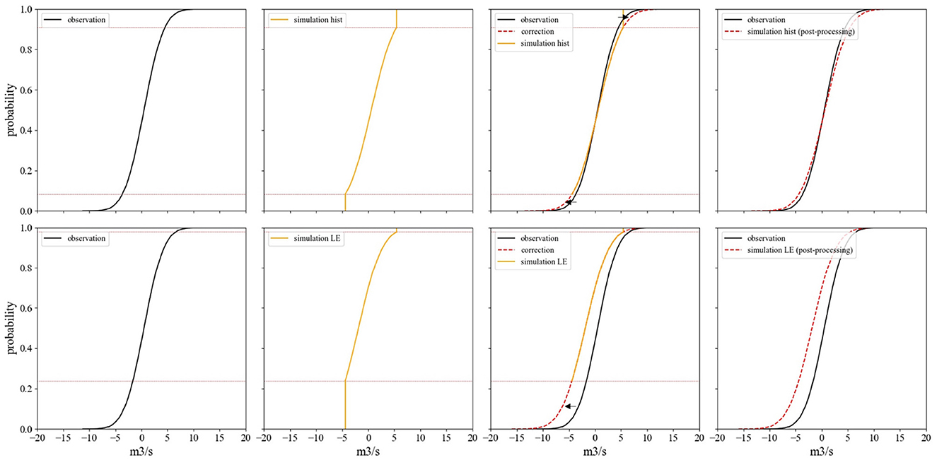
Figure 1. Schematic of post-processing approach based on information of historical observation CDF (black), which is transferred to simulation results (orange) of historical simulations (top) and single ensemble member of simulated target variable based on LE data (bottom). The information regarding tail of the distribution is transferred to simulation results by shifting and extrapolating the simulated tail (black arrow) to the shape of the historical observation one (indicated by red dotted line), resulting in a corrected target value (red, most right).
An example in more detail: while the CDF of the observations (black) would represent values for the probability ranging from 0 to 1, the simulation (orange) would only indicate values corresponding to probabilities of 0.23–0.98, as an example for LE simulation in Figure 1. For the post-processing we take into account the shape of the tail of the observation distribution. This is done by taking the form of the CDF of the observations below the cumulative probability value of the simulated value that represents the cutoff of the lowest observation (0.23 in this case, indicated by the horizontal line in red), if we want to correct for low flows. Furthermore, the number of simulation values that need correction is determined by using the bin count for the lowest simulation value. For the correction the full observation record as well as the full 2000 year simulation data was considered.
The correction step then consists of assigning to each simulated value that needs correcting a value by extrapolating back following the tail of the observed distribution, where the order of assigned values is determined by the order of the simulated values before back transformation (on the 0–1 scale). If the extrapolated tail yields negative values, it is squeezed to fit between zero and the value of the minimum observed value. The same procedure is followed for the upper extreme values of the simulations. The form of the CDF of the observations for range larger than the CDF cutoff value of the simulations is used to extrapolate the simulated values larger than the maximum observed value.
This general post-processing step can be implemented for every location of interest, which allows to include the location specific characteristics by using the station specific observation records to extract the information regarding the distribution tail. This in turn gives the possibility to assess climate change influence at national, regional and local scale. The limitations of the general post-processing step will be discussed in Section 4.
2.2.2. Evaluation
Evaluation of the modeling framework, including the new post-processing steps is validated on historical simulations before applying it to the ensemble simulation results. In this evaluation we specifically focus on the ability of the post-processing routine to reproduce “unseen” events. For this the same modeling framework as in Hauswirth et al. (2021) is used to the test the historic simulations results with and without the post-processing step. The models are trained and tested on a shorter sample of the historical records (1980–2019), with the 20th and 80th percentile of observations representing low and high flows being withheld and thus can be regarded as “unseen” events. The 20th and 80th percentile serve as an example, in other cases the cutoff may be at other percentiles. This example is provided to imitate the situation the models will come across when incorporating the LE for future scenarios (where extreme events will be included that were clearly out of the training set range or outside of the distribution of the observational record). The post-processing step is tested on the periods including most “unseen” events to see whether these low/high flow periods can be recreated by the model, having not seen them in the training phase. The CDFs of the observational records for the validation period, the simulations with and without the additional post-processing step will be assessed to demonstrate the potential of the suggested post-processing approach.
2.3. Analysis of extreme events
For the analysis of extreme events we looked at the change in frequency, average duration, average intensity and number of events for national, regional and local scale. To define low and high flows, the 20th and 80th percentile of the annual discharge was chosen. Regarding frequency, the percentage of discharge that falls into these categories was computed for every month. For average duration, average intensity and number of events a threshold of minimum 7 continuous days was introduced to classify time steps as low or high flow events. The average duration for events in a given month was calculated as the average number of days of extreme events that started in that month (and potentially continued into the following months). The average intensity was computed by including the mean discharge of the extreme events (thus > 7 days above or below a threshold) for the station of interest. The number of events was calculated over the whole ensemble simulations. Furthermore, percentage difference between the scenarios means, 20th and 80th percentiles and standard deviations were computed to assess whether the simulation results were underlying a change in climate variability.
3. Results
The results section will lead from the proof of concept for the post-processing approach to the results of the different climate change scenario simulations. The latter will include a focus on one ML model and the general trends and patterns regarding the different climate change scenarios and their influence on extreme events. Furthermore, the results will be reported first on a national scale, before breaking them down to regional and local results, highlighting a few stations separately. Information and results from different ML models will be listed in the Supplementary material.
3.1. Proof of concept
The proof of concept for the suggested post-processing step is highlighted in Figure 2, where the observations as well as the simulated timeseries of one ML model and one station is shown. The model simulation in blue (Figure 2A), which did not undergo the separate post-processing step, is not able to simulate the low and high flows for this station. This is due to a) having excluded the 20th and 80th percentile in training but also b) the transformer used for the input data is not able to back-transform values that were outside the range of values included in the input data (used to fit the transformer initially). Including the post-processing step, which incorporates information gained from the tail of the observation distribution, corrects the simulation results for the low and high flow periods as seen for the timeseries in red (center panel). The correction for the discharge simulation can furthermore be seen in the right panel including the CDF curves for observations and simulations (with and without correction). The CDF curve of the corrected simulation is following the one of the observations, both in terms of range but also shape. The effect of the post processing on the simulations including the LE are further highlighted in Supplementary Figure S2 for the different scenarios.
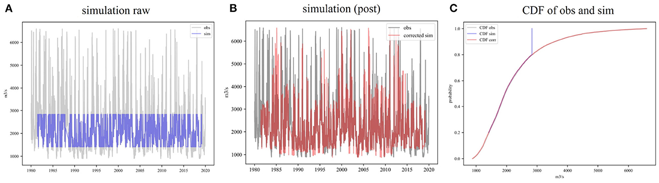
Figure 2. Example station Lobith (MReg model) including the (A) discharge observations (gray) and the simulated discharge (withholding 20th and 80th percentile in training, blue), (B) post-processed discharge simulation (red) and (C) discharge CDF including observations (obs) and simulations (sim), both raw and post.
3.2. Scenario results
The focus of the different scenario results was put on extreme events such as droughts and floods, which were analyzed in terms of their frequency, duration and intensity. Regarding frequency, the discharge percentage that fell into the 20th (low flow), and 80th (high flow) percentile for every month was computed. Figure 3 presents the results based on the average of all the stations and all ML models, therefore representing a national and model average. The low flows are indicated in yellow (present-day, PD), orange (2°C, 2C) and red (3°C, 3C) for the different warming scenarios, the high flows are represented in light blue (PD), blue (2C), and dark blue (3C). The white spacing between the high and low flow bars represents the normal flow (between the 20th and 80th percentile) during the different months.
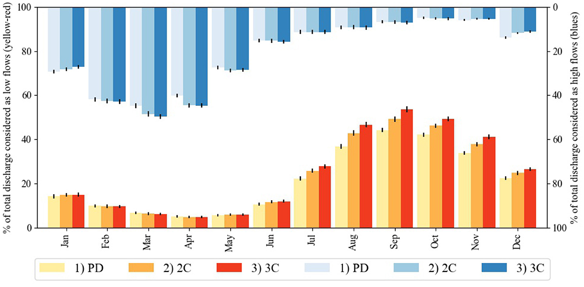
Figure 3. Seasonal cycle of the percentage of time in a month of low and high flows under different scenarios including present day, 2°C and 3°C warmer climate (PD, 2C, and 3C). Low flows are highlighted in yellow (PD), orange (2C) and red (3C), high flows in light blue (PD), blue (2C), and dark blue (3C). Results are averaged over all models for all stations of the study area. Whisker represent 20th and 90th percentile of the uncertainty analysis based on bootstrap calculation of the mean.
For every scenario, it can be seen that low flows occur in all months with varying frequencies. A seasonal cycle can be observed in all scenarios, represented by an increase in low flow frequency throughout summer and autumn (Jun-Sep) with a max of 54% (3C), 49% (2C), and 44% (PD) in Sep compared to earlier in the year. Lowest frequency (~ 5% for all scenarios) in low flow events are showing in early spring, which is due to snow melt dynamics influencing stations along the Rhine, and was also observed in the previous forecasting study by Hauswirth et al. (2022).
Differences between scenarios for the low flow are largest during the second half to the year (Jul-Dec, up to 6% between scenarios), while Jan-May show comparable percentages of discharge falling into the low flow category (up to 0.5%).
Shifting the focus to the seasonal pattern of the high flow events, an increase in high flow frequency throughout Dec-Mar, followed by a decrease during the following months is observed for all scenarios. Highest percentages are seen for Mar with 50% (3C), 48% (2C), and 45% (PD). As can be seen, not only the present day variation in the frequency of high and low flows complement each other, as expected, but also the changes in high and low frequencies under climate change are complementary, showing opposite trends where e.g., lower low flows during Feb and Mar but increased high flow percentages due to shifts in snow melt dynamics.
Smaller changes between the different scenarios are observed in the high flow frequency. Feb, Mar and Apr represent months in which 2C and 3C lead to a higher frequency, however the differences between the latter two are relatively small (1–4%) compared to the ones observed for the low flows (4–6%). Summer and autumn months which show a decline in high flow frequency only indicate minor differences between the scenarios.
The trends and patterns seen for both low and high flows in the different scenarios are due to a change in climate variability, which was found by looking into the mean, 20th and 80th percentile, and standard deviation (also shown in Supplementary Figure S8). While the changes in the mean discharge under 2C and 3C lies below 5% compared to the PD scenario for the large majority of the stations, the changes regarding the low flows (20th percentile) range between 10 and 20%. Analysis of the simulation results of the different ML models (Supplementary Figures S4–S7) indicates that the direction and magnitude of trends and changes is similar across the methods. The absolute frequency between the different ML methods differ but the direction of change is similar for all models. Due to the large amount of data provided by the LE the changes seen are statistically significant. We additionally incorporated an uncertainty analysis based on the bootstrap approach, where we included the national and model average data and calculated the mean after randomly dropping 10% of the data for each month and scenario. This was repeated 1,000 times. From the selection of means, the 10th and 90th percentile were chosen for the whiskers, which are represented in Figure 3 in black. Regarding model forcing, it was not possible to assess the GCM uncertainty as only one LE with this magnitude was available.
The increasing severity of low flows in different months was also evaluated in terms of duration, number of events and average intensity. Figure 4A presents the average event duration based on the starting month of the low flow events. Early spring to autumn show an increase in average duration distribution for different months but also between the scenarios, with the 3C indicating the largest variation (Jul, 9–27 days). Differences in median duration between scenarios are minor during winter months and start to increase in May-Sep (14 days, July, 3C). Largest variations are observed in the 90th percentile (May, 70 days - Nov, 30 days), with largest differences between scenarios in month Jun and Jul. The increase in average duration (seen in the distribution but also the 90th percentile) leads to events which are overlapping with the following months, which corresponds to the higher low flow percentage observed in Figure 3 for the summer and autumn months. The number of events seen in Figure 4B show the same seasonal pattern as observed in Figure 3. While Jan-May show similar number of events for all scenarios, clear differences are observed for summer and autumn months with 3C showing the highest number of events. In terms of average intensity (Figure 4C), differences in median intensity are small throughout all months and scenarios. However, the largest variation of average intensity is found for months Feb–May, which are also the months with the lowest number of events.
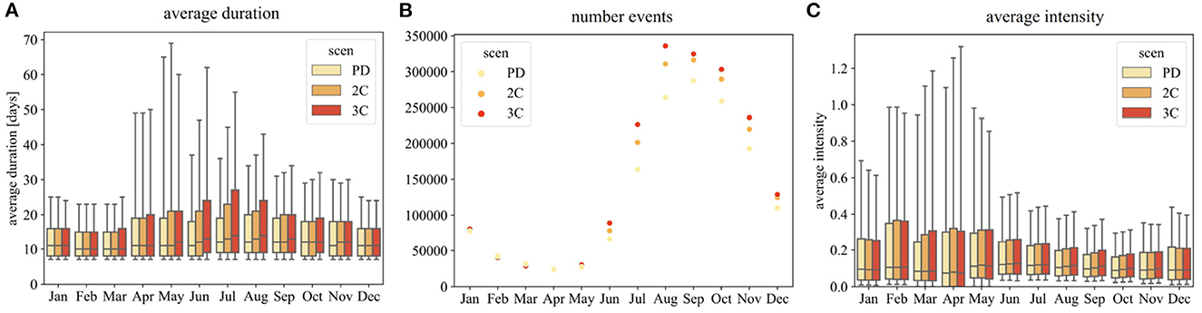
Figure 4. (A) Average low flow duration, (B) number of events and (C) average intensity based on different months in which low flow periods started for PD, 2C and 3C scenario (based on national and model average). Low flow events are defined by the 20th percentile threshold, lasting a minimum of 7 days. The number of events is total over the full ensemble in a scenario. Average intensity is normalized by the annual mean discharge of the stations included. Whiskers represent 10th and 90th percentile.
Focusing on the national scale for assessing the differences in scenario results show that both high and low flow percentages represent a seasonal cycle with increased low flow frequency during summer and autumn months, while high flow frequencies are increasing during (early) spring months.
3.3. Spatial characteristics-regionally
Moving from the national scale to a more regional assessment, Figure 5 shows the averaged results for stations of 5 different regions based on the model input of the LSTM model and the same data analysis used as in Figure 3.
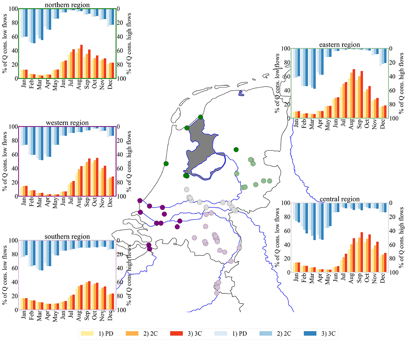
Figure 5. Seasonal cycle of percentage of low and high flows under different scenarios PD, 2C and 3C, averaged over different regions (indicated by the group of dots with same color) based on the LSTM model results. Regions are defined into northern (dark green), eastern (light green), central (gray), southern (light pink) region and western (purple) region. Major rivers are presented by blue lines, while the dark gray area represents the IJsselmeer lake. Low flows are highlighted in yellow (PD), orange (2C), and red (3C), high flows in light blue (PD), blue (2C), and dark blue (3C).
Focusing on low flow frequency first, a similar underlying pattern in terms of seasonal low flows can be observed as for the national average (Figure 3). Compared to the latter, shifts in terms of an earlier increase in low flow frequency (northern and eastern region), as well as higher maximum percentages (central: ~58%, eastern: ~70%, northern: ~48%, and western region: ~55% for 3C) is observed. Furthermore, the differences between the scenarios are more pronounced, especially for the summer months for which increased low flow percentages are recorded.
The central region is strongly influenced by incoming Rhine discharge, which was also seen in previous work by Hauswirth et al. (2021). Compared to the national average, spring months including Apr and May show a lower percentage of low flows for these months, likely due to the snow melt signal captured in the Rhine discharge. However, regions which are also linked to the Rhine (eastern, northern and western) show a stronger and earlier increase in low flows as well as decrease in the winter (Nov, Dec, Jan, Feb).
The southern region, which is predominantly fed by the Meuse discharge, also shows an increase in low flow frequency during the summer months. However, the maximum percentages observed are lower (~41% in Sep, 3C) and furthermore, a relatively high percentage of ~15% is already observed in Jan-Mar, which might be due to the Meuse being a rain water system where the snow melt dynamic signal is missing.
The differences observed between the regions and the main Rhine discharge can furthermore be seen in more detail in Supplementary Figure S3, where the regional difference are presented relative to the “base” station at Lobith (Rhine observations which were used as input variable in previous studies).
If the focus is shifted toward the high flow percentages in Figure 5, similar observations regarding shifts and differences between the regions can be made as for low flow periods, as well as the underlying seasonality which corresponded to the national average in Figure 3. The central, eastern, northern and western region indicate a stronger and earlier increase in high flows during the first few months of the year with Mar and Apr showing the highest percentages (53%, 58%, 50%, and 48% for 3C). For the northern and eastern regions high flow percentages are lowest during summer months, while in other regions they vary around ~3%. The southern region shows a less pronounced seasonal cycle than the other regions, with a lower maximum high flow percentage around ~43% for both warming scenarios in Mar.
In general, the largest increase in frequencies with warming are observed for the low flows, while the changes in high flow frequency are less pronounced and much closer to the PD for most months. More details regarding the differences of the regions compared to the “base” station Lobith can furthermore be seen in Supplementary Figure S3.
The results shown in Figure 5 and supported by Supplementary Figure S3 showed that we are able to capture regional differences with locally informed models. These regional differences can also be seen for the other ML models (see Supplementary material including Supplementary Figures S4–S7).
3.4. Spatial characteristics-locally
Using the ML model framework based on local models allowed to assess the influence of climate change on extreme events also on a local scale, next to the national and regional already previously elaborated. Figure 6 shows the result for high and low flow frequency for the different scenarios (same approach as in previous Figures 3, 5) for a selection of stations throughout the Netherlands. Some stations are located along the main river network, others at smaller streams (not drawn on the map).
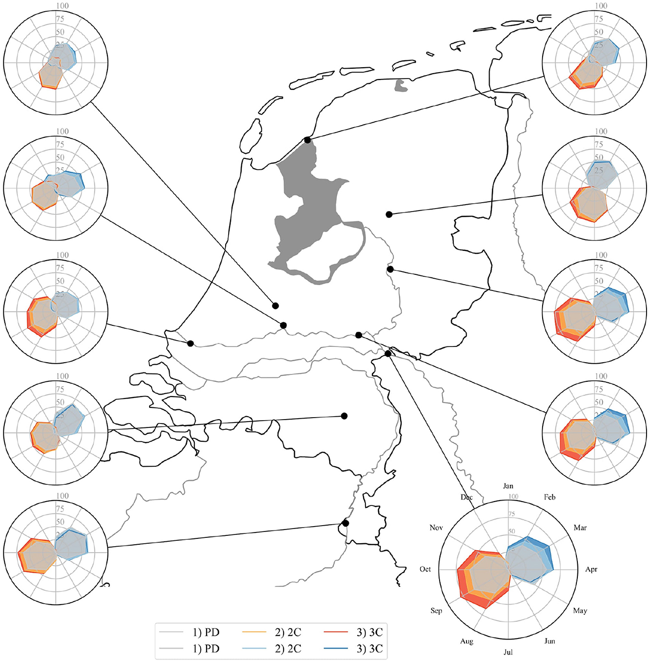
Figure 6. Seasonal patterns in percentage of low and high flows for different stations and scenarios PD, 2C, and 3C, based on results from LSTM model. PD values for both high and low flows are represented by the gray shaded areas. Low flows for 2C are highlighted in orange and for 3C in red. High flows for 2C are shown in blue and dark blue (3C).
Looking at the station represented by the bottom right, enlarged radar plot as an explanatory example, the percentages for both high and low flows are represented by the shaded shape for each scenario in corresponding colors throughout the year (PD in gray, 2C orange/light blue, 3C red/blue).
For both changes in low and high flows we observe similar trends as on the national and regional scale, albeit with more local details. For the example station at Lobith (bottom right) we see that the frequency of low flow events for all scenarios increases from Jul-Sep, while high flows increased in the period Jan to Apr.
Other stations highlighted in Figure 6 show similar patterns as the example station in terms of the shape of the different scenario results. Some station vary in the shift of these shapes (most northern ones), indicating that the high and low flow periods are starting earlier in the year, or also in terms of frequency. For example, stations located in the southern region show lower frequencies in terms of maximum high flows and furthermore the differences between the scenarios are smaller. Minor differences between scenarios but larger deviations in terms of frequency compared to other stations are also observed (top two left stations). Most of these observations regarding shifts and differences in frequencies were already found in the regional assessment, however more detailed patterns and exceptions were now able to be explored.
The shifts observed for the different stations are also observed in the mean, the 20th and 80th (Supplementary Figure S8), which indicates that the trends and patterns seen for the different scenarios are due to a change in the mean climate and its variability. Shifts in the mean range between ± 10% for most stations compared to the PD scenario, with the largest shifts seen for stations with low mean annual discharge. Shifts in low flow extremes range up to 20%, while high flow events show a smaller range (± 10%). This indicates that the changes in climate variability will have the most significant impact on low and high flows in the Netherlands.
Overall, for both high and low flows the differences in shifts for the different stations correspond well to the shifts found in the respective regions the station is located in. However, analysing the results of the stations also showed that frequencies and changes in frequencies can be locally slightly different from the regional average. This shows that having a locally trained ML framework is useful for bringing large scale information, such as the large climate ensembles, to local scale and therefore making it possible to assess future changes under changing climate and the adaptation requirements more location specific.
4. Discussion
This study combined a locally trained ML model framework with global LE with the goal to see if and how they can be combined to assess extreme events under different warming levels (PD, 2C, and 3C) to potentially create valuable local estimates of climate change impacts from large-scale inputs.
Due the setup of the ML model framework including a simple, exchangeable input dataset, the incorporation of the LE was straightforward, similar to the previous study using the same model framework for seasonal forecasting by incorporating seasonal reforecasting data as input (Hauswirth et al., 2022). The locally trained models inherit information on the discharge characteristics for each station, translating large scale information to regional and even scales which are deemed relevant for adaptation measures. Especially in terms of climate change assessment, this can be of big interest as most of these assessments are based on large scale trends. The LE used in this study create a new opportunity to assess climate change and extreme events for different warming scenarios, compared to the more traditional approach including stochastic or GCM+GHM models where only one non-stationary timeseries is given. The ensemble approach provides orders of magnitude more realizations of extreme events, compared to more classic CMIP6 type transient climate simulations (van der Wiel et al., 2019b). At the same time, LE simulations allow to identify the hydrological impact of specific warming levels. LE have already proven to be relevant for impact assessment in for example energy production or agriculture (van der Wiel et al., 2019a; Goulart et al., 2021). In this study we showed that by combining LE with a local ML modeling framework enables us to project local hydrological effects of climate change which gives water management a more detailed outlook on potential direct impacts on flood risk and available water resources in the future.
To make extrapolation in a ML model framework possible, a new post-processing approach was introduced. The suggested non parametric post-processing step in this study underlies the assumption that the tails of the distribution (representing extreme events) of the historical observations for each station remain the same for future events. This approach is relatively simple, can be implemented readily without needing high computational demand and brings the added benefit of being location specific and therefore creating the opportunity to scale down possible effects of climate change. However, it is dependent on having a long observational record for locations of interest. Due to extreme events having large return times and observational records not always being available or not long enough (in our case 30 years) this of course can lead to the post-processing step not correcting for the full scale of the extreme events in the LE. Furthermore, the form of the tails of the probability distribution of future events might be changing and therefore our assumption might not hold. However, this simple post-processing step is a first step to a fully data-based approach to simulating future extreme events. Assuming that the form of the tails above and below the training data values remains the same has its limitations, but is not better or worse than assuming some parametric form for extrapolation. Also using the statistical information of modeled data from physically based models has its limitations as they inherently also make assumptions and as such are also biased in their reproduction of the tail (and with a significantly higher computation demand). Using ML models trained on historic local observations gave us models that are closer to the original observations, compared to having models trained and tested on data obtained from future projections with physically-deterministic model forced with the LE. It remains to be seen if a physically based model is closer to the unknown future than our ML method with post-processing. The proof of concept showed that the approach taken in this work provided a reasonable solution for the inherit extrapolation problem in ML based future projections. Even though the most extreme events might not be able to be reconstructed with this method, the general trend and patterns, especially for long term events such as drought, can still be simulated and therefore gives a base for climate change assessments on a local scale.
The trends observed in this study are in line with earlier work projecting changes in hydrological extremes for the river Rhine. However, the approach used here allows for further downscaling of the results, bringing the relevant information and insights to a more local level and making them more applicable for decision makers. This can be of interest to local authorities who are in need of locally specific information, as studies regarding climate change are often on a larger scale. Changes observed between the different scenarios were likely due to a change in climate variability. The discharge simulation (based on LE and PCRGLOBWB) incorporated in the input data for the ML framework did include a shift in the extreme events and the mean, which was also present in the input data after bias correction. We observed that this information was also found in simulated discharge for the different stations. While the shifts in the mean for the stations were between ± 10%, shifts in the extreme events (especially low flow periods) could reach up to 20%. This is in line with previous assessments at the national scale suggesting that climate change will be more prominently felt in shifts in the extremes than in the average climate.
5. Conclusion
In this study, large climate ensembles (LE) and local, observation based hydrological machine learning (ML) models were combined to assess extreme events under different warming scenarios [present-day (PD), 2°C (2C), and 3°C (3C) warmer climate]. The incorporation of LE, which in our case consisted of 2000 years of global data for every scenario, provided the opportunity to be able to empirically assess extreme events due to the large number of realizations of future weather. Combining this information with local ML models allowed for detailed and local, regional and national estimates of future hydrological extremes, therewith creating locally specific information that is of interest to local water managers.
A new post-processing approach based on historical information was introduced to enable the projections of extreme values outside the observed data range and incorporate the LE for local assessments of extreme events. The application of the post-processing step was tested on historical simulations first before being implemented for the different warming scenarios.
Extreme event analysis at the national scale in terms of discharge low and high flows for the different climate change scenarios and spatial scale showed a clear seasonal cycle with increased low flow periods from summer till the end of autumn (~45% average for August–October) and increased high flow periods for early spring (~43% average for February–April). Highest frequencies of low flow periods were reached with the 3C climate scenario showing the highest percentages for both type of events (53 and 50% respectively). Regional differences were seen in terms of shifts (low flows occurring earlier in the year) and ranges (higher/lower percentages). These trends, albeit with slightly different values, were further detangled into location specific results.
Differences in extremes between the different scenarios were predominantly due to a change in climate variability, which was seen by analysing the mean, the 20th and 80th for different discharge stations. Largest shifts regarding the mean were observed for stations with low annual mean discharge, while shifts in extreme events such as low flow were seen for all.
In this study we show that by combining the wealth of information from large climate ensembles, local characteristics captured locally with observation-based ML models and a suitable post-processing method for tail extrapolation allows the projection of future extremes under climate change. The local modeling framework thus provides important information for local to regional water management to be used in long term planning.
Data availability statement
The raw data supporting the conclusions of this article will be made available by the authors, without undue reservation.
Author contributions
Conceptualization of this research has been done by SH, NW, MB, KvdW, and VB. Climate data acquisition was done by KvdW. Hydrological data acquisition was done by SH. Data analysis was performed by SH, with input from NW and MB. Writing was done by SH with feedback by NW, MB, KvdW, and VB. All authors contributed to the article and approved the submitted version.
Funding
SH acknowledges funding from the Corporate Innovation Program and the Department of Water, Transport and Environment at the Dutch National Water Authority, Rijkswaterstaat. NW acknowledges funding from NWO 016.Veni.181.049.
Acknowledgments
Figure maps were created using the python package Cartopy (Elson et al., 2022), which uses basemap data from Made with Natural Earth and © OpenStreetMap contributors 2022. Distributed under the Open Data Commons Open Database License (ODbL) v1.0.
Conflict of interest
The authors declare that the research was conducted in the absence of any commercial or financial relationships that could be construed as a potential conflict of interest.
Publisher's note
All claims expressed in this article are solely those of the authors and do not necessarily represent those of their affiliated organizations, or those of the publisher, the editors and the reviewers. Any product that may be evaluated in this article, or claim that may be made by its manufacturer, is not guaranteed or endorsed by the publisher.
Supplementary material
The Supplementary Material for this article can be found online at: https://www.frontiersin.org/articles/10.3389/frwa.2023.1108108/full#supplementary-material
References
Bardsley, W., Vetrova, V., and Liu, S. (2015). Toward creating simpler hydrological models: a LASSO subset selection approach. Environ. Model. Software 72, 33–43. doi: 10.1016/j.envsoft.2015.06.008
de Bruin, H. A. R., and Lablans, W. N. (1998). Reference crop evapotranspiration determined with a modified Makkink equation. Hydrol. Processes 12, 1053–1062. doi: 10.1002/(SICI)1099-1085(19980615)12:7andlt;1053::AID-HYP639andgt;3.0.CO;2-E
Deser, C., Lehner, F., Rodgers, K. B., Ault, T., Delworth, T. L., DiNezio, P. N., et al. (2020). Insights from Earth system model initial-condition large ensembles and future prospects. Nat. Clim. Chang 10, 277–286. doi: 10.1038/s41558-020-0731-2
Elson, P., de Andrade, E. S., Lucas, G., May, R., Hattersley, R., Campbell, E., et al. (2022). SciTools/cartopy: v0.20.2 (v0.20.2). Zenodo. doi: 10.5281/zenodo.6775197
Felsche, E., and Ludwig, R. (2021). Applying machine learning for drought prediction in a perfect model framework using data from a large ensemble of climate simulations. Natural Hazards Earth Syst. Sci. 21, 3679–3691. doi: 10.5194/nhess-21-3679-2021
Fowler, H. J., Blenkinsop, S., and Tebaldi, C. (2007). Linking climate change modelling to impacts studies: recent advances in downscaling techniques for hydrological modelling. Int. J. Climatol. 27, 1547–1578. doi: 10.1002/joc.1556
Giorgi, F. (2019). Thirty years of regional climate modeling: where are we and where are we going next? J. Geophys. Res. Atmosph. 124, 5696–5723. doi: 10.1029/2018JD030094
Goulart, H. M. D., van der Wiel, K., Folberth, C., Balkovic, J., and van den Hurk, B. (2021). Storylines of weather-induced crop failure events under climate change. Earth Syst. Dyn. 12, 1503–1527. doi: 10.5194/esd-12-1503-2021
Graham, L. P., Andréasson, J., and Carlsson, B. (2007). Assessing climate change impacts on hydrology from an ensemble of regional climate models, model scales and linking methods - a case study on the Lule River basin. Clim. Change 81, 293–307. doi: 10.1007/s10584-006-9215-2
Hauswirth, S. M., Bierkens, M. F., Beijk, V., and Wanders, N. (2021). The potential of data driven approaches for quantifying hydrological extremes. Adv. Water Resour. 155, 104017. doi: 10.1016/j.advwatres.2021.104017
Hauswirth, S. M., Bierkens, M. F. P., Beijk, V., and Wanders, N. (2022). The suitability of a hybrid framework including data driven approaches for hydrological forecasting. Hydrol. Earth Syst. Sci. Discuss. 27, 501–517. doi: 10.5194/hess-2022-89
Hazeleger, W., Wang, X., Severijns, C., Ştefănescu, S., Bintanja, R., Sterl, A., et al. (2012). EC-Earth V2.2: description and validation of a new seamless earth system prediction model. Clim. Dyn. 39, 2611–2629. doi: 10.1007/s00382-011-1228-5
Hochreiter, S., and Schmidhuber, J. (1997). Long Short-Term Memory. Neural Comput. 9, 1735–1780. doi: 10.1162/neco.1997.9.8.1735
Kelder, T., Wanders, N., Wiel, K. v. d, Marjoribanks, T. I., Slater, L. J., et al. (2022). Interpreting extreme climate impacts from large ensemble simulations–are they unseen or unrealistic? Environ. Res. Lett. 17, 044052. doi: 10.1088/1748-9326/ac5cf4
Koch, J., Gotfredsen, J., Schneider, R., Troldborg, L., Stisen, S., and Henriksen, H. J. (2021). High resolution water table modeling of the shallow groundwater using a knowledge-guided gradient boosting decision tree model. Front. Water 3, 701726. doi: 10.3389/frwa.2021.701726
Kratzert, F., Klotz, D., Brenner, C., Schulz, K., and Herrnegger, M. (2018). Rainfall-runoff modelling using long short-term memory (LSTM) networks. Hydrol. Earth Syst. Sci. 22, 6005–6022. doi: 10.5194/hess-22-6005-2018
Maher, N., Milinski, S., and Ludwig, R. (2021). Large ensemble climate model simulations: introduction, overview, and future prospects for utilising multiple types of large ensemble. Earth Syst. Dyn. 12, 401–418. doi: 10.5194/esd-12-401-2021
Mai, J., Shen, H., Tolson, B. A., Gaborit, E., Arsenault, R., Craig, J. R., et al. (2022). The great lakes runoff intercomparison project phase 4: the great lakes (GRIP-GL). Hydrol. Earth Syst. Sci. 26, 3537–3572. doi: 10.5194/hess-26-3537-2022
Masson-Delmotte, V., Zhai, P., Pirani, A., Connors, S. L., Péan, C., Berger, S., et al. (2022). “IPCC, 2021: summary for policymakers,” in Climate Change 2021: The Physical Science Basis. Contribution of Working Group I to the Sixth Assessment Report of the Intergovernmental Panel on Climate Change. Technical report (Cambridge, UK; New York, NY: Cambridge University Press).
Milly, P. C. D., Dunne, K. A., and Vecchia, A. V. (2005). Global pattern of trends in streamflow and water availability in a changing climate. Nature 438, 347–350. doi: 10.1038/nature04312
Pachauri, R. K., Mayer, L., and on Climate Change, I. P. (Eds.). (2015). Climate change 2014: Synthesis Report. Geneva: Intergovernmental Panel on Climate Change.
Rummukainen, M. (2010). State-of-the-art with regional climate models. WIREs Clim. Change 1, 82–96. doi: 10.1002/wcc.8
Samaniego, L., Thober, S., Kumar, R., Wanders, N., Rakovec, O., Pan, M., et al. (2018). Anthropogenic warming exacerbates European soil moisture droughts. Nat. Clim. Chang 8, 421–426. doi: 10.1038/s41558-018-0138-5
Sutanudjaja, E. H., van Beek, R., Wanders, N., Wada, Y., Bosmans, J. H. C., Drost, N., et al. (2018). PCR-GLOBWB 2: a 5 arcmin global hydrological and water resources model. Geosci. Model Dev. 11, 2429–2453. doi: 10.5194/gmd-11-2429-2018
van der Wiel, K., Batelaan, T. J., and Wanders, N. (2022). Large increases of multi-year droughts in north-western Europe in a warmer climate. Clim. Dyn. doi: 10.1007/s00382-022-06373-3
van der Wiel, K., and Bintanja, R. (2021). Contribution of climatic changes in mean and variability to monthly temperature and precipitation extremes. Commun. Earth Environ. 2, 1–11. doi: 10.1038/s43247-020-00077-4
van der Wiel, K., Lenderink, G., and de Vries, H. (2021). Physical storylines of future European drought events like 2018 based on ensemble climate modelling. Weather Clim. Extremes 33, 100350. doi: 10.1016/j.wace.2021.100350
van der Wiel, K., Selten, F. M., Bintanja, R., Blackport, R., and Screen, J. A. (2020). Ensemble climate-impact modelling: extreme impacts from moderate meteorological conditions. Environ. Res. Lett. 15, 034050. doi: 10.1088/1748-9326/ab7668
van der Wiel, K., Stoop, L. P., van Zuijlen, B. R. H., Blackport, R., van den Broek, M. A., and Selten, F. M. (2019a). Meteorological conditions leading to extreme low variable renewable energy production and extreme high energy shortfall. Renewable Sustain. Energy Rev. 111, 261–275. doi: 10.1016/j.rser.2019.04.065
van der Wiel, K., Wanders, N., Selten, F. M., and Bierkens, M. F. P. (2019b). Added value of large ensemble simulations for assessing extreme river discharge in a 2°C warmer world. Geophys. Res. Lett. 46, 2093–2102. doi: 10.1029/2019GL081967
Vörösmarty, C. J., McIntyre, P. B., Gessner, M. O., Dudgeon, D., Prusevich, A., Green, P., et al. (2010). Global threats to human water security and river biodiversity. Nature 467, 555–561. doi: 10.1038/nature09440
Keywords: machine learning, large climate ensembles, extreme events, climate change, droughts, floods, global-local
Citation: Hauswirth SM, van der Wiel K, Bierkens MFP, Beijk V and Wanders N (2023) Simulating hydrological extremes for different warming levels–combining large scale climate ensembles with local observation based machine learning models. Front. Water 5:1108108. doi: 10.3389/frwa.2023.1108108
Received: 25 November 2022; Accepted: 01 March 2023;
Published: 21 March 2023.
Edited by:
Dan Lu, Oak Ridge National Laboratory (DOE), United StatesReviewed by:
Sanjiv Kumar, Auburn University, United StatesAlison L. Kay, UK Centre for Ecology and Hydrology (UKCEH), United Kingdom
Copyright © 2023 Hauswirth, van der Wiel, Bierkens, Beijk and Wanders. This is an open-access article distributed under the terms of the Creative Commons Attribution License (CC BY). The use, distribution or reproduction in other forums is permitted, provided the original author(s) and the copyright owner(s) are credited and that the original publication in this journal is cited, in accordance with accepted academic practice. No use, distribution or reproduction is permitted which does not comply with these terms.
*Correspondence: Sandra M. Hauswirth, cy5tLmhhdXN3aXJ0aEB1dS5ubA==