 Katharina Wilbrand1†
 Riccardo Taormina1*†
 Marie-Claire ten Veldhuis1
 Martijn Visser2
 Markus Hrachowitz1
 Jonathan Nuttall3
 Ruben Dahm4
- 1Department of Water Management, Faculty of Civil Engineering and Geosciences, Delft University of Technology, Delft, Netherlands
- 2Department of Water Resources Management, Deltares, Delft, Netherlands
- 3Department of Geotechnics and Flood Defenses Software, Deltares, Delft, Netherlands
- 4Department of Catchment and Urban Hydrology, Deltares, Delft, Netherlands
Streamflow predictions remain a challenge for poorly gauged and ungauged catchments. Recent research has shown that deep learning methods based on Long Short-Term Memory (LSTM) cells outperform process-based hydrological models for rainfall-runoff modeling, opening new possibilities for prediction in ungauged basins (PUB). These studies usually feature local datasets for model development, while predictions in ungauged basins at a global scale require training on global datasets. In this study, we develop LSTM models for over 500 catchments from the CAMELS-US data base using global ERA5 meteorological forcing and global catchment characteristics retrieved with the HydroMT tool. Comparison against an LSTM trained with local datasets shows that, while the latter generally yields superior performances due to the higher spatial resolution meteorological forcing (overall median daily NSE 0.54 vs. 0.71), training with ERA5 results in higher NSE in most catchments of Western and North-Western US (median daily NSE of 0.83 vs. 0.78). No significant changes in performance occur when substituting local with global data sources for deriving the catchment characteristics. These results encourage further research to develop LSTM models for worldwide predictions of streamflow in ungauged basins using available global datasets. Promising directions include training the models with streamflow data from different regions of the world and with higher quality meteorological forcing.
1. Introduction
Streamflow Prediction in Ungauged Basins (PUB) is a major challenge in hydrology due to a lack of streamflow observations required for calibration and validation of hydrological models. Worldwide, the availability of streamflow observations is unbalanced with a rather high abundance in North America and Europe and very scarce data in African, Asian, and South American river basins. These data scarce regions would benefit greatly from models calibrated against streamflow observations available elsewhere that can generalize to poorly gauged or ungauged catchments. Over the last decades, the PUB initiative (Sivapalan et al., 2003; Hrachowitz et al., 2013) highlighted the need to transfer hydrological process understanding from gauged to ungauged catchments. This led to the development of many methods for model regionalization (Merz and Blöschl, 2004; Götzinger and Bárdossy, 2007; Samaniego et al., 2010). However, the fundamental underlying problem concerning hydrological similarity remains largely unresolved. As long as there is no general and meaningful answer, regionalization of process-based models will be characterized by considerable uncertainties. As a consequence, and in spite of some recent promising advances (Kumar et al., 2013; Gao et al., 2016), it is unclear which processes, associated parametrizations, and actual parameter values are necessary for the most suitable representation of the hydrological processes at any given location, as recently demonstrated by Bouaziz et al. (2021) and Gharari et al. (2021). This complicates the transfer of calibrated models to ungauged locations.
Data-driven approaches such as deep learning (DL) algorithms, in contrast, quantify the relations between meteorological input and streamflow output directly from the data without any further assumptions. Recently, the application of Long Short-Term Memory (LSTM) architecture developed by Hochreiter and Schmidhuber (1997) achieved high performance for streamflow predictions across the US (Kratzert et al., 2018; Shen, 2018; Fang et al., 2020; Gauch et al., 2021; Lees et al., 2021), outperforming traditional conceptual/physical models (Kratzert et al., 2018; Mai et al., 2022; Arsenault et al., 2023). In particular, LSTM show better out-of-sample prediction when trained on large-sample datasets including time series of streamflow observations (outputs) and meteorological forcing (dynamic inputs) as well as catchment characteristics (static inputs) (Kratzert et al., 2018; Shen, 2018; Lees et al., 2021). It can be expected that a larger training catchment variety yields more general applicability of the relationships between meteorological input and streamflow at the catchment outlet, an important precondition for PUB (Fang et al., 2022). Indeed, from a machine learning perspective, PUB entails working in a “zero-shot” regime, i.e., performing predictions with direct transfer learning without explicit retraining on streamflow data from the target catchment (Oreshkin et al., 2021).
Several studies tested the transferability of LSTM models trained on multiple catchments to out-of-sample catchments to evaluate the suitability of this approach for PUB. Kratzert et al. (2019a) trained an LSTM model on catchments of various climate zones in the US and achieved high NSE values for independent, out-of-sample US catchments. Ayzel et al. (2020) reached similarly good performance for out-of-sample testing in Russian catchments. Ma et al. (2021) tested the global transferability of LSTM models to catchments with limited streamflow data for recalibration. They pre-trained an LSTM model on US catchments, fine-tuned it for Chilean, British, and Chinese catchments based on short time series of a few years, and achieved good prediction performance. Ma et al. (2021), thereby, reveal indicators for hydrological similarity, i.e., commonalities of hydrological behavior, across continents that is detectable with LSTM models. However, their transfer strategy always requires local forcing and streamflow data to fine-tune (re-calibrate) it to the catchment of interest.
All the aforementioned studies resorted to local high spatial resolution datasets for model development, which limit their application to other regions of the world. Developing LSTM models using global datasets may have the potential to facilitate transferability to catchments worldwide, particularly in regions where no high-resolution local datasets are available. The overall objective of this study is thus to analyze the potential of global datasets to train LSTM models for streamflow prediction. Specifically, we develop LSTM models with ERA5 meteorological data and HydroMT catchment characteristics for over 500 US catchments, and we compare their performance with LSTM developed with local datasets. To further investigate the differences in predictive performances between global and local datasets, we also trained mixed LSTM models, where global meteorological forcing was used as inputs along with local catchment characteristics and vice-versa.
2. Materials and methods
We perform the analysis using the Multi-Timescale LSTM (MTS-LSTM) (Gauch et al., 2021) architecture for catchments across the US. The MTS-LSTM can predict streamflow at sub-daily temporal resolution of interest for applications such as flood prediction. We chose the global ERA5 reanalysis dataset as the meteorological forcing dataset, as it was shown to have explanatory power for hydrological predictions comparable to that of local in-situ observations in an analysis for US catchments (Tarek et al., 2020). Furthermore, ERA5 has a continuous coverage since 1970 and is available on an hourly basis, a prerequisite to serve as input for the MTS-LSTM. We resort to the HydroMT tool to retrieve global catchment characteristics (Eilander et al., 2023).
2.1. Data
2.1.1. Streamflow data
We have chosen 516 catchments with areas of < 2000 km2 distributed across the United States, covering several climate zones with more than three decades of daily streamflow observations. These catchments are a subset of the Catchment Attributes and Meteorology for Large-sample Studies (CAMELS) US dataset used by Gauch et al. (2021). As the CAMELS-US dataset only includes streamflow observations on daily time-steps, we use the streamflow data from the United States Geological Survey (USGS) Water Information System, pre-processed by Gauch et al. (2021) to hourly and daily time-series over the period from 1 October 1980 to 30 September 2018.
2.1.2. Meteorological forcing
For the local model, we employ the North American Land Data Assimilation System Phase 2 (NLDAS-2) local meteorological dataset, which provides hourly data for 11 different forcing variables from 1980 to 2018, with a spatial resolution of approximately 12 km (i.e., 0.125 degree) (Xia et al., 2012). NLDAS-2 precipitation is based on temporal disaggregation of daily field observations supported with disaggregation-weights derived from hourly radar precipitation estimates (Xia et al., 2012). For the global model, we selected the ERA5 dataset. The ERA5 dataset is the climate reanalysis (fifth generation) of the European Centre for Medium-Range Weather Forecasts (ECMWF), providing atmospheric variables with global coverage. All variables are available from 1980 to 2018 (Hersbach et al., 2020). ERA5 has a resolution of approximately 31 km (i.e., 0.25-degree) and provides forcing time series at hourly time steps. Table 1 shows all 11 forcing variables included in the NLDAS-2 and ERA5 datasets and used in the subsequent analysis.
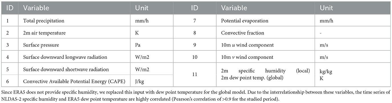
Table 1. Forcing variables available from the local dataset NLDAS-2 and the global dataset ERA5.
2.1.3. Catchment characteristics
Catchment characteristics describe the physical properties of each catchment. Their use yields as static inputs yield better model predictions, also for unseen catchments (Kratzert et al., 2019a; Yin et al., 2021). The CAMELS-US dataset provides a range of catchment characteristics describing climate, topography, soil, land, cover and streamflow (Addor et al., 2017). Although the CAMELS-US dataset is spatially limited to the US, some attributes are derived from datasets with global coverage. Nevertheless, we refer to all attributes derived from CAMELS-US as local catchment characteristics. To work on a global scale, we resort to the HydroMT tool, which employs global raster datasets to derive equal or similar attributes as those included in the local dataset (Eilander et al., 2023).
Table 2 shows 21 characteristics we used as static inputs for the LSTM models along with the underlying data sources, ordered based on the model sensitivity reported by Kratzert et al. (2019a). Some catchment characteristics are statistics derived from the meteorological forcing, such as the average annual precipitation or high precipitation frequency. While these dependent attributes repeat information that is already included in the meteorological forcing inputs, they are usually provided to the models due to their high sensitivity. On the contrary, we excluded some attributes related to soil composition which have been employed in the study by Kratzert et al. (2019a) and other studies because they could not be retrieved from HydroMT. These attributes have relative low sensitivity, and they repeat information contained in the Saturated Hydraulic Conductivity catchment characteristic. This characteristic is determined with pedo-transfer functions in HydroMT (Imhoff et al., 2020), while CAMELS-US reports the estimates of multiple regression relying on sand and clay fractions from the study by Cosby et al. (1984).
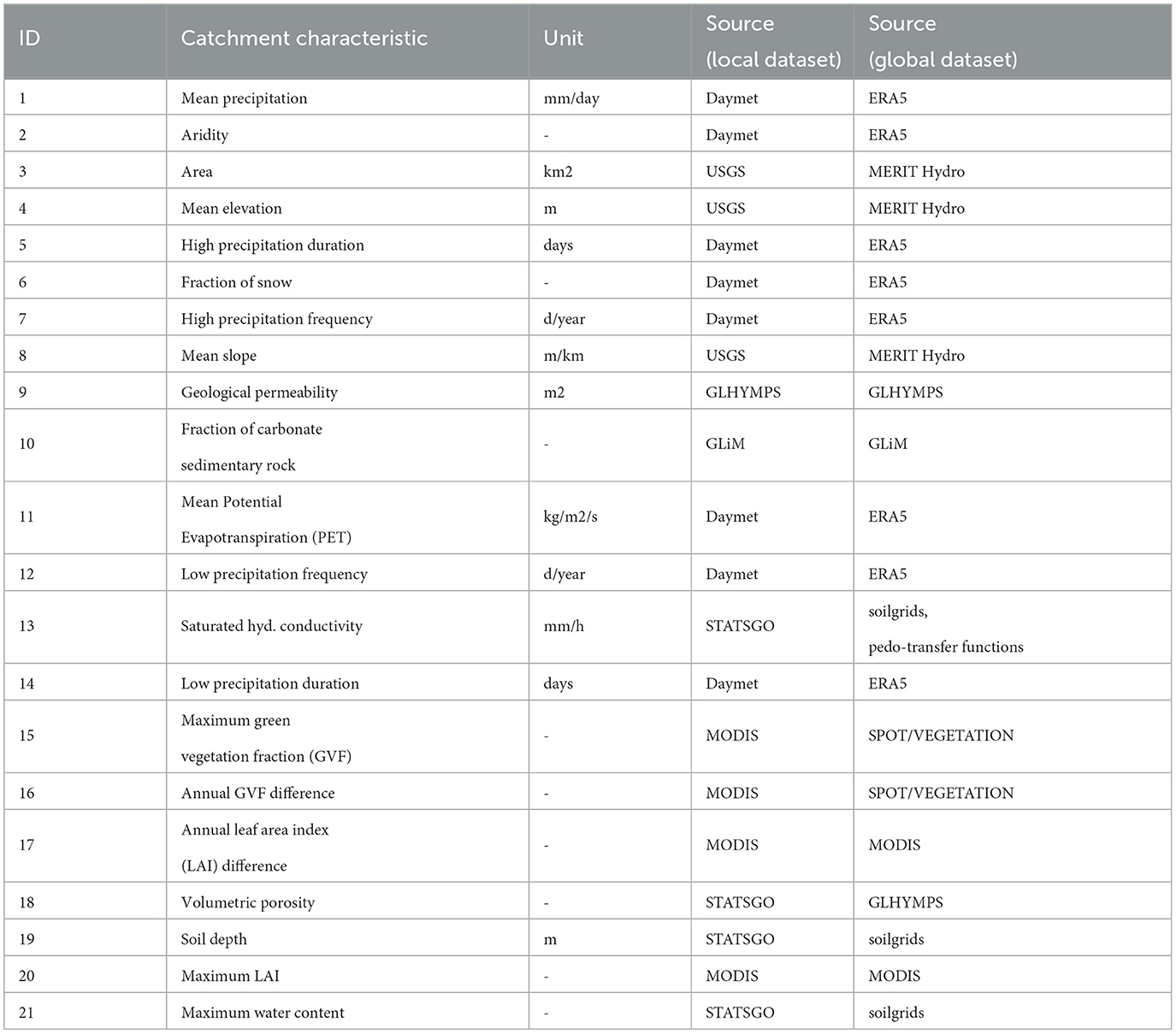
Table 2. Corresponding catchment characteristics from the local and global datasets used as static LSTM inputs, ordered by decreasing model sensitivity (Kratzert et al., 2019a).
Regardless of the employed dataset, we compute 21 static inputs from the characteristics by averaging their value over the entire catchment area and over time. Although the characteristics from local CAMELS-US and global HydroMT are broadly consistent across the chosen 516 US catchments (see Supplementary Figure S1 in the Supplementary material), some characteristics exhibit significant differences in their distributions, as shown in Figure 1. For example, the distribution of annual maximum difference in Green Vegetation (GVF; Figure 1A) is narrower for the global attribute, derived from SPOT/VEGETATION satellite data (Verger et al., 2014), compared with the local attribute, derived from the 1km land-cover product from Moderate Resolution Imaging Spectroradiometer (MODIS). Similar observations hold for the maximum water content (Figure 1B), derived globally from SoilGrids (Poggio et al., 2021) and locally from STATSGO (Miller and White, 1998). The duration of high precipitation (Gauch et al., 2021) is approximately one order of magnitude higher when the underlying meteorological data come from the local dataset compared with the global one (Figure 1C).
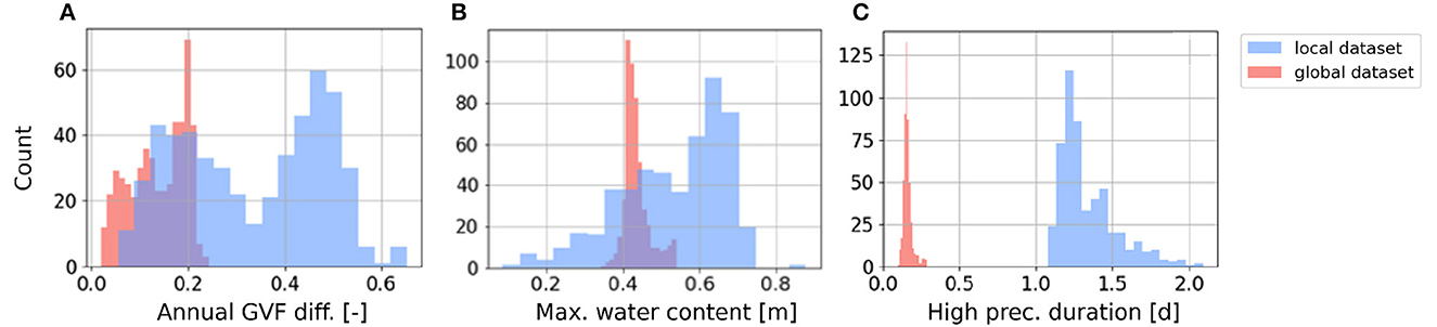
Figure 1. Distribution of static inputs for (A) annual green vegetation fraction difference, (B) maximum water content, and (C) high precipitation duration of all 516 US catchments, from local (cyan) and global (orange) datasets.
2.2. MTS-LSTM
We use the Multi-Timescale LSTM (MTS-LSTM) as implemented in NeuralHydrology (Kratzert et al., 2022a). By exploiting internal gates modeled with multi-layer perceptrons, the LSTM is able to efficiently process long time series and recognize interactions between input/output time series across lags of unknown duration. Due to this refined memory function, the LSTM can account for the meteorological conditions of the entire preceding year for predicting streamflow. LSTM-based streamflow prediction models can work with both meteorological inputs evolving over time and static inputs such as the characteristics describing the catchment conditions (Kratzert et al., 2021).
The MTS-LSTM is an architecture incorporating two LSTM that can concurrently work across different temporal resolutions using multiple branches. The MTS-LSTM employed in this study predicts streamflow at daily and hourly resolutions, using year-long historical forcing as well as hourly forcing recorded for the past 2 weeks (Gauch et al., 2021). By choosing this model for our experiments, we can test the global dataset for water management applications requiring high-frequency predictions such as flood forecasting.
The MTS-LSTM is trained to minimize a composite loss that includes the basin-averaged Nash-Sutcliffe Efficiency (NSE) (Kratzert et al., 2019b) at both daily (D) and hourly (H) time scales, as well as regularization factor to favor predictions that are consistent across timescales (Gauch et al., 2021). The regularization factor enforces consistency by penalizing solutions where daily and day-averaged hourly predictions differ significantly. The MST-LSTM loss can be written as follows:
where B represents the number of basins; is the number of samples for basin b at time scale τ; and are the observed and predicted streamflow values, respectively; σb is the observed streamflow variance of basin b over the entire training period, and ϵ is a small value to guarantee stability (Gauch et al., 2021). The first term of Eq. 1 accounts for the NSE at daily and hourly time scales, while second represents the mean squared difference regularization term based on the predictions at daily () and hourly () scales.
2.3. Clustering of catchments
To underpin the model comparison, we cluster the 516 US basins using both local and global catchment characteristic datasets, with the k-means algorithm. The comparison allows us to assess whether the global dataset describes the overall catchments in an equivalent pattern to the local one. Additionally, the models can be evaluated per catchment cluster to derive the values for combinations of characteristics that indicate good (or poor) performance. We perform the clustering following the approach of Kratzert et al. (2019b), using the analysis on the silhouette scores to identify the optimal number of clusters.
2.4. Experiments
We develop the global model by training the MTS-LSTM architecture with dynamic forcing from the global dataset ERA5 and static catchment attributes derived from global datasets via HydroMT. We test the performance of this global approach against a baseline MTS-LSTM trained using local dynamic datasets NLDAS-2 and static CAMELS-US attributes, as done in the study by Gauch et al. (2021). To separate the effects of global dynamic and global static data on model performances, we train two hybrid models where local counterparts replace either the former or the latter dataset. In total, we develop four different MTS-LSTM models with four different combinations of input data, summarized as follows:
• Global Dynamic forcing, Global Static attributes (GDGS)
• Local Dynamic forcing, Local Static attributes (LDLS)
• Global Dynamic forcing, Local Static attributes (GDLS)
• Local Dynamic forcing, Global Static attributes (LDGS)
Regardless of the above input combinations, the dynamic and static inputs fed to the LSTM models are concatenated at each time step as done in the study by Gauch et al. (2021).
2.5. Datasets and model configuration
We use data from 1980 to 2018, split into three sets as follows: a training set from 1 October 1990 to 30 September 2003, a validation set from 1 October 2003 to 30 September 2008, and a testing set from 1 October 2008 to 30 September 2018. We obtained the main set of optimal MTS-LSTM hyperparameters via grid-search for the local and global models, as shown in Table 3. We selected the remaining hyperparameters based on the study by Gauch et al. (2021).
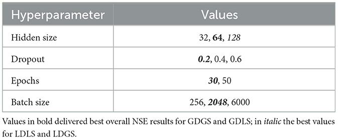
Table 3. Values tested for hyperparameter tuning of the MTS-LSTMs to obtain the best model configurations on the validation dataset, later used for testing.
2.6. Performance evaluation
All models are evaluated on the NSE, which is a widely used measure of performance for hydrologic models. For the general assessment of each model, we determine the mean NSE of all 516 US catchments and visualize a Cumulative Density Function (CDF) of the NSE values of all catchments. For flood-related applications, it is important to determine the correct timing of peaks and estimate their magnitude. To evaluate the performance regarding peak flows, we computed the bias of the high flow segment in the flow duration curve (FHV) (Yilmaz et al., 2008), the peak timing and the peak magnitude error for the daily and hourly timescales. The peak timing error is the mean of all absolute time differences between observed and modeled peak flows and determined for daily and hourly results with the same method as implemented by Gauch et al. (2021). The peak magnitude error describes the absolute and relative differences between the observed and the simulated peaks.
3. Results and discussion
3.1. Catchment clustering
The k-means algorithm (see Section 3.1) yields seven clusters for the local and eight clusters for the global dataset. The distribution of catchment clusters across the US is shown in Figure 2. Clusters show distinct geographical distribution, with global dataset clustering yielding an additional cluster for the West Coast catchments. For the remainder of the study, we will refer to the cluster numbers identified based on the global catchment dataset (clusters 1 to 8 in Figure 2B). Table 4 provides a description of each cluster, the number of catchment of each cluster, as well as the most relevant catchment characteristics, including topography, aridity, humidity, and vegetation cover. Annual and seasonal cumulative precipitation values are similar for the local and global meteorological datasets, apart from regional differences up to 20% in Western US (see Supplementary Figures S2, S3 in the Supplementary material). Higher deviations occur for daily and hourly precipitation values. The global dataset smooths out daily and hourly precipitation height and captures less small-scale rainfall events due to the coarser resolution.
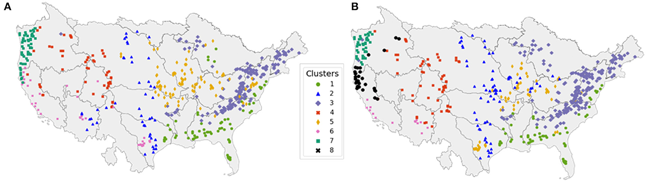
Figure 2. A total of 516 US catchments clustered based on their characteristics derived from (A) the local and (B) the global static datasets.
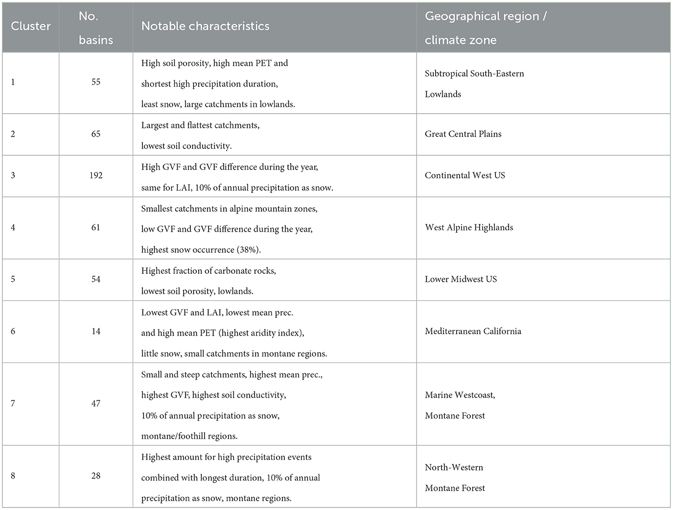
Table 4. Description of clusters build on global catchment characteristics (see map in Figure 2B).
3.2. Comparison of local, global, and hybrid MTS-LSTM models
Figure 3 reports the cumulative distribution of NSE values for all four models for daily (Figure 3A) and hourly (Figure 3B) streamflow predictions. Regardless of the timescale, the results show a performance drop for approximately 80% of the US catchments when using global dynamic forcing. These lower performances are due to the lower spatial resolution of ERA5 compared with NLDAS-2. Table 5 shows median NSE values dropping from 0.71 of the LDLS model to 0.54 for GDGS. In addition to the NSE performances, Table 5 compares median peak timing and peak height metrics of LDLS and GDGS models. The local model scores higher for all high flow metrics. The peak timing error is smaller (0.39 days vs. 0.45 days and 4.4 h vs. 4.9 h), and the magnitude of peaks is closer to the observed height model (5.77 mm/d vs. 7.75 mm/d and 0.24 mm/h vs. 0.28 mm/h). On the contrary, the model performance is not significantly different when using global compared with local catchment characteristics (LDLS vs. LDGS and GDGS vs. GDLS), which can be seen by the overlap of the cumulative density functions. This occurs for both daily and hourly streamflow predictions. Thus, the differences between local and global catchment characteristics do not influence model performance. This occurs regardless of differences in the distribution of individual characteristics (see Figure 1), as well as the omission of soil characteristics from the static model input as they are respected in the calculation of the hydraulic conductivity (see Section 2.1.3).
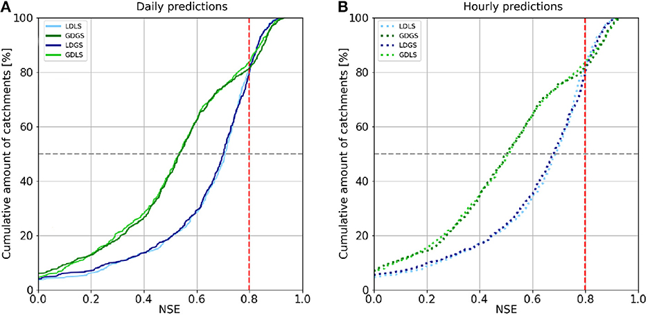
Figure 3. CDF of NSE for daily (A) and hourly results (B) of test-period for all LSTM-based models (516 catchments). The red vertical line indicates the turning point where the models trained using global dynamic forcing (GDGS and GDLS) and outperform those trained with local dynamic forcing (LDLS and LDGS). The gray horizontal lines demark accumulation of 50% of all catchments.
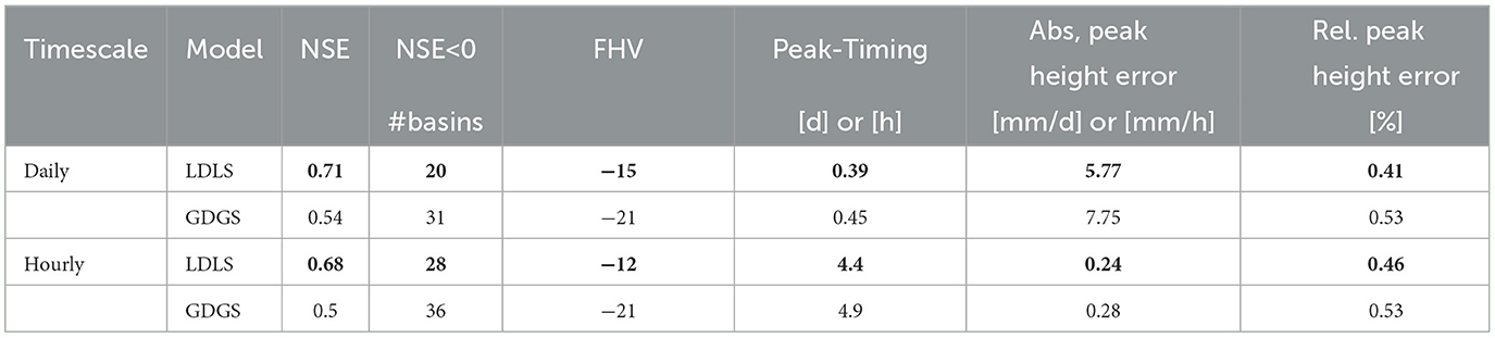
Table 5. Median metrics for local and global models. Best values per timescale in bold.
3.3. Spatial analysis of model performances
Figure 3 shows that the cumulative NSEs of both GDGS and GDLS models cross that of local models for NSE values of approximately 0.8, for both daily and hourly timescales. Figures 4, 5 provide further insights by comparing LDLS and GDGS performances spatially on the US map and individually (e.g., catchment by catchment). The spatial pattern of NSE values from LDLS resembles the distribution in the study by Gauch et al. (2021). Highest NSE values are found for the mountainous regions in the West Alpine Highlands (cluster 4), the Marine Westcoast (cluster 7), and North-Western US (cluster 8). Here, the GDGS outperforms the local models with cluster median daily NSE scores of 0.81, 0.86, and 0.84 against the lower 0.68, 0.81, and 0.80 of the LDLS (see Figure 6A). Similar results can be observed for hourly NSEs (Figure 6B), as well as for peak flow metrics such as FHV (Figures 6C, D). In the Eastern US, the LDLS performs better than the GDGS, with median daily NSEs of 0.57 vs. 0.40 for cluster 1 and 0.72 vs. 0.54 for cluster 3. Our results reflect those of the study by Tarek et al. (2020), showing a lumped conceptual hydrological model performing worse with ERA5 (our global dataset) compared with a local input dataset for the Eastern US. A main difference with respect to North-Western US is the seasonally changing vegetation cover, which subsequently demarks regions where the global dataset does not capture the meteorological conditions as precisely as the local dataset. Tarek et al. (2020) also stress that the lower performance of ERA5 in this area may result from the higher density network, favoring dynamic forcing based on observations (such as NLDAS-2). In the arid catchments of the Great Central Plains, NSE values are low for both models (cluster 2: NSE of 0.40 of LDLS vs. 0.16 of GDGS). Along with overall sparse precipitation and sudden extreme rainfall events, the long dry periods complicate the learning process for an LSTM model, and predictions of streamflow become unreliable (Gauch et al., 2021). Additionally, the global dataset misses individual small-scale rainfall events that have higher importance in very dry regions compared with humid regions.
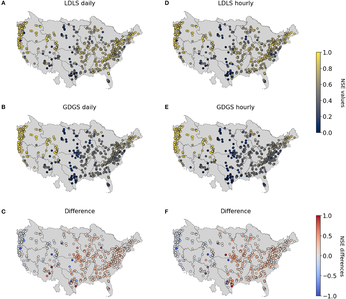
Figure 4. Spatial visualization of NSE for daily (A–C) and hourly (D–F) streamflow predictions: LDLS (A, D), GDGS (B, E), and their difference (C, F).
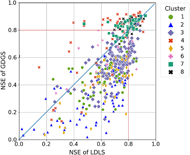
Figure 5. Comparison of individual catchment NSE values of LDLS and GDGS. Colors indicate catchment clusters (see Table 4). Catchments with negative NSE are not shown here.
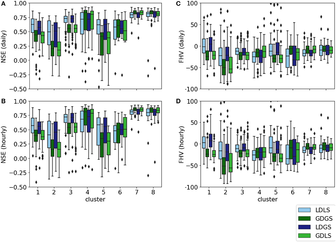
Figure 6. Boxplots of daily (A, C) and hourly (B, D) value of NSE and FHV for all catchments and models.
Overall, we observe that the global models yield highest NSE values for most catchments of Western and North-Western US (clusters 4, 6, 7, and 8), with a combined median daily NSEs of 0.83 for GDGS vs. 0.78 for LDLS. These are mainly humid, surface-runoff dominated, mountainous regions, and alpine highlands such as in North-Western US. The climatology for this region has shown largest differences between local and global precipitation compared with all other US catchments (see Section 3.1). Although local ground observations tend to underestimate precipitation in mountainous regions due to combinations of wind effects and snowfall, the local model performs worse. Additionally, satellite products, such as ERA5 global dataset used here, are known to often be too coarse to capture the thermal effects of mountains and thus misinterpret precipitation intensities (Rasmussen et al., 2012). Nevertheless, the global dataset yields better model performances in these mountainous regions. With respect to the catchment features, Figure 7 shows that GDGS performs well for catchments that are steep, with rarely occurring low precipitation, and high-saturated hydraulic conductivity. Further insights into the effects of catchment characteristics are available in Supplementary Figure S4 of the Supplementary material.
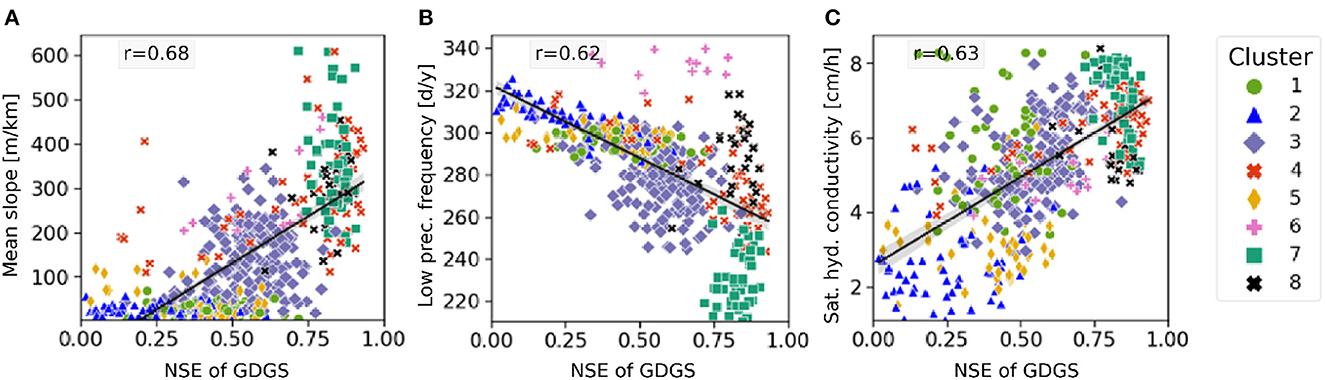
Figure 7. NSE of GDGS with respect to catchment characteristics. The results on daily timescale for catchments with NSE>0: (A) mean slope, (B) low precipitation frequency, and (C) saturated hydraulic conductivity. Colors indicate to catchment clusters. The plots also show regression line and correlation coefficient r. Plots for all 21 catchment characteristics in Supplementary Figure S1 of the Supplementary material.
4. Conclusion
To develop a hydrological DL model applicable for PUB across the globe, we require an approach that relies on meteorological time-series inputs and catchment characteristics that have identical physical meaning and identical derivation methods for all catchments worldwide. This entails working with time-series from one coherent global dataset, as well as catchment characteristics derived from global datasets. In this study, we performed a preliminary assessment on the suitability of a global MTS-LSTM model trained with global dynamic forcing datasets ERA5 and global static catchment characteristics retrieved by HydroMT (GDGS). We compared this global model with an MTS-LSTM trained on local datasets (LDLS) with state-of-the-art performances (Gauch et al., 2021). On average, our results show that the global model underperforms the local one. Nevertheless, the global model clearly outperforms the local model for catchments in Western and North-Western US, especially for NSE>0.8.
Our extensive analysis including hybrid models GDLS and LDGS showed that changing the source dataset for the catchment characteristics from local to global did not affect the model performance significantly. We, therefore, suggest that an in-depth research on the choice of relevant catchment characteristics can be beneficial to clarify the influence of different types of characteristics as follows: a) those derived from the meteorological forcing like mean precipitation and PET; b) those redundantly represented like the soil composition in the saturated hydraulic conductivity; or c) those with extremely different distributions when derived from different datasets such as the GVF from MODIS vs. SPOT/VEGETATION. The performance differences between the local and global models originate from the meteorological inputs. We observed the global model outperforming for surface-runoff dominated catchments in humid climate and mountainous regions.
Based on our catchment clustering, catchments with matching characteristics can be identified worldwide. The next step is, then, to test how well the global model performs in gauged catchments outside of the US, similar to those high-performing clusters. These should be treated as ungauged (i.e., pretending no streamflow observations exist) and compared with other models suitable for PUB.
Furthermore, we expect to obtain a more powerful global model, with higher general validity when including data from other continents in the training. This is particularly true for the prediction of extreme events, which requires including high return period events in the training to achieve better extrapolation (Frame et al., 2022). We can identify a higher number of gauged catchments exposed to extreme events by widening the geographical coverage.
The global forcing dataset results in a performance drop for catchments in the Eastern US, probably caused by dampened representation of seasonality in the meteorological forcing (Tarek et al., 2020). Therefore, for future studies, we suggest testing other meteorological datasets [or combination of them, see Kratzert et al. (2021)], with hourly temporal resolution as input for a global model. The alternative datasets should be of higher spatial resolution than ERA5, as most catchments included in our study had an area smaller than a grid-cell of the global dataset (31x31km). One option is the MSWEP dataset with an 11x11km grid, identified as the best openly accessible global precipitation dataset (Beck et al., 2019).
Another promising global forcing dataset is the EM-Earth dataset, recently published by Tang et al. (2022) and based on in-situ observations combined with ERA5 data. The advantages of ERA5 are the back-extension until 1950 and the upcoming release of future scenarios, which could potentially be transferred to the EM-Earth dataset and enable extensive studies on climate effects over multiple decades. However, another option is provided by the newly released Caravan global community dataset (Kratzert et al., 2022b), which is designed to facilitate the development of global models. Caravan consists of global dynamic forcing based on ERA5 Land, catchment characteristics based on HydroATLAS, and streamflow data from multiple regional discharge datasets.
Regardless of the chosen global forcing dataset, it is crucial to acknowledge that their dependability differs across various regions of the world. Consequently, additional efforts are required to validate streamflow predictions derived from global input time series. However, we expect significant future improvements in the reliability of global datasets, mainly due to increased satellite density and advanced data merging algorithms, which combine a diverse range of sources including Low-Earth Orbit and Geosynchronous Equatorial Orbit satellites, numerical weather prediction models, and in-situ observations (Sun et al., 2018).
Data availability statement
We used the NeuralHydrology Python Library for all our experiments, available at https://neuralhydrology.github.io/. Streamflow data and local datasets available from Gauch et al. (2021). Global forcing data available from Hersbach et al. (2020). The HydroMT software used to extract global static features is available at https://github.com/Deltares/hydromt.
Author contributions
KW: conceptualization, methodology, validation, software, writing—original draft, and visualization. RT: conceptualization, methodology, validation, writing—original draft, writing—review and editing, visualization, supervision, project administration, and resources. M-CtV, JN, and MH: conceptualization and writing—review and editing. MV: conceptualization, writing—review and editing, and supervision. RD: conceptualization, writing—review and editing, supervision, project administration, and resources. All authors contributed to the article and approved the submitted version.
Acknowledgments
This manuscript is based on the Master of Science thesis of Wilbrand (2021). The authors are grateful to the reviewers for their constructive feedback and insightful suggestions.
Conflict of interest
The authors declare that the research was conducted in the absence of any commercial or financial relationships that could be construed as a potential conflict of interest.
Publisher's note
All claims expressed in this article are solely those of the authors and do not necessarily represent those of their affiliated organizations, or those of the publisher, the editors and the reviewers. Any product that may be evaluated in this article, or claim that may be made by its manufacturer, is not guaranteed or endorsed by the publisher.
Supplementary material
The Supplementary Material for this article can be found online at: https://www.frontiersin.org/articles/10.3389/frwa.2023.1166124/full#supplementary-material
References
Addor, N., Newman, A. J., Mizukami, N., and Clark, M. P. (2017). The camels data set: catchment attributes and meteorology for large-sample studies. Hydrol. Earth Syst. Sci. 21, 5293–5313. doi: 10.5194/hess-21-5293-2017
Arsenault, R., Martel, J.-L., Brunet, F., Brissette, F., and Mai, J. (2023). Continuous streamflow prediction in ungauged basins: long short-term memory neural networks clearly outperform traditional hydrological models. Hydrol. Earth Syst. Sci. 27, 139–157. doi: 10.5194/hess-27-139-2023
Ayzel, G., Kurochkina, L., Kazakov, E., and Zhuravlev, S. (2020). “Streamflow prediction in ungauged basins: benchmarking the efficiency of deep learning,” in E3S Web of Conferences. Les Ulis, France: EDP Sciences. doi: 10.1051/e3sconf/202016301001
Beck, H. E., Wood, E. F., Pan, M., Fisher, C. K., Miralles, D. G., Van Dijk, A. I., et al. (2019). Mswep v2 global 3-hourly 0.1 precipitation: methodology and quantitative assessment. Bull. Am. Meteorol. Soc. 100, 473–500. doi: 10.1175/BAMS-D-17-0138.1
Bouaziz, L. J., Fenicia, F., Thirel, G., de Boer-Euser, T., Buitink, J., Brauer, C. C., et al. (2021). Behind the scenes of streamflow model performance. Hydrol. Earth Syst. Sci. 25, 1069–1095. doi: 10.5194/hess-25-1069-2021
Cosby, B., Hornberger, G., Clapp, R., and Ginn, T. (1984). A statistical exploration of the relationships of soil moisture characteristics to the physical properties of soils. Water Resour. Res. 20, 682–690. doi: 10.1029/WR020i006p00682
Eilander, D., Boisgontier, H., Bouaziz, L. J. E., Buitink, J., Couasnon, A., Dalmijn, B., et al. (2023). HydroMT: Automated and reproducible model building and analysis. J. Open Source Softw. 8, 4897.
Fang, K., Kifer, D., Lawson, K., Feng, D., and Shen, C. (2022). The data synergy effects of time-series deep learning models in hydrology. Water Resour. Res. 58, e2021WR029583. doi: 10.1029/2021WR029583
Fang, K., Kifer, D., Lawson, K., and Shen, C. (2020). Evaluating the potential and challenges of an uncertainty quantification method for long short-term memory models for soil moisture predictions. Water Resour. Res. 56, e2020WR028095. doi: 10.1029/2020WR028095
Frame, J. M., Kratzert, F., Klotz, D., Gauch, M., Shelev, G., Gilon, O., et al. (2022). Deep learning rainfall-runoff predictions of extreme events. Hydrol. Earth Syst. Sci. 26, 3377–3392. doi: 10.5194/hess-26-3377-2022
Gao, H., Hrachowitz, M., Sriwongsitanon, N., Fenicia, F., Gharari, S., and Savenije, H. H. (2016). Accounting for the influence of vegetation and landscape improves model transferability in a tropical savannah region. Water Resour. Res. 52, 7999–8022. doi: 10.1002/2016WR019574
Gauch, M., Kratzert, F., Klotz, D., Nearing, G., Lin, J., and Hochreiter, S. (2021). Rainfall-runoff prediction at multiple timescales with a single long short-term memory network. Hydrol. Earth Syst. Sci. 25, 2045–2062. doi: 10.5194/hess-25-2045-2021
Gharari, S., Gupta, H. V., Clark, M. P., Hrachowitz, M., Fenicia, F., Matgen, P., et al. (2021). Understanding the information content in the hierarchy of model development decisions: Learning from data. Water Resour. Res. 57, e2020WR027948. doi: 10.1029/2020WR027948
Götzinger, J., and Bárdossy, A. (2007). Comparison of four regionalisation methods for a distributed hydrological model. J. Hydrol. 333:374–384. doi: 10.1016/j.jhydrol.2006.09.008
Hersbach, H., Bell, B., Berrisford, P., Hirahara, S., Horányi, A., Mu noz-Sabater, J., et al. (2020). The era5 global reanalysis. Q. J. R. Meteorol. Soc. 146, 1999–2049. doi: 10.1002/qj.3803
Hochreiter, S., and Schmidhuber, J. (1997). Long short-term memory. Neural Comput. 9, 1735–1780. doi: 10.1162/neco.1997.9.8.1735
Hrachowitz, M., Savenije, H., Blöschl, G., McDonnell, J., Sivapalan, M., Pomeroy, J., et al. (2013). A decade of predictions in ungauged basins (pub)–a review. Hydrol. Sci. J. 58, 1198–1255. doi: 10.1080/02626667.2013.803183
Imhoff, R., Van Verseveld, W., Van Osnabrugge, B., and Weerts, A. (2020). Scaling point-scale (pedo) transfer functions to seamless large-domain parameter estimates for high-resolution distributed hydrologic modeling: An example for the rhine river. Water Resour. Res. 56, e2019WR026807. doi: 10.1029/2019WR026807
Kratzert, F., Gauch, M., Nearing, G., and Klotz, D. (2022a). Neuralhydrology–a python library for deep learning research in hydrology. J. Open Source Software. 7, 4050. doi: 10.21105/joss.04050
Kratzert, F., Klotz, D., Brenner, C., Schulz, K., and Herrnegger, M. (2018). Rainfall-runoff modelling using long short-term memory (lstm) networks. Hydrol. Earth Syst. Sci. 22, 6005–6022. doi: 10.5194/hess-22-6005-2018
Kratzert, F., Klotz, D., Herrnegger, M., Sampson, A. K., Hochreiter, S., and Nearing, G. S. (2019a). Toward improved predictions in ungauged basins: Exploiting the power of machine learning. Water Resour. Res. 55, 11344–11354. doi: 10.1029/2019WR026065
Kratzert, F., Klotz, D., Hochreiter, S., and Nearing, G. S. (2021). A note on leveraging synergy in multiple meteorological data sets with deep learning for rainfall-runoff modeling. Hydrol. Earth Syst. Sci. 25, 2685–2703. doi: 10.5194/hess-25-2685-2021
Kratzert, F., Klotz, D., Shalev, G., Klambauer, G., Hochreiter, S., and Nearing, G. (2019b). Towards learning universal, regional, and local hydrological behaviors via machine learning applied to large-sample datasets. Hydrol. Earth Syst. Sci. 23, 5089–5110. doi: 10.5194/hess-23-5089-2019
Kratzert, F., Nearing, G., Addor, N., Erickson, T., Gauch, M., Gilon, O., et al. (2022b). Caravan-a global community dataset for large-sample hydrology. Scientific Data. 10, 61. doi: 10.31223/X50S70
Kumar, R., Samaniego, L., and Attinger, S. (2013). Implications of distributed hydrologic model parameterization on water fluxes at multiple scales and locations. Water Resour. Res. 49:360–379. doi: 10.1029/2012WR012195
Lees, T., Buechel, M., Anderson, B., Slater, L., Reece, S., Coxon, G., et al. (2021). Benchmarking data-driven rainfall-runoff models in great britain: a comparison of long short-term memory (lstm)-based models with four lumped conceptual models. Hydrol. Earth Syst. Sci. 25, 5517–5534. doi: 10.5194/hess-25-5517-2021
Ma, K., Feng, D., Lawson, K., Tsai, W.-P., Liang, C., Huang, X., et al. (2021). Transferring hydrologic data across continents-leveraging data-rich regions to improve hydrologic prediction in data-sparse regions. Water Resour. Res. 57, e2020WR028600. doi: 10.1029/2020WR028600
Mai, J., Shen, H., Tolson, B. A., Gaborit, É., Arsenault, R., Craig, J. R., et al. (2022). The great lakes runoff intercomparison project phase 4: the great lakes (grip-gl). Hydrol. Earth Syst. Sci. 26:3537–3572. doi: 10.5194/hess-26-3537-2022
Merz, R., and Blöschl, G. (2004). Regionalisation of catchment model parameters. J. Hydrol. 287, 95–123. doi: 10.1016/j.jhydrol.2003.09.028
Miller, D. A., and White, R. A. (1998). A conterminous united states multilayer soil characteristics dataset for regional climate and hydrology modeling. Earth Interact. 2, 1–26. doi: 10.1175/1087-3562(1998)002<0001:ACUSMS>2.3.CO;2
Oreshkin, B. N., Carpov, D., Chapados, N., and Bengio, Y. (2021). Meta-learning framework with applications to zero-shot time-series forecasting. Proc. Innov. Appl. Artif. Intell. Conf. 35, 9242–9250. doi: 10.1609/aaai.v35i10.17115
Poggio, L., De Sousa, L. M., Batjes, N. H., Heuvelink, G., Kempen, B., Ribeiro, E., et al. (2021). Soilgrids 2.0: producing soil information for the globe with quantified spatial uncertainty. Soil 7:217–240. doi: 10.5194/soil-7-217-2021
Rasmussen, R., Baker, B., Kochendorfer, J., Meyers, T., Landolt, S., Fischer, A. P., et al. (2012). How well are we measuring snow: The noaa/faa/ncar winter precipitation test bed. Bull. Am. Meteorol. Soc. 93:811–829. doi: 10.1175/BAMS-D-11-00052.1
Samaniego, L., Kumar, R., and Attinger, S. (2010). Multiscale parameter regionalization of a grid-based hydrologic model at the mesoscale. Water Resour. Res. 46, 5. doi: 10.1029/2008WR007327
Shen, C. (2018). A transdisciplinary review of deep learning research and its relevance for water resources scientists. Water Resour. Res. 54, 8558–8593. doi: 10.1029/2018WR022643
Sivapalan, M., Takeuchi, K., Franks, S., Gupta, V., Karambiri, H., Lakshmi, V., et al. (2003). Iahs decade on predictions in ungauged basins (pub), 2003-2012: Shaping an exciting future for the hydrological sciences. Hydrological Sci. J. 48, 857–880. doi: 10.1623/hysj.48.6.857.51421
Sun, Q., Miao, C., Duan, Q., Ashouri, H., Sorooshian, S., and Hsu, K.-L. (2018). A review of global precipitation data sets: data sources, estimation, and intercomparisons. Rev. Geophys. 56, 79–107. doi: 10.1002/2017RG000574
Tang, G., Clark, M. P., and Papalexiou, S. M. (2022). Em-earth: the ensemble meteorological dataset for planet earth. Bull. Am. Meteorol. Soc. 103, E996–E1018. doi: 10.1175/BAMS-D-21-0106.1
Tarek, M., Brissette, F. P., and Arsenault, R. (2020). Evaluation of the era5 reanalysis as a potential reference dataset for hydrological modelling over north america. Hydrol. Earth Syst. Sci. 24, 2527–2544. doi: 10.5194/hess-24-2527-2020
Verger, A., Baret, F., and Weiss, M. (2014). Near real-time vegetation monitoring at global scale. IEEE J. Sel. Top. Appl. Earth Obs. Remote Sens. 7, 3473–3481. doi: 10.1109/JSTARS.2014.2328632
Wilbrand, K. (2021). Assessing Global Applicability of a Long Short-Term Memory (lstm) Neural Network for Rainfall-Runoff Modelling. Available online at: http://resolver.tudelft.nl/uuid:90bcda06-c835-4670-bb13-1f793b4c7763
Xia, Y., Mitchell, K., Ek, M., Sheffield, J., Cosgrove, B., Wood, E., et al. (2012). Continental-scale water and energy flux analysis and validation for the north american land data assimilation system project phase 2 (nldas-2): 1. intercomparison and application of model products. J. Geophys. Res. 117, D3. doi: 10.1029/2011JD016048
Yilmaz, K. K., Gupta, H. V., and Wagener, T. (2008). A process-based diagnostic approach to model evaluation: application to the nws distributed hydrologic model. Water Resour. Res. 44(9). doi: 10.1029/2007WR006716
Keywords: rainfall-runoff modeling, LSTM, deep learning, global datasets, ERA5, streamflow prediction
Citation: Wilbrand K, Taormina R, ten Veldhuis M-C, Visser M, Hrachowitz M, Nuttall J and Dahm R (2023) Predicting streamflow with LSTM networks using global datasets. Front. Water 5:1166124. doi: 10.3389/frwa.2023.1166124
Received: 14 February 2023; Accepted: 05 May 2023;
Published: 05 June 2023.
Edited by:
Quoc Bao Pham, University of Silesia in Katowice, PolandReviewed by:
Hristos Tyralis, Hellenic Air Force, GreeceMatteo Sangiorgio, Polytechnic University of Milan, Italy
K. S. Kasiviswanathan, Indian Institute of Technology Roorkee, India
Copyright © 2023 Wilbrand, Taormina, ten Veldhuis, Visser, Hrachowitz, Nuttall and Dahm. This is an open-access article distributed under the terms of the Creative Commons Attribution License (CC BY). The use, distribution or reproduction in other forums is permitted, provided the original author(s) and the copyright owner(s) are credited and that the original publication in this journal is cited, in accordance with accepted academic practice. No use, distribution or reproduction is permitted which does not comply with these terms.
*Correspondence: Riccardo Taormina, ci50YW9ybWluYUB0dWRlbGZ0Lm5s
†These authors have contributed equally to this work