 Jacob A. Zwart1*
 Jeremy Diaz1
 Scott Hamshaw1
 Samantha Oliver2Jesse C. Ross1Margaux Sleckman1
 Alison P. Appling1Hayley Corson-Dosch1
 Xiaowei Jia3Jordan Read1,4Jeffrey Sadler1,5Theodore Thompson1David Watkins1Elaheh White1
- 1U.S. Geological Survey, Water Mission Area, Reston, VA, United States
- 2U.S. Geological Survey, Upper Midwest Water Science Center, Madison, WI, United States
- 3Department of Computer Science, University of Pittsburgh, Pittsburgh, PA, United States
- 4Consortium of Universities for the Advancement of Hydrologic Science, Inc., Arlington, MA, United States
- 5Biosystems & Agricultural Engineering, Oklahoma State University, Stillwater, OK, United States
Deep learning (DL) models are increasingly used to forecast water quality variables for use in decision making. Ingesting recent observations of the forecasted variable has been shown to greatly increase model performance at monitored locations; however, observations are not collected at all locations, and methods are not yet well developed for DL models for optimally ingesting recent observations from other sites to inform focal sites. In this paper, we evaluate two different DL model structures, a long short-term memory neural network (LSTM) and a recurrent graph convolutional neural network (RGCN), both with and without data assimilation for forecasting daily maximum stream temperature 7 days into the future at monitored and unmonitored locations in a 70-segment stream network. All our DL models performed well when forecasting stream temperature as the root mean squared error (RMSE) across all models ranged from 2.03 to 2.11°C for 1-day lead times in the validation period, with substantially better performance at gaged locations (RMSE = 1.45–1.52°C) compared to ungaged locations (RMSE = 3.18–3.27°C). Forecast uncertainty characterization was near-perfect for gaged locations but all DL models were overconfident (i.e., uncertainty bounds too narrow) for ungaged locations. Our results show that the RGCN with data assimilation performed best for ungaged locations and especially at higher temperatures (>18°C) which is important for management decisions in our study location. This indicates that the networked model structure and data assimilation techniques may help borrow information from nearby monitored sites to improve forecasts at unmonitored locations. Results from this study can help guide DL modeling decisions when forecasting other important environmental variables.
Introduction
Near-term environmental forecasts aid water resource managers in meeting both human and ecological needs. For example, forecasts of lake water quality enable better informed decisions about in situ management to meet safe drinking water criteria (Thomas et al., 2020), broad-scale flood forecasts alert the public and emergency responders to potentially harmful water inundation (Nevo et al., 2022), and forecasts of the distribution of endangered aquatic species (e.g., Atlantic sturgeon [Acipenser oxyrinchus]) allow commercial fishers to steer clear of potentially harmful interactions (Breece et al., 2021). Similarly, managers can use water temperature forecasts and monitoring to mitigate fish stress during warm periods through short-term interventions such as temporary fishing restrictions and closures (Boyd et al., 2010; Gale et al., 2013; Jeanson et al., 2021) or timed cool-water releases from reservoirs (Jager and Smith, 2008; Olden and Naiman, 2010; Zwart et al., 2022). Aquatic forecasts are important tools for managing water resources, and there are benefits to aquatic science and society when advances in environmental modeling techniques are applied to forecasting problems (Dietze et al., 2018).
Recent advances in data-driven, deep learning (DL) models show improvements for aquatic forecasting (Nearing et al., 2021b; Appling et al., 2022; Varadharajan et al., 2022; Zwart et al., 2022). DL models learn complex environmental relationships and can be extremely accurate when predicting under a variety of conditions and locations with sufficient training data (e.g., Read et al., 2019; Fang and Shen, 2020; Feng et al., 2020). For example, DL models have outperformed process-based and statistical alternatives for stream temperature predictions with respect to Nash Sutcliffe Efficiency (NSE) and bias (Rahmani et al., 2020) and have yielded similar or better root mean square errors (RMSEs) for stream dissolved oxygen predictions across the continental United States compared to regional non-DL models with more input data (Zhi et al., 2021). Once trained, DL models have trivial time costs for prediction, meaning that forecasts can be delivered nearly as quickly as the forcing data, allowing for quick management decisions. A growing number of examples of DL models are being used for water forecasting applications, including for streamflow (Feng et al., 2020; Xiang and Demir, 2020; Nevo et al., 2022), harmful algal blooms (Kim et al., 2022), water demand (Guo et al., 2018), and stream temperature (Zwart et al., 2022). DL models with temporal awareness, such as a long-short term memory network (LSTM), are designed to learn and remember long-term dependencies in sequential data, making them particularly wellsuited for environmental time series forecasting. Spatial variants of LSTMs, such as a recurrent graph convolutional neural network (RGCN), also known as GCN-LSTM (Sun et al., 2021), extend the capabilities of LSTMs by incorporating graph-based structures to model complex spatial relationships, and are particularly effective in applications that involve spatially distributed data with meaningful connections, such as stream networks (Jia et al., 2021). Techniques that introduce process guidance, such as adding in custom loss functions penalizing the model when it violates physical laws (Read et al., 2019), pretraining the DL model on process-based model output (Jia et al., 2021), and adding in structural awareness of real-world systems (Daw et al., 2020; Karniadakis et al., 2021) have shown to improve DL model prediction accuracy, especially when making predictions in locations or time periods that are outside the training dataset (Willard et al., 2022). DL models can also make use of real-time observations by ingesting these data via autoregressive techniques (Nearing et al., 2021a), data integration kernels (Fang and Shen, 2020), ensemble-based data assimilation methods (Zwart et al., 2022), or inverse neural network-based methods (Chen et al., 2021). Ingesting recent observations into DL models can help correct for errors in the models in real-time and potentially make use of nearby observations for unmonitored locations. These technical advances in DL modeling show improvements for forecasting many aquatic variables and aid in decision making.
Forecasting aquatic variables becomes much more challenging in unmonitored locations because general relationships and information learned at monitored locations would need to be appropriately applied to the unmonitored locations (Hrachowitz et al., 2013; Meyer and Pebesma, 2021). This prediction challenge has spurred decades of research in the hydrologic community to develop techniques to improve predictions at unmonitored locations with progress in monitoring networks, hydrologic theory, statistical methods, and process-based modeling (Sivapalan et al., 2003; Hrachowitz et al., 2013). However, DL techniques have recently been shown to have superior performance at predicting water quantity and quality in unmonitored locations even over the state-of-the-art process-based models; for example, LSTMs of lake temperature that are trained on wellmonitored lakes and transferred to unmonitored lakes yield lower RMSEs than a process-based modeling alternative 1.88 vs. 2.34°C (Willard et al., 2021); median NSE was higher for an LSTM predicting in out-of-sample basins (0.69) than for a calibrated Sacramento Soil Moisture Accounting (SAC-SMA) model (0.64) or the National Water Model (0.58) (Kratzert et al., 2019); and streamflow Kling-Gupta Efficiencies (KGEs) were 0.556 for a DL model applied to out-of-sample regions (harder) and 0.46 for the process-based HBV model applied to out-of-sample basins (easier yet worse KGE) (Feng et al., 2021). DL models and their process-guided variants are currently the best tools for extrapolation to unmonitored locations, such that evaluation of current architectures and further improvement to these models is likely to advance our overall forecasting capability.
In this paper, we evaluate two different DL model architectures, LSTM and RGCN, both with and without data assimilation (DA) for forecasting daily maximum stream water temperature 7 days into the future at monitored and unmonitored locations in the upper Delaware River Basin in the northeastern United States; this is a natural extension of the previous analysis described in Zwart et al. (2022) where they forecasted stream temperature only at monitored locations within the DRB. We conducted a k-fold spatial cross-validation experiment where we withheld representative river segments for each fold and validated each model on these “unmonitored” locations during a validation period where we issued 7-day forecasts for 354 consecutive forecast issue days. Based on the validation results, we chose a model with which to issue 7-day forecasts for 522 consecutive forecast issue days in a separate test period. The best performing model from this experiment can be trained on all available data in the stream network and used to make operational forecasts of maximum water temperature in the Delaware River Basin. These operational forecasts can aid water resources managers in optimizing reservoir releases to cool downstream river segments while retaining enough water to supply New York City and other municipalities with drinking water.
Methods
Study site
Our objective was to generate accurate forecasts of daily maximum stream water temperature (hereafter referred to as “maximum water temperature”) at 70 locations (both monitored and unmonitored) in the upper Delaware River Basin in support of drinking water reservoir management decisions (Figure 1). The Delaware River Basin is an ecologically diverse region and a societally important watershed along the East Coast of the United States as it provides drinking water to more than 15 million people (Williamson and Lant, 2015). A multi-state agreement includes provisions that aim to maintain maximum water temperature below 23.89°C (75°F) in the upper Delaware River Basin upstream from Lordville, New York, to ensure cold-water stream habitat. The Neversink watershed in northeastern Delaware River Basin is home to similarly temperature-sensitive populations of recreationally and environmentally important species such as brook trout (Salvelinus fontinalis), brown trout (Salmo trutta), and dwarf wedgemussel (Alasmidonta heterodon) (Lawrence et al., 2001; St. John White et al., 2017). Forecasts of stream water temperature can be used to anticipate expected exceedances of the 23.89°C thermal threshold and help managers with decisions on deep, cool water releases from reservoirs to mitigate temperature exceedances. For more details on the Delaware River Basin study location, see (Zwart et al., 2022).
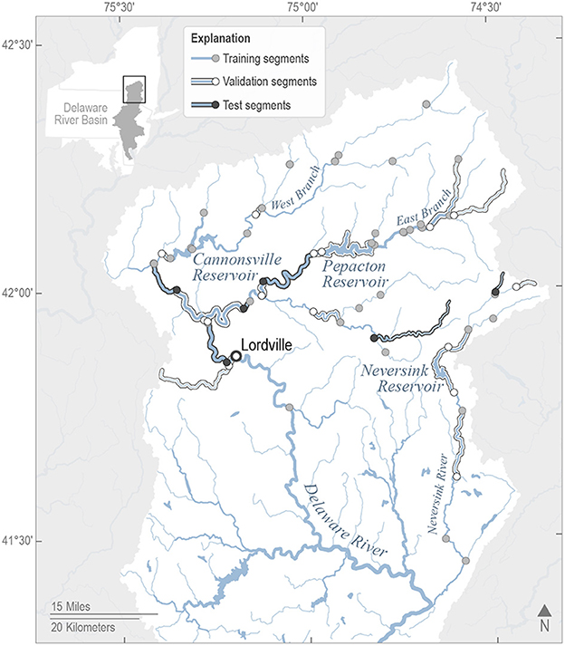
Figure 1. Map of the target water temperature forecasting sites in the upper Delaware River Basin as indicated by training, validation, and test stream segments along the stream network. The stream segments' downstream endpoints were our forecast target sites and are indicated by circles on the map. Training segments are indicated by a gray circle and a blue upstream segment, validation segments are indicated by a white circle and white highlighted upstream segment, and test segments are indicated by a black circle and black highlighted upstream segment. The Delaware River at Lordville site is indicated with a bolded open circle where management provisions aim to maintain maximum water temperature below 23.89°C (75°F).
Datasets and model development overview
We used 5-fold spatial cross-validation to train our models and assessed their performance on a spatial validation set. We then selected the best model from this evaluation and tested it on a representative holdout set of sites. Each cross-validation fold omitted the same 6 testing sites and 3–4 strategically selected wellobserved validation sites (Figure 1). The 6 testing sites contained 2 mainstem stream segments, 2 headwater stream segments, and 2 reservoir-impacted stream segments, and the validation sets for each fold contained at least 1 of each of the mainstem, headwater, and reservoir-impacted stream segments. Reservoir-impacted stream segments were segments directly downstream from the New York City drinking water reservoirs or within 3 stream segments of the reservoirs. Mainstem stream segments were those on the East or West Branch of the Delaware River and the Neversink River that were 4th order streams or greater, while the rest of the segments were considered headwater stream segments. The testing and validation sites were used to simulate unmonitored (hereafter named “ungagged”) conditions. Our aim was to assess the model's performance on both gaged and ungaged segments while encountering previously unobserved conditions. Thus, we used the 2019 calendar year as our validation time period for all 5 spatial cross-validation folds and April 2021 to September 2022 as our testing time period and withheld these times during training. First, we pretrained our stream network DL models on process-based model output to guide the model toward more physically consistent predictions of water temperature as in Jia et al. (2021) and Zwart et al. (2022), but see Topp et al. (2023) for limitations to this approach. Next, we fine-tuned our models on observed maximum daily water temperatures. Using the trained models, we then forecasted maximum water temperature 7 days into the future for every issue date (forecasts issued daily) during the validation period. Finally, we adopted the model framework (i.e., architecture and choice of DA or not) that performed best across spatial cross-validation experiments, re-trained this model on all available training data (including 2019 validation year and all non-test sites), and issued daily forecasts in the testing period. Below, we describe the pretraining, fine-tuning, and forecasting datasets used to make near-term forecasts of water temperature.
Spatial fabric
We used the National Geospatial Fabric to define the physical characteristics (stream segment length, slope, and elevation) of 70 stream reaches (Figure 1), each with <1 day travel time, whose downstream endpoints were our 70 target sites (Viger, 2014; Viger and Bock, 2014).
Stream temperature observation dataset
We downloaded sub-daily observations of stream water temperature from U.S. Geological Survey's (USGS) National Water Information System (NWIS) (US Geological Survey, 1994; date accessed: 2022-03-23), the Water Quality Portal (WQP; Read et al., 2017; date accessed: 2022-03-23), and Spatial Hydro-Ecological Decision System (EcoSHEDS, http://db.ecosheds.org/; date accessed: 2022-03-23). We assigned and aggregated these observations to stream reaches and daily maxima as described in Zwart et al. (2022) for both the fine-tuning dataset and for assimilating when making forecasts.
Historical driver dataset
We used 10 dynamic drivers (i.e., input features) to train our DL models from 1982 to 2020 (excluding the 2019 validation year), including gridMET daily minimum air temperature and relative humidity, daily mean downward shortwave radiation, wind speed, and relative humidity, daily maximum air temperature and relative humidity, and daily accumulated precipitation (Abatzoglou, 2013). As additional dynamic input features, we also used NWIS daily mean reservoir release rate at reservoir gage locations, and observations of yesterday's maximum water temperature. Reservoir releases were applied only to sites where the reservoirs were discharging water (3 stream segments), while all other sites this input was set to zero for all times (67 stream segments). When observations of yesterday's maximum water temperature were not available, we used yesterday's predicted daily mean water temperature from the process model pretraining dataset (described below). We also used four static input features to train our models including stream reach mean elevation, slope, length, and mean stream width. These static features did not change with time for each segment and were also used in the forecast driver dataset (see description below).
Process-based model pretraining dataset
We used process-based model output from 1982 to 2020 (excluding the 2019 validation year) to pretrain the DL models before fine-tuning on observations of maximum water temperature. In-depth details on the pretraining dataset can be found in Zwart et al. (2022), and we briefly describe this dataset here. We used the Precipitation Runoff Modeling System with a coupled Stream Temperature Network model (PRMS-SNTemp) to make initial predictions of daily mean stream temperature (Markstrom, 2012; Sanders et al., 2017) using the calibrated flow parameters of Regan et al. (2018). Following Zwart et al. (2022), we simulated the water temperature of reservoir releases from two major reservoirs in the basin, Cannonsville and Pepacton Reservoirs, using the General Lake Model (GLM v3.1; Hipsey et al., 2019). We combined outputs from these two models by computing a weighted mean of temperature predictions from PRMS-SNTemp and GLM, where GLM predictions only affected stream segments downstream from GLM-simulated reservoirs. The weight given to GLM predictions was a function of distance downstream from the reservoir, where segments closer to the upstream reservoirs had stream water temperatures more similar to the output from GLM.
Forecasted driver dataset
During the 2019 validation period, we generated forecasts using the National Oceanic and Atmospheric Administration's Global Ensemble Forecast System model version 12.0 0.25-degree reforecast archive (GEFS, https://noaa-gefs-retrospective.s3.amazonaws.com/index.html), and we used the operational GEFSv12 0.25-degree archive during the testing period (https://registry.opendata.aws/noaa-gefs/). The GEFS reforecast archive spans 2000–2019 and we used a GEFS operational archive for 2021–2022 for testing. For both GEFS datasets, we aggregated the GEFSv12 sub-daily output of the day-0 forecasts to daily meteorological drivers that matched the gridMET drivers used in the training phase. The GEFS reforecast and operational archive contains the 00 UTC (19:00 EDT) forecast cycle for each day, and saves valid times at 3-hour intervals (i.e., 00:00, 03:00, etc.) in UTC for 240 hours past the forecast issue time. Starting with the 03:00 valid time, values at each timestep represent the mean, minimum, or maximum of the preceding 3 hours depending on the meteorological driver forecasted. To transform these 3-hourly values to daily values in mean solar time in the Delaware River Basin (approximately UTC −5:00), we treated the 09:00 through 30:00 UTC (4:00–25:00 in UTC −5:00) timesteps as day 0. This provided the closest possible alignment of GEFS timesteps with mean solar time in the Delaware River Basin. Minimum, maximum, and mean daily values for day 0 reforecasts were then calculated for each GEFS grid cell for all meteorological drivers listed above. To map GEFS values to individual stream segments, we matched a 0.25-degree GEFS grid cell with the centroid of the target stream segment and used the meteorological drivers of that grid cell for the given segment. All 5 GEFS reforecast and 31 GEFS operational ensemble members were used during the validation and testing phases, respectively, as separate batches for the DL model. See the Model forecasts section below for how the GEFS ensembles are incorporated into the DL forecasts.
When making stream temperature forecasts during the validation and test periods, we used GEFS forecasts of daily minimum air temperature and relative humidity, daily mean downward shortwave radiation, wind speed, and relative humidity, daily maximum air temperature and relative humidity, and daily accumulated precipitation to predict daily maximum stream temperature for the forecast issue date and 7 days into the future. We also used yesterday's maximum stream temperature (i.e., autoregression) and today's reservoir releases as additional drivers (Table 1; Figure 2). We generated predictions one day at a time, building on predictions from days earlier in the prediction sequence. For predictions made with a 0-day lead time (i.e., nowcast), we used observed reservoir releases and yesterday's maximum water temperature analysis after assimilating observations (see data assimilation section) as drivers. For predictions made with 1–7-day lead times, we used observed reservoir releases and model predictions of yesterday's maximum water temperature as drivers. The 2019 validation phase used GEFS reanalysis forecasts while the 2021–2022 testing phase used GEFS operational forecasts. We chose the reanalysis archive for validation as it closely resembles the operational forecasting scheme we use in real-time, while still preserving the operational archive we have acquired for model testing. The April 2021 to September 2022 period was selected for model testing because it encompasses the entire NOAA GEFS operational archive that we have available for forecasting stream temperature.
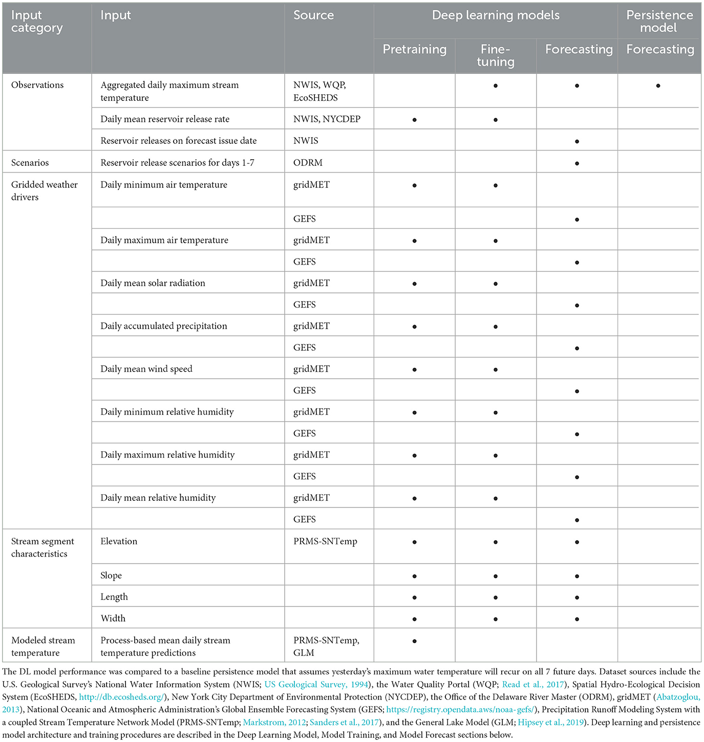
Table 1. Summary of the different datasets used to train the deep learning (DL) models and forecast stream temperature 7 days into the future.
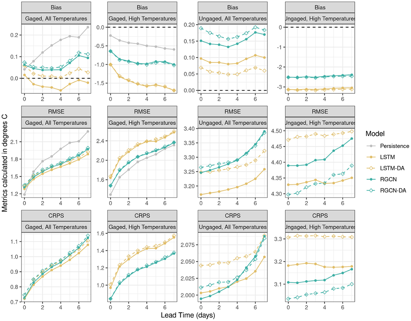
Figure 2. Model forecast accuracy as a function of forecast lead time for gaged and ungaged sites in the Delaware River Basin time for the validation period from 2019-01-03 to 2019-12-23 for persistence model, long short-term memory neural network (LSTM) and recurrent graph convolutional neural network (RGCN) both with and without data assimilation (DA). Accuracy metrics include bias, root mean squared error (RMSE), and continuous ranked probability score (CRPS), each of which is a mean across 5 spatial cross-validation folds and 5 initial seeds for a given model and lead time. High temperatures are observations equal to or above 18°C. Gaged segments were any segments that had observations during training, while ungaged were those that did not have any observations during training.
Deep learning models
We used two different DL model architectures to forecast daily maximum water temperature: a LSTM (Hochreiter and Schmidhuber, 1997) neural network and a spatially-aware variant of the LSTM, the RGCN (Jia et al., 2021). We only briefly describe the LSTM structure because it is described extensively elsewhere (Hochreiter and Schmidhuber, 1997; Rahmani et al., 2020) and in Zwart et al. (2022). The following are the LSTM equations:
where the cell states (ct), and the hidden states (ht) of the LSTM evolve through time and are modified at each time t by a filtered, transformed version of the model inputs at that time, xt (e.g., meteorological drivers and static reach attributes). The LSTM is also given information from previous model timesteps via the previous timestep's hidden and cell states, ht−1 and ct−1. and are learnable weight matrices of the hidden state and input features, respectively, and bg is a learnable bias vector, where g∈{c, f, i, o}. Using the weights and biases, the LSTM generates a forget gate, ft, an input gate, it, and an output gate, ot. represents a temporary memory at time t before filtering the historical information, and ct represents the memory after filtering and combining the historical information using the gate variables ft and it. The information encoded by ct can be used for predictions.
The RGCN alters the calculation of the ct such that the forget gate ft filters historical information not just from its own stream segment, , but also from neighboring segments, , weighted by their level of adjacency; here, this level of adjacency, Aji, is computed from the downstream distance along the network of every segment j relative to segment i . Thus, for the RGCN, equation 8 replaces equation 5:
Generally, the model produces output predictions, ŷ, by using additional hidden layers, such as:
However, we used a unimodal mixture density network (MDN; Bishop, 1994) approach to quantify model prediction uncertainty, following the implementation of MDN for streamflow prediction as described in Klotz et al. (2022). Instead of predicting the maximum daily stream temperature directly, ŷ, we predicted the mean and standard deviation parameters of a Gaussian distribution (μt, σt), which describes the probability of all possible daily maximum stream temperatures at a given timestep. Thus, we use the final layers:
During training, all model weights are incentivized to produce Gaussian parameters that assign high likelihood, , to model targets. In ideal circumstances, this would result in μ parameters that are equal to the observed daily maximum temperature, y (i.e., μ = y ), and very small standard deviations (e.g., σ≈0); if the exact value of the target is hard to predict, then increased standard deviation will likely be the route to maximize likelihood. Although this intuition remains valid (i.e., maximizing the likelihood), in practice the negative log likelihood is minimized for numerical stability:
where N(y|μ(x), σ(x)) is the conditional probability of the observed daily maximum temperature, y, given the Gaussian distribution with parameters μ and σ as a function of the inputs, x. During forecasting, the predicted μ and σ parameters are used to generate samples from the distribution that is compatible with ensemble data assimilation methods (i.e., ensemble Kalman filter).
In conjunction with our MDN probabilistic predictions, we also used Monte Carlo Dropout (MCD). We implemented MCD as described in Gal and Ghahramani (2016), where the DL model randomly removes a proportion of the network's recurrent and input elements (by setting their weights to 0) during each training iteration or prediction activity. When making many predictions using MCD, this produces an ensemble of DL structures and improved forecast uncertainty characterization based on inspecting reliability plots and percent of observations within 90% confidence intervals (CIs) (described in the Model evaluation section).
Data assimilation
During the forecasting period, we used the ensemble Kalman filter (EnKF) as our data assimilation algorithm to update maximum water temperature predictions, hidden, and cell states of the DL as described in Zwart et al. (2022). At each time step, we sample from the predicted probability distribution of daily maximum water temperature to generate ~1,000 ensemble member predictions (validation period = 5 weather ensemble members * 200 samples; testing period = 31 ensemble weather members * 33 samples). These ensemble predictions were compared to observations of daily maximum water temperature, and the temperature predictions and DL model cell states were adjusted using the Kalman gain weighting matrix. After maximum water temperature and model states were updated with the EnKF, the updated states were used to initialize the model states of the DL at the next time step to make new predictions. Both the LSTM and RGCN had a model variation that used this DA method, hereafter called the “LSTM-DA” and “RGCN-DA.” See Zwart et al. (2022) for more detailed description of the EnKF method used in this study.
Model training
We trained the DL models on 70 stream segments of the Delaware River Basin, including management-relevant, gaged, and ungaged segments (Figure 1). Our model was first pre-trained for 50 epochs with modeled stream temperature from 1982-04-01 to 2021-04-14 (excluding 2019 validation year) using the pretraining dataset as the target features and the gridMET historical drivers as the input features. Next, pretrained model weights and biases were fine-tuned using observations of maximum daily water temperature for 350 epochs, using the same gridMET historical drivers from 1982-04-01 to 2021-04-14 (excluding 2019 validation year). Due to permissible size, models were updated with the entire training set, not batches. We used the LSTM and RGCN model structures described above, hidden layer dimensions of 16 for both the recurrent layer and intermediate feedforward layer, recurrent and elemental dropout rates of 0.40, and an Adam learning rate of 0.05 for both phases of training. We trained each model across the 5 spatial cross-validation folds using 5 different starting seeds, resulting in 25 trained models for each model type (e.g., LSTM-DA) in the validation period.
The model hyperparameters (e.g., number of epochs, learning rates, hidden units, and dropout rates) were tuned manually to achieve reasonable model performance and did not differ much from previous welltrained DL models used in the Delaware River Basin (Zwart et al., 2022). We found these hyperparameters and input features to perform well for our DL forecasting models based on examining accuracy and uncertainty quantification metrics (e.g., root mean squared error, model reliability). After the models were trained, the ending DL model states from the fine-tune training phase were used to initialize the DL model states during the start of the forecasting phase. We used PyTorch 1.12.1 to train and forecast with the DL models (Paszke et al., 2019).
Model forecasts
Forecasts were issued retrospectively, but we attempted to mimic operational conditions as closely as possible (e.g., observations of maximum temperature only available from yesterday). On each issue date, we made predictions for the issue date (day 0) and 1 through 7 days into the future using the previous issue date's (day −1) DL model states as the starting conditions (i.e., maximum water temperature, hidden, and cell states). We made predictions using trained LSTM and RGCN models with and without data assimilation (LSTM-DA, RGCN-DA, LSTM, RGCN) as well as a deterministic persistence forecast as our baseline model (Table 1). The persistence model simply forecasts the same maximum water temperature that was observed yesterday for all 8 days that follow. If no observations were observed yesterday, then there was no forecast from the persistence model. If there were observations available on the preceding date (day −1), the LSTM-DA and RGCN-DA models assimilated the observations into the LSTM or RGCN model as described in the data assimilation section and in Zwart et al. (2022).
The DL models had a total of ~1,000 ensemble member predictions, which were generated by sampling 200 (validation period) or 33 (test period) times from the predicted distribution when using each of the 5 or 31 GEFS ensemble members as input features, respectively. Additionally, each of the batches used for the 5 or 31 GEFS ensemble members started at a slightly different hidden and cell state representing uncertainty in model initial conditions. Collectively, the ~1,000-ensemble prediction distribution represents our total forecast uncertainty when considering driver uncertainty, DL model parameter uncertainty, and initial condition uncertainty.
All model training and forecast generation was conducted on USGS Advance Research Computing resources using a combination of central processing units (CPUs) and graphics processing units (GPUs) (Falgout et al., 2019). Model training and forecasting took about 12 hours for all cross-validation and testing models.
Model evaluation
We evaluated model forecast performance as described in Zwart et al. (2022) using bias, RMSE, and continuous ranked probability score [CRPS; Thomas et al. (2020)] calculated from predictions and observations of maximum water temperature. CRPS measures both the accuracy and precision of the full distribution of ensemble predictions (interpreted as a probabilistic forecast), where lower values indicate a better model performance. Each of these metrics was computed for each of the reaches with observations in a validation or test dataset and then averaged across reaches. We averaged metrics for each model across the 5 spatial cross-validation folds and 5 different starting seeds in the validation period; thus, the validation results are a mean of 25 model runs for each model type. Using the results from the validation period, we chose a single model and starting seed with which to run in the test period after re-training the model on all available training data; thus, the testing results are a mean of only one model run.
We evaluated how well the model characterized forecast uncertainty using reliability plots where we calculated the proportion of observations that fell within confidence intervals calculated from the ensemble predictions. A wellcalibrated forecasting model would have 10% of observations within the 10% forecast confidence interval (i.e., the 45–55th quantiles of the forecast probability distribution), 20% of observations in the 20% forecast confidence interval (the 40–60th quantiles), and so on. If a higher or lower percentage of the observations fall within a given forecast confidence interval, then the model is considered underconfident or overconfident, respectively.
Thermal exceedances of 23.89°C (75°F) are of decision-making relevance in the upper Delaware River Basin, so we evaluated our models' performance from a classification perspective using confusion matrices. We determined when the 0.95 quantile (i.e., the upper bound of the 90% CI) did and did not exceed this thermal threshold and compared that to observed (non-)exceedances. Confusion matrices were then calculated, capturing true positives, false positives, true negatives, and false negatives. Here, a true positive was defined as when the 0.95 quantile and observed water temperature were both above the thermal threshold, whereas a false negative was when the 0.95 quantile was below the thermal threshold, but the observed temperature exceeded this threshold. Ideally true positives and negatives are maximized (i.e., 1 proportion of observed) while false positives and negatives are minimized (i.e., 0 proportion of observed). These confusion matrices were considered for 1-day ahead forecasts as these are the most crucial decision-relevant time horizon for reservoir releases.
Model code used to create pretraining process-based datasets, train the DL models, and forecast with the trained DL models can be found at Oliver et al. (2023). All model drivers, observations, and predictions are publicly available Oliver et al. (2022, 2023).
Results
Model validation
Our DL models predicted maximum daily stream temperature for 70 segments with a mean RMSE across all spatial cross-validation folds of 2.03–2.11°C depending on model type for 1-day lead times in the validation period (Figure 2). All DL models performed substantially better at gaged locations compared to ungaged locations as mean RMSE ranged from 1.45 to 1.52°C for gaged sites and 3.18 to 3.27°C for ungaged sites at 1-day lead times (Figure 2). Model accuracy worsened with longer lead times: RMSE ranged from 1.89 to 1.99°C for gaged sites and from 3.26 to 3.39°C for ungaged sites 7 days in the future. Our DL models performed better than the baseline persistence model across all temperatures for 1–7 day lead times, but the persistence model had better performance metrics for RMSE and bias when only considering high temperatures (>18°C).
Of the DL models, the LSTM model was generally the best performing model when considering all temperature observations, as the LSTM model had the lowest RMSE, second lowest bias, and second lowest CRPS for gaged and ungaged locations at 1- and 7-day lead times (Figure 2). For the higher temperature observation subset (>18°C), the RGCN and RGCN-DA models were best performing at gaged locations with nearly identical performance for RMSE, bias, and CRPS at 1- and 7-day lead times. The RGCN-DA was superior for ungaged locations across all metrics and lead times except for RMSE at 5–7 day lead times where the LSTM model was the best performing model (Figure 2). Model performance at freezing or near freezing water temperatures (−1 to 1°C) also showed superior performance for the RGCN model structure as the RGCN had the lowest RMSE averaged across all lead times (gaged = 1.42°C, ungaged = 1.57°C) followed by RGCN-DA (gaged = 1.45°C, ungaged = 1.65°C), LSTM (gaged = 1.64°C, ungaged = 2.41°C), and LSTM-DA (gaged = 1.72°C, ungaged = 2.43°C).
All DL models characterized forecast uncertainty well for gaged locations across all temperature observations and for when only considering high temperature observation subset, with near perfect uncertainty characterization for 1-day lead times (Figure 3); however, all models characterized uncertainty much more poorly at ungaged locations. All model types became more overconfident at longer lead times for gaged locations while ungaged location uncertainty characterization remained roughly the same across all lead times. For gaged locations, the RGCN model characterized uncertainty best when considering all temperature observations while the RGCN-DA model was best for the higher temperature observation subset. For ungaged locations, all models were overconfident, but the RGCN and RGCN-DA were less overconfident compared to the LSTM and LSTM-DA, especially at the higher forecast confidence intervals (Figure 3).
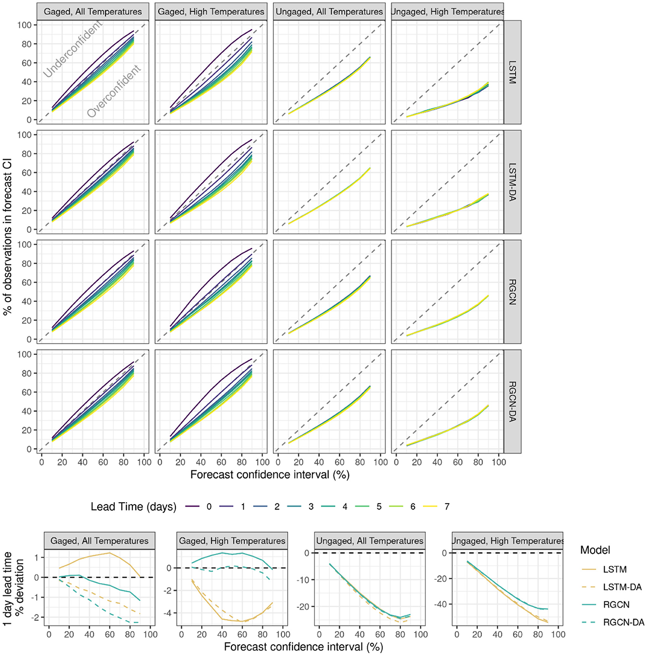
Figure 3. The top 16 panels are reliability plots showing the percentage of observations occurring in each of nine forecast confidence intervals (10% to 90%), for all uncertainty-estimating model types for gaged and ungaged locations and all-temperature and high-temperature observation subsets (>18°C) for the validation period from 2019-01-03 to 2019-12-23. Model types include long short-term memory neural network (LSTM) and recurrent graph convolutional neural network (RGCN) both with and without data assimilation (DA). A model that perfectly characterizes forecast uncertainty would fall along the diagonal dashed 1:1 line. The deviations from the diagonal dashed 1:1 line for the 1-day lead time forecasts across all model types are shown in the bottom panels.
Compared to other DL models, the RGCN-DA was best at forecasting maximum temperature at ungaged locations that were along the mainstem river reaches, especially for higher temperature observation subset (Figure 4). These mainstem river reaches show among-stream variation in annual stream temperature dynamics mostly driven by proximity to upstream reservoirs, and the RGCN-DA model was best at capturing these dynamics, especially during summertime periods (Figure 4). Additionally, the RGCN-DA and RGCN models both performed best at predicting management-relevant thermal exceedance events (>23.89°C) for gaged and ungaged reaches, as the upper bound of the RGCN-DA's 90% confidence interval captured thermal exceedance events 94% of the time for gaged sites and 23% of the time for ungaged sites (Figure 5). This was substantially better performance for the RGCN-DA at ungaged locations compared to the other DL models.
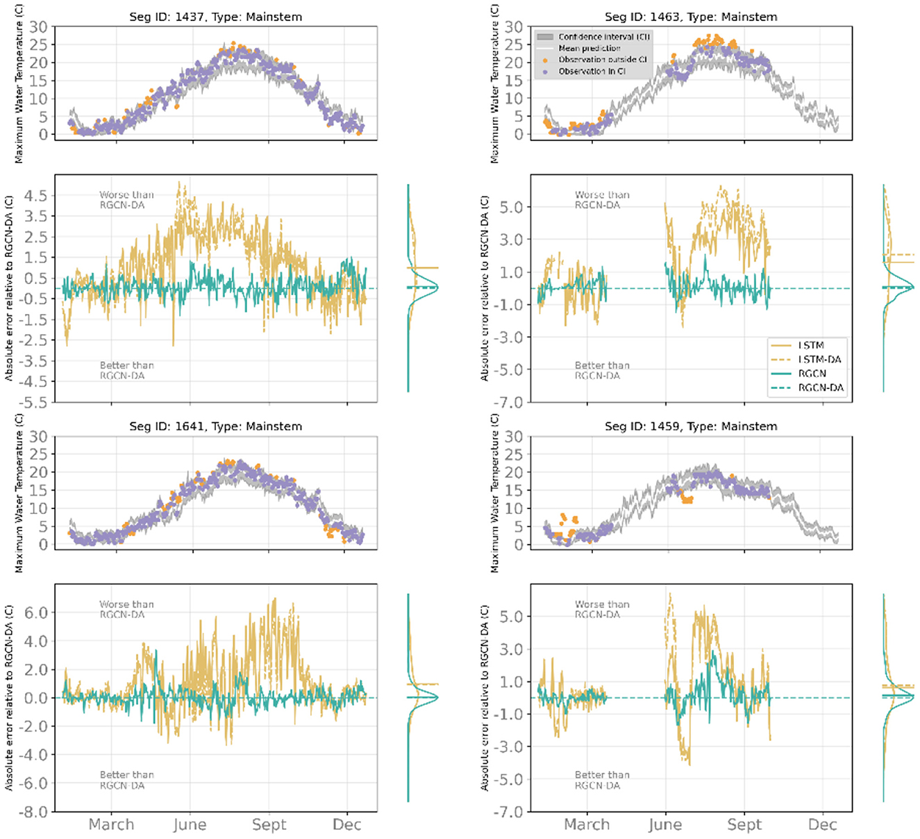
Figure 4. Ungaged, validation set examples of sites along the mainstem highlighting the performance of the recurrent graph convolutional neural network with data assimilation (RGCN-DA) model across four streams. For each stream segment, the top panels consist of maximum water temperature observations and RGCN-DA predictions at 1-day lead time for the validation period from 2019-01-03 to 2019-12-23 where the gray band is a 90% confidence interval (CI), the white line is the mean of all ensemble and sample predictions, observations within the 90% CI are purple, and observations outside the 90% CI are orange. The bottom panels show the deviation of other DL models relative to the RGCN-DA during the validation period and the marginal plots on these panels show distribution and mean of these relative absolute errors. Positive values indicate higher absolute error than the RGCN-DA, whereas negative values indicate lower absolute error than the RGCN-DA.
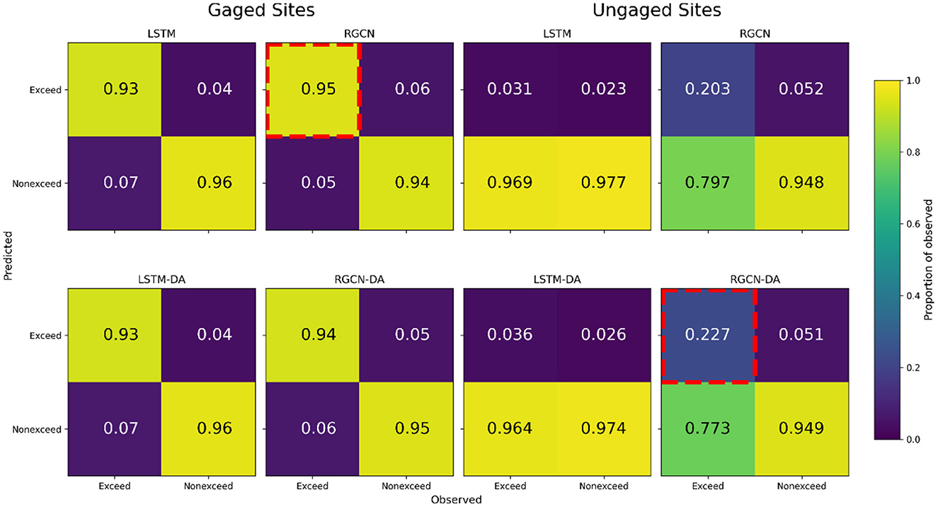
Figure 5. Model comparison of confusion matrices, displaying the ability of 90% confidence intervals to accurately capture thermal exceedances in the Delaware River Basin for long short-term memory neural network (LSTM) and recurrent graph convolutional neural network (RGCN) both with and without data assimilation (DA). Within each confusion matrix, columns are scaled by the number of observed (non-)exceedances. Perfect performance would display 1 in the top left and lower right quadrants with the remaining quadrants equal to 0. For gaged and ungaged sites, the highest proportion of true positives is highlighted by a red, dashed outline.
Considering all validation results, we concluded that the RGCN-DA model was the best performing model for our study location given its superior performance at ungaged locations and higher temperature observation subset along with comparable results at gaged locations and all other temperature observations. The main water temperature concern in the Delaware River Basin is anticipating when water temperatures will exceed thermal tolerances of aquatic organisms, thus we consider the validation results related to high temperature prediction accuracy more strongly. For model testing, we only tested the RGCN-DA model with the test dataset that included 6 ungaged test sites and all other gaged sites from the period of 2021-04-18 to 2022-09-22 and we detail the test results below.
Model test
The RGCN-DA performed well during the test period and in some cases, showed improved results compared to the validation period (Figure 6). For example, RMSE and CRPS at ungaged locations for all temperature and high temperature observation subsets improved compared to the validation period. Additionally, the RGCN-DA had better RMSE compared to the persistence model for 1–7 day lead times during the test period for all temperature and high temperature observation subsets, which was not the case during the validation period. However, RGCN-DA model bias was of higher magnitude for gaged sites and high temperatures compared to the validation period for both the RGCN-DA and the persistence forecast, which generally indicates more difficult forecasting conditions. Although RGCN-DA RMSE was better compared to the persistence model RMSE in the test period, RMSE for both RGCN-DA and persistence model were worse relative to the validation period for all temperature observations and high temperature observation subsets, again indicating more difficult forecasting conditions.
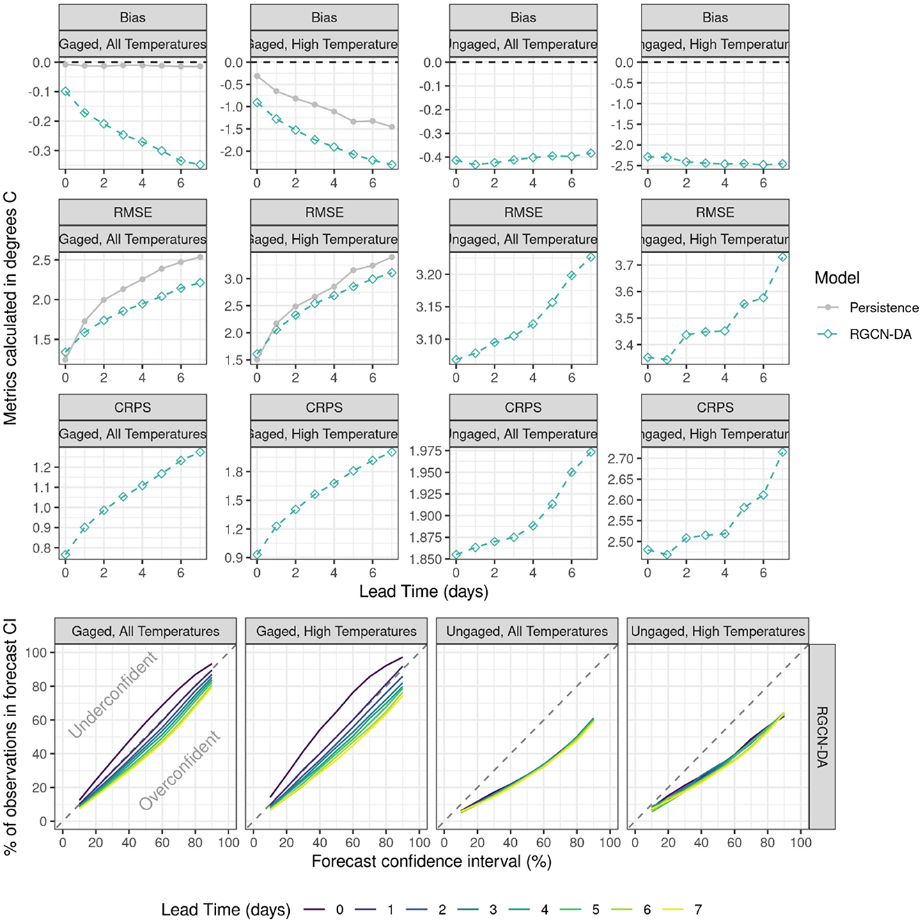
Figure 6. Model forecast accuracy and reliability in the Delaware River Basin during the test period from 2021-04-18 to 2022-09-22 for the recurrent graph convolutional neural network with data assimilation (RGCN-DA) and persistence model. The top twelve panels show model forecast test accuracy as a function of forecast lead time for gaged and ungaged sites and the bottom four panels show model reliability. Accuracy metrics include bias, root mean squared error (RMSE), and continuous ranked probability score (CRPS), and the reliability panels show the percentage of observations occurring in each of nine forecast confidence intervals. A model that perfectly characterizes forecast uncertainty model would fall along the diagonal dashed 1:1 line. High temperatures are observations equal to or above 18°C. Gaged segments were any segment that had observations during training whereas ungaged were those that did not have any observations during training.
The RGCN-DA characterization of forecast uncertainty at gaged sites was consistent between the validation and testing periods with 0-day lead times being slightly underconfident, 1-day lead times being well calibrated, and longer forecast horizons being more overconfident (Figure 6). For ungaged locations, the RGCN-DA model was consistently overconfident with 90% CIs containing the observation ~60% of the time for all temperature observations and 64% of the time for high temperature observation subset. This is an improvement compared to the validation period for high temperature observation subset as the RGCN-DA's 90% CIs contained observations only 46% of the time.
We examined prediction time series for representative headwater, mainstem, and near reservoir gaged and ungaged locations during the test period, which are shown in Figures 7, 8. For gaged locations, the RGCN-DA was generally accurate for mainstem and headwater river reaches, while RGCN-DA forecasts were worse for locations directly downstream from reservoirs (Figure 7). Across all representative gaged locations, the 90% CIs were very reliable with occasional strings of failures that tended to occur in late fall or winter. For ungaged locations, the RGCN-DA forecasts were generally worse across all representative reaches, and observations falling outside the 90% CI were both more common and clustered (Figure 8). The RGCN-DA model performed best for the ungaged mainstem reaches but tended to underpredict summertime temperatures for the headwater reaches and tended to overpredict for the reservoir reaches.
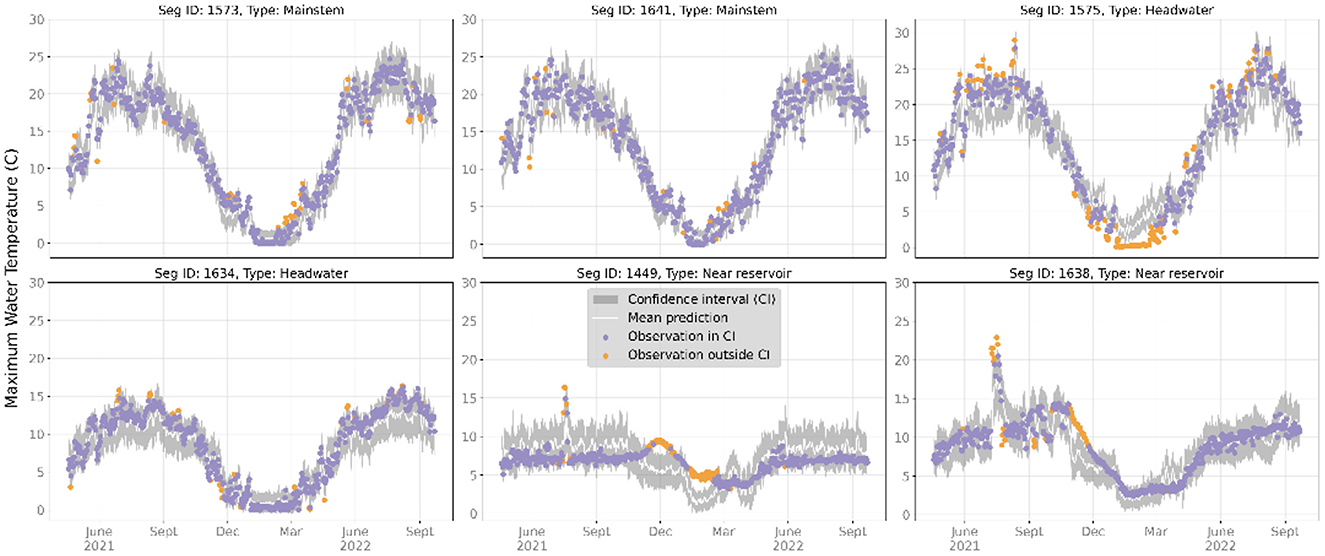
Figure 7. Maximum water temperature observations and recurrent graph convolutional neural network with data assimilation (RGCN-DA) predictions for gaged segments at 1-day lead time for select sites during the test period from 2021-04-18 to 2022-09-22. The gray bands are 90% confidence intervals (CIs) and the white line is the mean of all ensemble and sample predictions. Observations that fall within the 90% CIs are purple, and observations that fall outside of the 90% CI are orange. Stream segments 1,575 and 1,641 were deemed mainstem gages, 1,575 and 1,634 were deemed headwater gages, and 1,449 and 1,638 were deemed reservoir-impacted gages.
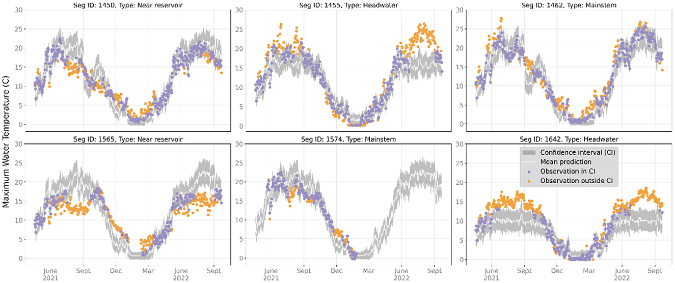
Figure 8. Maximum water temperature observations and recurrent graph convolutional neural network with data assimilation (RGCN-DA) predictions for all ungaged segments at 1-day lead time during the test period from 2021-04-18 to 2022-09-22. The gray bands are 90% CIs (confidence intervals) and the white line is the mean of all ensemble and sample predictions. Observations that fall within the 90% CIs are purple, and observations that fall outside of the 90% CI are orange. Stream segments 1,462 and 1,574 were deemed mainstem gages, 1,455 and 1,642 were deemed headwater gages, and 1,450 and 1,565 were deemed reservoir-impacted gages.
Discussion
Recent work has shown DL models to perform better than other modeling methods when faced with the challenge of predicting aquatic variables in ungaged locations (Kratzert et al., 2019; Rahmani et al., 2021; Feng et al., 2022; Weierbach et al., 2022; Zhang et al., 2022). Given the better performance of DL models, focus on improving DL methods would be beneficial for this prediction challenge. In this paper, we evaluated the performance of four DL models for forecasting daily maximum stream temperature at both gaged and ungaged locations, which included two DL model architectures both with and without data assimilation (i.e., ensemble Kalman filter). To the best of our knowledge, this is the first evaluation of DL models at ungaged locations for stream network water temperature forecasts. Below we discuss the forecast performance of these DL models for this prediction challenge and future research opportunities.
All DL models performed well when forecasting maximum daily stream temperature for 70 segments in the Delaware River Basin with a mean RMSE of 1.49°C and CRPS of 0.83°C for day-ahead forecasts across gaged locations and performed modestly well for ungaged locations with a mean RMSE of 3.24°C and CRPS of 2.02°C for day-ahead forecasts. The gaged location accuracy is similar in performance to previous temperature forecasting approaches (e.g., Cole et al., 2014; Zwart et al., 2022), and we are unaware of other studies that have evaluated forecasts of daily maximum stream temperature for ungaged locations. Although all 70 sites were within 1 degree latitude and longitude of each other, daily maximum stream temperature varied a lot due to reservoir effects and natural variability (e.g., groundwater inflow). For example, the month with the warmest mean stream temperature (July) ranged from 25.2°C at the warmest stream segment to 7.4°C at the coolest segment. Despite this >17°C difference among stream segments in water temperature during the warmest months, our DL models were able to capture inter-segment variability in this highly thermally altered stream network.
DL model architecture had the largest effect on forecast performance for the highest and lowest temperature observation subsets as the RGCN-DA and RGCN consistently outperformed other models when making forecasts for temperatures greater than 18°C. The RGCN-DA had the lowest CRPS and RMSE for forecasting temperatures above 18°C at ungaged locations. Model performance at higher temperatures is important in the Delaware River Basin because water resource managers make decisions about when and how much water to release from reservoirs to cool downstream segments. Additionally, accurate network-wide forecasts of stream temperature at higher temperature regimes could inform the public on when and where catch and release fishing may be most suitable to avoid thermal stress on fishes. Of note, the value of DA was only examined with regards to the EnKF method, and alternative approaches that are more integrated with model training process may be superior to this more general method (e.g., Nearing et al., 2021a).
The RGCN architecture, with and without DA, performed best around freezing temperatures (−1 to 1°C) and may have an advantage over the LSTM at these temperature regimes because external drivers are typically decoupled from water temperature dynamics near freezing temperatures (Letcher et al., 2016); thus, added network structure may help maintain accurate predictions despite this decoupling. Accurate predictions of water temperature near freezing can be important for predicting the location, magnitude, and timing of river ice cover and thaw. Similar to high temperature regimes, these freezing temperatures can affect recreation, tourism, and wildlife. Under some conditions ice in a river network can jam, forming a dam and impounding water, which introduces a risk of flooding (Beltaos, 1995). For hydropower dams, river ice can block or damage pipes and turbines and pose additional operational constraints and reductions in power production (Gebre et al., 2013). Although streams in the Delaware River Basin are not highly prone to freezing, the improved RGCN forecasts at near freezing temperatures may be useful if model performance is similar in other basins.
Model results indicated that the RGCN and DA may leverage nearby information to improve predictions for ungaged locations. Of the 16 segments that were used in the spatial cross-validation, the RGCN was the best performing DL model structure for 11 of the segments when they were ungaged, and 5 of these 11 segments had the LSTM as the best performing model when the segments were gaged (Figure 9). This contrasts with only five segments that had an LSTM model as the best performing model when the segments were ungaged. Additionally, DA improved predictions for two of the segments that had the LSTM as the best performing model when ungaged. Topp et al. (2023) show that non-local information accounts for greater than two-thirds of prediction influence for RGCN models in the Delaware River Basin. Indeed, this non-local information may help improve forecasts of stream temperature at ungaged sites by leveraging information from nearby sites. Despite improved predictions for the RGCN compared to LSTM at many ungaged locations, overall forecast performance at ungaged locations was much lower than gaged locations. DL forecasts at ungaged locations might be improved with larger training datasets over the 70 segments we used in this study, segment characteristics that distinguish unique aspects of segments in this basin (e.g., groundwater influence), or potentially different network architecture models that may better reflect real-world river network (e.g., Graph WaveNet; Wu et al., 2019; Topp et al., 2023). Improvements to input data might also interact with differences among model architectures; for example, a wider range of segment characteristics could improve LSTM performance and thus narrow the accuracy difference between LSTM and RGCN or Graph WaveNet models. Also, past work has shown that pretraining is more powerful for conditions and locations for which data are sparse (Read et al., 2019; Jia et al., 2021) and that a mediocre source of pretraining data (e.g., a process-based model that omits key features such as reservoirs) could introduce errors that are not unlearned by few true observations. However, we are unaware of a robust analysis on the value of different pretraining datasets on DL model performance under various data sparsity conditions. In the context of machine learning literature, this 70-site study area is relatively small; and although the Delaware River Basin is wellmonitored, many of its sites have sparse or inconsistent water temperature records. Both model architectures likely would benefit from increased data availability, and we hypothesize that the RGCN-DA would exhibit the greatest improvements due to its additional spatial data integration. Conversely, we expect that reduced data availability and diversity would decrease ungaged prediction performance.
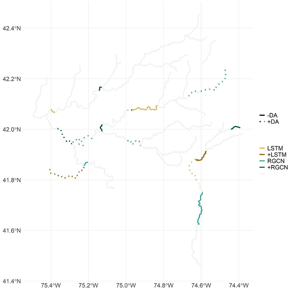
Figure 9. Map showing all the stream segments used as ungaged locations in one of the spatial cross-validation folds. Segments are colored based on what deep learning (DL) model structure was most accurate when the segment was ungaged. Darker colors indicate that the segment's most accurate DL model structure changed when switching from gaged to ungaged where +LSTM indicates that the long short-term memory neural network (LSTM) was more accurate when the segment was ungaged, whereas the recurrent graph convolutional neural network (RGCN) was more accurate when gaged. Segment line style indicates whether data assimilation (DA) accompanied the DL model structure as the most accurate model for ungaged predictions where +DA means that DA was more accurate when the segment was ungaged, whereas no DA was more accurate when the segment was gaged. The gray segments indicate all other forecast segments used in this study.
Our DL models characterized uncertainty well at gaged locations with 88–90% of observations included in the 90% CIs at 1-day lead time. However, our DL models were overconfident at ungaged locations as 65–67% of observations were contained in the 90% CIs. Although ungaged performance was worse, this was not specific to uncertainty or CIs, and this likely indicates that additional work would be helpful to characterize ungaged streams with better input features. The unimodal Gaussian approach for characterizing target uncertainty is a convenient extension of mean squared error optimization, which allows the model to explicitly learn and provide a bound of uncertainty with little additional burden. Our gaged uncertainty results are good, adding support to the MDN approach inspired from Klotz et al. (2022); however, initial explorations indicated very equal performance between Gaussian and Laplacian approaches for our stream temperature task (which is less tail-heavy than rainfall and runoff), and we saw additional benefit when combining MCD with Gaussian uncertainty.
Although our models characterized uncertainty well, gaged uncertainty quantification tended to be worst at either the highest forecast CI (90% CI, downward deviation curve, Figure 3) or moderate forecast CI (40–60%, u- or n-shaped deviation curves) for cross-validation results. Using the Gaussian distribution approximation of our MDN predictions, overconfidence at high confidence intervals likely indicates a limitation in the predicted standard deviation, which may not accurately represent some of the less common stream temperature values. Under- or overconfidence at intermediate confidence intervals likely indicates a shortcoming in the predicted mean. For gaged sites, low forecast CIs were relatively reliable; but for ungaged sites, the low forecast CIs were relatively unreliable and displayed worsening reliability at higher forecast CIs. This was likely representative of the broader problem of difficult spatial generalization for both predicted mean and standard deviation parameters.
As forecast lead times increased, the DL models became more overconfident. This can be due to higher error at greater lead times or may represent a loss of uncertainty introduced by taking sample means from earlier days as the current day's autoregressive input. A brief, initial exploration of using all predicted samples (rather than sample means) indicated improved CI reliability, but with prohibitively increased computational and memory burdens, which we want to avoid to show clear computational benefits over full Markov chain Monte Carlo approaches. Another option for improving uncertainty characterization at longer lead times would be to train separate models for making predictions at longer lead times; DL model distribution predictions are expected to adjust variance appropriately to maximize the likelihood loss function at these longer lead times and we might expect our models to become less overconfident. Although not demonstrated here, having distribution parameters as outputs is highly appealing for interrogating what is contributing most to model forecast uncertainty. Explainable artificial intelligence (XAI) methods such as expected gradients (Erion et al., 2021) could be used to assign attribution of increased or decreased uncertainty parameters to inputs (e.g., precipitation contributes most to the predicted variance of stream temperature). This would be analogous other forecast uncertainty partitioning (Heilman et al., 2022), which can help improve forecasts by focusing efforts on the most important contributors to uncertainty (Bauer et al., 2015).
Data availability statement
The datasets presented in this study can be found in online repositories. The names of the repository/repositories and accession number(s) can be found below: https://www.sciencebase.gov/catalog/item/623e4418d34e915b67d7dd78 and https://www.sciencebase.gov/catalog/item/6238fcead34e915b67cc4856.
Author contributions
JZ, JD, SH, SO, AA, and EW contributed to conception and design of the study. JD led the deep learning model development. JZ, JD, SH, SO, JCR, MS, AA, HC-D, XJ, JS, TT, DW, and EW contributed code to data preparation, model evaluation, and/or figure generation. MS and SO led the data releases. JZ wrote the first draft of the manuscript. JD, SH, EW AA, SO, and DW wrote sections of the manuscript. All authors contributed to manuscript revision, read, and approved the submitted version.
Acknowledgments
All model training was run on USGS High Performance Computing. We thank Jared Willard, Fredrick Cheng, and two reviewers for constructive feedback on previous versions of this manuscript. Any use of trade, firm, or product names is for descriptive purposes only and does not imply endorsement by the U.S. Government.
Conflict of interest
The authors declare that the research was conducted in the absence of any commercial or financial relationships that could be construed as a potential conflict of interest.
Publisher's note
All claims expressed in this article are solely those of the authors and do not necessarily represent those of their affiliated organizations, or those of the publisher, the editors and the reviewers. Any product that may be evaluated in this article, or claim that may be made by its manufacturer, is not guaranteed or endorsed by the publisher.
References
Abatzoglou, J. T. (2013). Development of gridded surface meteorological data for ecological applications and modelling. Int. J. Climatol. 33, 121–131. doi: 10.1002/joc.3413
Appling, A. P., Oliver, S. K., Read, J. S., Sadler, J. M., and Zwart, J. A. (2022). “Machine Learning for Understanding Inland Water Quantity, Quality, and Ecology,” in Encyclopedia of Inland Waters, eds. K. S. Cheruvelil, K. Tockner, and T. Mehner (UK: Elsevier), 585–606.
Bauer, P., Thorpe, A., and Brunet, G. (2015). The quiet revolution of numerical weather prediction. Nature 525, 47–55. doi: 10.1038/nature14956
Bishop, C. M. (1994). Mixture density networks. Technical Report, Aston University, Birmingham, United Kingdom. Available online at: https://publications.aston.ac.uk/id/eprint/373/
Boyd, J. W., Guy, C. S., Horton, T. B., and Leathe, S. A. (2010). Effects of catch-and-release angling on salmonids at elevated water temperatures. North Am. J. Fisher. Manage. 30, 898–907. doi: 10.1577/M09-107.1
Breece, M. W., Oliver, M. J., Fox, D. A., Hale, E. A., Haulsee, D. E., Shatley, M., et al. (2021). A satellite-based mobile warning system to reduce interactions with an endangered species. Ecologic. Applicat. 31, 2358. doi: 10.1002/eap.2358
Chen, S., Appling, A., Oliver, S., Corson-Dosch, H., Read, J., Sadler, J., et al. (2021). “Heterogeneous stream-reservoir graph networks with data assimilation,” in 2021 IEEE International Conference on Data Mining (ICDM) (New York, NY: IEEE), 1024–1029.
Cole, J. C., Maloney, K. O., Schmid, M., and McKenna, J. E. (2014). Developing and testing temperature models for regulated systems: a case study on the Upper Delaware River. J. Hydrol. 519, 588–598. doi: 10.1016/j.jhydrol.2014.07.058
Daw, A., Thomas, R. Q., Carey, C. C., Read, J. S., Appling, A. P., and Karpatne, A. (2020). “Physics-guided architecture (pga) of neural networks for quantifying uncertainty in lake temperature modeling,” in Proceedings of the 2020 Siam International Conference on Data Mining (SIAM), 532–540.
Dietze, M. C., Fox, A., Beck-Johnson, L. M., Betancourt, J. L., Hooten, M. B., Jarnevich, C. S., et al. (2018). Iterative near-term ecological forecasting: Needs, opportunities, and challenges. Proc. Natl. Acad. Sci. U.S.A. 115, 1424–1432. doi: 10.1073/pnas.1710231115
Erion, G., Janizek, J. D., Sturmfels, P., Lundberg, S. M., and Lee, S.-I. (2021). Improving performance of deep learning models with axiomatic attribution priors and expected gradients. Nat. Mach. Intell. 3, 620–631. doi: 10.1038/s42256-021-00343-w
Falgout, J. T., Gordon, J., Davis, M. J., Williams, B., and USGS Advanced Research Computing. (2019). USGS Tallgrass Supercomputer. doi: 10.5066/P9XE7ROJ
Fang, K., and Shen, C. (2020). Near-real-time forecast of satellite-based soil moisture using long short-term memory with an adaptive data integration kernel. J. Hydrometeorol. 21, 399–413. doi: 10.1175/JHM-D-19-0169.1
Feng, D., Beck, H., Lawson, K., and Shen, C. (2022). The suitability of differentiable, learnable hydrologic models for ungauged regions and climate change impact assessment. Catch. Hydrol. Modell. Approach. 2, 245. doi: 10.5194/hess-2022-245
Feng, D., Fang, K., and Shen, C. (2020). Enhancing streamflow forecast and extracting insights using long-short term memory networks with data integration at continental scales. Water Resour. Res. 56, 793. doi: 10.1029/2019WR026793
Feng, D., Lawson, K., and Shen, C. (2021). Mitigating prediction error of deep learning streamflow models in large data-sparse regions with ensemble modeling and soft data. Geophysic. Res. Lett. 48, 29. doi: 10.1029/2021GL092999
Gal, Y., and Ghahramani, Z. (2016). “Dropout as a bayesian approximation: Representing model uncertainty in deep learning,” in International Conference on Machine Learning (PMLR), 1050–1059.
Gale, M. K., Hinch, S. G., and Donaldson, M. R. (2013). The role of temperature in the capture and release of fish: temperature effects on capture-release. Fish Fisher. 14, 1–33. doi: 10.1111/j.1467-2979.2011.00441.x
Gebre, S., Alfredsen, K., Lia, L., Stickler, M., and Tesaker, E. (2013). Review of ice effects on hydropower systems. J. Cold Reg. Eng. 27, 196–222. doi: 10.1061/(ASCE)CR.1943-5495.0000059
Guo, G., Liu, S., Wu, Y., Li, J., Zhou, R., and Zhu, X. (2018). Short-term water demand forecast based on deep learning method. J. Water Resour. Plann. Manage. 144, 04018076. doi: 10.1061/(ASCE)WR.1943-5452.0000992
Heilman, K. A., Dietze, M. C., Arizpe, A. A., Aragon, J., Gray, A., Shaw, J. D., et al. (2022). Ecological forecasting of tree growth: Regional fusion of tree-ring and forest inventory data to quantify drivers and characterize uncertainty. Global Change Biol. 28, 2442–2460. doi: 10.1111/gcb.16038
Hipsey, M. R., Bruce, L. C., Boon, C., Busch, B., Carey, C. C., Hamilton, D. P., et al. (2019). A general lake model (GLM 3.0) for linking with high-frequency sensor data from the global lake ecological observatory network (GLEON). Geosci. Model Dev. 12, 473–523. doi: 10.5194/gmd-12-473-2019
Hochreiter, S., and Schmidhuber, J. (1997). Long short-term memory. Neural Computat. 9, 1735–1780. doi: 10.1162/neco.1997.9.8.1735
Hrachowitz, M., Savenije, H. H. G., Blöschl, G., McDonnell, J. J., Sivapalan, M., Pomeroy, J. W., et al. (2013). A decade of Predictions in ungauged basins (PUB)—a review. Hydrologic. Sci. J. 58, 1198–1255. doi: 10.1080/02626667.2013.803183
Jager, H. I., and Smith, B. T. (2008). Sustainable reservoir operation: can we generate hydropower and preserve ecosystem values? River Res. Applic. 24, 340–352. doi: 10.1002/rra.1069
Jeanson, A. L., Lynch, A. J., Thiem, J. D., Potts, W. M., Haapasalo, T., Danylchuk, A. J., et al. (2021). A bright spot analysis of inland recreational fisheries in the face of climate change: learning about adaptation from small successes. Rev. Fish. Biol. Fisheries 31, 181–200. doi: 10.1007/s11160-021-09638-y
Jia, X., Zwart, J., Sadler, J., Appling, A., Oliver, S., Markstrom, S., et al. (2021). “Physics-guided recurrent graph model for predicting flow and temperature in river networks,” in Proceedings of the 2021 SIAM International Conference on Data Mining (SDM) (SIAM), 612–620.
Karniadakis, G. E., Kevrekidis, I. G., Lu, L., Perdikaris, P., Wang, S., and Yang, L. (2021). Physics-informed machine learning. Nat. Rev. Phys. 3, 422–440. doi: 10.1038/s42254-021-00314-5
Kim, T., Shin, J., Lee, D., Kim, Y., Na, E., Park, J., et al. (2022). Simultaneous feature engineering and interpretation: forecasting harmful algal blooms using a deep learning approach. Water Res. 215, 118289. doi: 10.1016/j.watres.2022.118289
Klotz, D., Kratzert, F., Gauch, M., Keefe Sampson, A., Brandstetter, J., Klambauer, G., et al. (2022). “Uncertainty estimation with deep learning for rainfall–runoff modelling,” in Catchment HYDROLOGY/MODELLING APPROACHES.
Kratzert, F., Klotz, D., Herrnegger, M., Sampson, A. K., Hochreiter, S., and Nearing, G. S. (2019). Toward improved predictions in ungauged basins: exploiting the power of machine learning. Water. Resour. Res. 55, 11344–11354. doi: 10.1029/2019WR026065
Lawrence, G. B., Burns, D. A., Baldigo, B. P., Murdoch, P. S., and Lovett, G. M. (2001). Controls of stream chemistry and fish populations in the Neversink watershed, Catskill Mountains, New York. U.S. Geological Survey.
Letcher, B. H., Hocking, D. J., O'Neil, K., Whiteley, A. R., Nislow, K. H., and O'Donnell, M. J. (2016). A hierarchical model of daily stream temperature using air-water temperature synchronization, autocorrelation, and time lags. PeerJ. 4, e1727. doi: 10.7717/peerj.1727
Markstrom, S. L. (2012). P2S–coupled Simulation with the Precipitation-Runoff Modeling System (PRMS) and the Stream Temperature Network (SNTemp) Models. US Department of the Interior, US Geological Survey.
Meyer, H., and Pebesma, E. (2021). Predicting into unknown space? estimating the area of applicability of spatial prediction models. Methods Ecol. Evol. 12, 1620–1633. doi: 10.1111/2041-210X.13650
Nearing, G. S., Klotz, D., Sampson, A. K., Kratzert, F., Gauch, M., Frame, J. M., et al. (2021a). Technical Note: Data assimilation and autoregression for using near-real-time streamflow observations in long short-term memory networks. Hydrol. Earth Syst. Sci. Discuss. 21, 1–25. doi: 10.5194/hess-2021-515
Nearing, G. S., Kratzert, F., Sampson, A. K., Pelissier, C. S., Klotz, D., Frame, J. M., et al. (2021b). What role does hydrological science play in the age of machine learning? Water Resourc. Res. 57, e2020WR028091. doi: 10.1029/2020WR028091
Nevo, S., Morin, E., Gerzi Rosenthal, A., Metzger, A., Barshai, C., Weitzner, D., et al. (2022). Flood forecasting with machine learning models in an operational framework. Hydrol. Earth Syst. Sci. 26, 4013–4032. doi: 10.5194/hess-26-4013-2022
Olden, J. D., and Naiman, R. J. (2010). Incorporating thermal regimes into environmental flows assessments: modifying dam operations to restore freshwater ecosystem integrity: incorporating thermal regimes in environmental flows assessments. Freshwater Biol. 55, 86–107. doi: 10.1111/j.1365-2427.2009.02179.x
Oliver, S. K., Sleckman, M. J., Appling, A. P., Corson-Dosch, H. R., Zwart, J. A., Thompson, T. P., et al. (2022). Data to support water quality modeling efforts in the Delaware River Basin. doi: 10.5066/P9GUHX1U
Oliver, S. K., Zwart, J. A., Appling, A. P., and Sleckman, M. J. (2023). Predictions and Supporting Data for Network-Wide 7-Day Ahead Forecasts of Water Temperature in the Delaware River Basin. U. S. Geological Survey. doi: 10.5066/P9NVEA4V
Paszke, A., Gross, S., Massa, F., Lerer, A., Bradbury, J., Chanan, G., et al. (2019). Pytorch: an imperative style, high-performance deep learning library. Adv. Neural Informat. PROCESS. Syst. 32, 259. Available online at: https://proceedings.neurips.cc/paper_files/paper/2019/file/bdbca288fee7f92f2bfa9f7012727740-Paper.pdf
Rahmani, F., Lawson, K., Ouyang, W., Appling, A., Oliver, S., and Shen, C. (2020). Exploring the exceptional performance of a deep learning stream temperature model and the value of streamflow data. Environ. Res. Lett. 26, 501. doi: 10.1088/1748-9326/abd501
Rahmani, F., Shen, C., Oliver, S., Lawson, K., and Appling, A. (2021). Deep learning approaches for improving prediction of daily stream temperature in data-scarce, unmonitored, and dammed basins. Hydrologic. Processes 35, 144. doi: 10.1002/hyp.14400
Read, E. K., Carr, L., De Cicco, L., Dugan, H. A., Hanson, P. C., Hart, J. A., et al. (2017). Water quality data for national-scale aquatic research: The Water Quality Portal. Water Resour. Res. 53, 1735–1745. doi: 10.1002/2016WR019993
Read, J. S., Jia, X., Willard, J., Appling, A. P., Zwart, J. A., Oliver, S. K., et al. (2019). Process-guided deep learning predictions of lake water temperature. Water Resour. Res. 55, 9173–9190. doi: 10.1029/2019WR024922
Regan, R. S., Markstrom, S. L., Hay, L. E., Viger, R. J., Norton, P. A., Driscoll, J. M., et al. (2018). Description of the national hydrologic model for use with the precipitation-runoff modeling system (prms). US Geologic. Survey. 18, 9. doi: 10.3133/tm6B9
Sanders, M. J., Markstrom, S. L., Regan, R. S., and Atkinson, R. D. (2017). Documentation of a daily mean stream temperature module—an enhancement to the precipitation-runoff modeling system. US Geologic. Survey 17, 4. doi: 10.3133/tm6D4
Sivapalan, M., Takeuchi, K., Franks, S. W., Gupta, V. K., Karambiri, H., Lakshmi, V., et al. (2003). IAHS Decade on Predictions in Ungauged Basins (PUB), 2003–2012: Shaping an exciting future for the hydrological sciences. Hydrologic. Sci. J. 48, 857–880. doi: 10.1623/hysj.48.6.857.51421
St. John White, B., Paola Ferreri, C., Lellis, W. A., Wicklow, B. J., and Cole, J. C. (2017). Geographic variation in host fish use and larval metamorphosis for the endangered dwarf wedgemussel. Aquatic. Conserv. Mar. Freshw. Ecosyst. 27, 909–918. doi: 10.1002/aqc.2782
Sun, A. Y., Jiang, P., Mudunuru, M. K., and Chen, X. (2021). Explore Spatio-temporal learning of large sample hydrology using graph neural networks. Water Resour. Res. 57, 394. doi: 10.1029/2021WR030394
Thomas, R. Q., Figueiredo, R. J., Daneshmand, V., Bookout, B. J., Puckett, L. K., and Carey, C. C. (2020). A near-term iterative forecasting system successfully predicts reservoir hydrodynamics and partitions uncertainty in real time. Water Resour. Res. 56, 138. doi: 10.1029/2019WR026138
Topp, S. N., Barclay, J., Diaz, J., Sun, A. Y., Jia, X., Lu, D., et al. (2023). Stream temperature prediction in a shifting environment: explaining the influence of deep learning architecture. Water Resour. Res. 59, e2022WR033880. doi: 10.1029/2022W. R.033880
Varadharajan, C., Appling, A. P., Arora, B., Christianson, D. S., Hendrix, V. C., Kumar, V., et al. (2022). Can machine learning accelerate process understanding and decision-relevant predictions of river water quality? Hydrologic. Process. 36, 145. doi: 10.1002/hyp.14565
Viger, R. J. (2014). Preliminary spatial parameters for PRMS based on the Geospatial Fabric, NLCD2001, and SSURGO.
Viger, R. J., and Bock, A. (2014). GIS Features of the Geospatial Fabric for National Hydrologic Modeling.
Weierbach, H., Lima, A. R., Willard, J. D., Hendrix, V. C., Christianson, D. S., Lubich, M., et al. (2022). Stream temperature predictions for river basin management in the pacific northwest and mid-atlantic regions using machine learning. Water 14, 1032. doi: 10.3390/w14071032
Willard, J., Jia, X., Xu, S., Steinbach, M., and Kumar, V. (2022). Integrating scientific knowledge with machine learning for engineering and environmental systems. ACM Comput. Surv. 22, 3514228. doi: 10.1145/3514228
Willard, J. D., Read, J. S., Appling, A. P., Oliver, S. K., Jia, X., and Kumar, V. (2021). Predicting water temperature dynamics of unmonitored lakes with meta-transfer learning. Water Resour. Res. 57, 79. doi: 10.1029/2021WR029579
Williamson, T. N., and Lant, J. G. (2015). User manuals for the delaware river basin water availability tool for environmental resources (DRB–WATER) and associated WATER application utilities. US Geologic. Survey. 15, 1196. doi: 10.3133/ofr20151196
Wu, Z., Pan, S., Long, G., Jiang, J., and Zhang, C. (2019). “Graph WaveNet for Deep Spatial-Temporal Graph Modeling,” in Proceedings of the Twenty-Eighth International Joint Conference on Artificial Intelligence (Macao, China: International Joint Conferences on Artificial Intelligence Organization), 1907–1913.
Xiang, Z., and Demir, I. (2020). Distributed long-term hourly streamflow predictions using deep learning – a case study for State of Iowa. Environ. Modell. Softw. 131, 104761. doi: 10.1016/j.envsoft.2020.104761
Zhang, Y., Ragettli, S., Molnar, P., Fink, O., and Peleg, N. (2022). Generalization of an Encoder-Decoder LSTM model for flood prediction in ungauged catchments. J. Hydrol. 614, 128577. doi: 10.1016/j.jhydrol.2022.128577
Zhi, W., Feng, D., Tsai, W.-P., Sterle, G., Harpold, A., Shen, C., et al. (2021). From hydrometeorology to river water quality: can a deep learning model predict dissolved oxygen at the continental scale? Environ. Sci. Technol. 55, 2357–2368. doi: 10.1021/acs.est.0c06783
Keywords: deep learning—artificial neural network, forecast, data assimilation, water temperature, unmonitored catchment
Citation: Zwart JA, Diaz J, Hamshaw S, Oliver S, Ross JC, Sleckman M, Appling AP, Corson-Dosch H, Jia X, Read J, Sadler J, Thompson T, Watkins D and White E (2023) Evaluating deep learning architecture and data assimilation for improving water temperature forecasts at unmonitored locations. Front. Water 5:1184992. doi: 10.3389/frwa.2023.1184992
Received: 13 March 2023; Accepted: 30 May 2023;
Published: 23 June 2023.
Edited by:
Francesco Granata, University of Cassino, ItalyReviewed by:
Senlin Zhu, Yangzhou University, ChinaMohammad Najafzadeh, Graduate University of Advanced Technology, Iran
Georgia A. Papacharalampous, National Technical University of Athens, Greece
Copyright © 2023 Zwart, Diaz, Hamshaw, Oliver, Ross, Sleckman, Appling, Corson-Dosch, Jia, Read, Sadler, Thompson, Watkins and White. This is an open-access article distributed under the terms of the Creative Commons Attribution License (CC BY). The use, distribution or reproduction in other forums is permitted, provided the original author(s) and the copyright owner(s) are credited and that the original publication in this journal is cited, in accordance with accepted academic practice. No use, distribution or reproduction is permitted which does not comply with these terms.
*Correspondence: Jacob A. Zwart, anp3YXJ0QHVzZ3MuZ292