Application of machine learning and deep neural networks for spatial prediction of groundwater nitrate concentration to improve land use management practices

Karimanzira, Divas; Weis, Jonas; Wunsch, Andreas; Ritzau, Linda; Liesch, Tanja; Ohmer, Marc

doi:10.3389/frwa.2023.1193142

ORIGINAL RESEARCH article

Front. Water, 13 July 2023

Sec. Water and Artificial Intelligence

Volume 5 - 2023 | https://doi.org/10.3389/frwa.2023.1193142

Application of machine learning and deep neural networks for spatial prediction of groundwater nitrate concentration to improve land use management practices

$\r\nDivas Karimanzira$ Divas Karimanzira¹^*

Jonas Weis²

¹Fraunhofer Institute of Optronics, System Technologies and Image Exploitation IOSB, Ilmenau, Germany
²Institut für Angewandte Geowissenschaften (AGW) - Abteilung Hydrogeologie, KIT - Karlsruher Institut für Technologie, Karlsruhe, Germany

The prediction of groundwater nitrate concentration's response to geo-environmental and human-influenced factors is essential to better restore groundwater quality and improve land use management practices. In this paper, we regionalize groundwater nitrate concentration using different machine learning methods (Random forest (RF), unimodal 2D and 3D convolutional neural networks (CNN), and multi-stream early and late fusion 2D-CNNs) so that the nitrate situation in unobserved areas can be predicted. CNNs take into account not only the nitrate values of the grid cells of the observation wells but also the values around them. This has the added benefit of allowing them to learn directly about the influence of the surroundings. The predictive performance of the models was tested on a dataset from a pilot region in Germany, and the results show that, in general, all the machine learning models, after a Bayesian optimization hyperparameter search and training, achieve good spatial predictive performance compared to previous studies based on Kriging and numerical models. Based on the mean absolute error (MAE), the random forest model and the 2DCNN late fusion model performed best with an MAE (STD) of 9.55 (0.367) mg/l, R² = 0.43 and 10.32 (0.27) mg/l, R² = 0.27, respectively. The 3DCNN with an MAE (STD) of 11.66 (0.21) mg/l and largest resources consumption is the worst performing model. Feature importance learning from the models was used in conjunction with partial dependency analysis of the most important features to gain greater insight into the major factors explaining the nitrate spatial variability. Large uncertainties in nitrate prediction have been shown in previous studies. Therefore, the models were extended to quantify uncertainty using prediction intervals (PIs) derived from bootstrapping. Knowledge of uncertainty helps the water manager reduce risk and plan more reliably.

1. Introduction

According to the EU Nitrates Directives, based on data from 2012 to 2015, a quarter of the groundwater bodies in the EU have a poor chemical status, with ~13% primarily contaminated by nitrate above 50 mg/l (EC, 2018). From 2016 to 2018, there was only a slight improvement, according to the report of the BMU for 2020 (BMU and BMEL, 2020). Groundwater management is a difficult task because groundwater processes are slow and the impact of anthropogenic activities and contaminants from the surface sometimes appears only in the long term. As a result, the EU Water Framework Directive (WFD) recommends that environmental measures be implemented to prevent groundwater nitrate pollution in the first place and thus contribute to aquifer quality (Directive 2006/118/EC, 2006; Alcalá and Custodio, 2015). This means that risk-prone areas for contamination from anthropogenic sources (e.g., agriculture) should be identified using models, making the modeling and prediction of groundwater nitrate, even in unmeasured areas, a critical management task for environmental planning. Implementing such models can be a significant agri-environmental measure with far-reaching implications for aquifer planning.

Sustainable groundwater management is only possible if environmental agencies, groundwater managers, and land users cooperate and work together in a finger-pointing information system. The groundwater managers should be able to pinpoint influencing factors such as land use as a cause for an increase in nitrate concentration so that the farmers, on the other hand, can reduce excessive fertilization of crops, generating surplus nutrient flow that ends up polluting the groundwater system. This is only possible if the groundwater managers have decision tools to spatially predict the nitrate concentration. On one hand, there is a lot of research going on in the field of modeling nitrate in groundwater bodies, mainly on the basis of geostatistical methods such as kriging (Wriedt et al., 2019), numerical models (Nguyen and Dietrich, 2018), and tree-based models such as the random forest (Breiman, 2001; Knoll et al., 2020; Mandal et al., 2023; Sarkar et al., 2023) and gradient boost regression trees (Friedman, 2002). Breiman (2001) showed that the random forest model gives an opportunity for support to water managers and authorities in developing strategies for measures to reduce nitrate inputs into the groundwater. On the other hand, an in-depth comparison of new methods of machine learning, such as tree-based models and convolutional neural networks for spatial nitrate prediction, is not yet available.

The spatial distribution of geo-environmental variables such as elevation, hydraulic conductivity, percolation rate, soil composition, and land use and management variables (e.g., fertilizer applied on the farms) may affect the groundwater nitrate concentration through material and water transportation phenomena. Therefore, the spatial distribution of geo-environmental and management variables is vital in the process of predicting groundwater nitrate concentration. The interaction effects, however, between these explanatory variables exhibit a non-linear dependency on the spatial structures. Alagha et al. (2014) showed that the groundwater nitrate concentration is strongly influenced by the observation well's previous nitrate concentration, land cover, groundwater recharge, and soil nitrogen load in the well's vicinity, which means spatial dependency. Several studies on the modeling of nitrates in groundwater using machine learning (mainly the random forest method) have been conducted. For example, Mendes et al. (2016), Ouedraogo et al. (2018) and Sarkar et al. (2022) applied random forest regression to model groundwater nitrate concentration. Boosted regression trees have been successfully used to fit machine learning models for predicting groundwater nitrate (Ransom et al., 2017, 2022; Knoll et al., 2020). Although attempts have been made to incorporate information about an observation's surroundings into the predictor variables of a random forest model, this information still lacks a spatial reference. There has been some development in models that consider spatial structures for improving the modeling of interaction effects between influencing and response variables; for example, Plant (2012) used geostatistical semivariograms while performing linear regressions. However, using geostatistical semivariograms means that the interaction effects in the neighborhoods are based only on distance rather than on the spatial attributes of the data. Therefore, some methods and efforts to extract and account for relevant spatial features from the data are required as a solution to overcome this limitation.

There are mainly two options that can be used to include spatial features in a tree-based model, such as the random forest model. One, the columns of the machine learning data can be extended with a spatial lag, and two, extra features (e.g., buffer distances to corner and center coordinates of raster extent) can be engineered and included in the data. Another possibility is to include coordinates in the model. Unfortunately, this makes the model location-specific and reduces its transferability to other regions (Chen et al., 2020).

Convolutional neural networks (CNNs) have the structure and power to automatically extract spatial features from complex systems. Because of this, they are widely used and indispensable in machine vision applications. Spatial features make a significant part of target object identification in images. Therefore, extensive studies with CNNs have been performed in this field, for example, the Single Shot multi-box Detector (SSD) (Liu et al., 2016), the “You Only Look Once (YOLO)” (Redmon et al., 2016), and the region-based convolutional neural network (R-CNN) family for object detection in images (Girshick, 2015). In Barbosa et al. (2020) different CNN structures were set up to learn relevant features in the spatial distribution of input data for crop yield prediction. It was shown that encoding spatial features led to better performance in the prediction. There have been some studies in the prediction of soil properties using CNNs, for example, in Ng et al. (2019), Wadoux (2019), and Padarian et al. (2019) but to the best knowledge of the authors of this study, no work on the use of CNNs for learning relevant spatial features from various geo-environmental and human-influenced factors and modeling their interaction effects as a regression problem in the field of groundwater nitrate concentration prediction exists.

Processes influencing groundwater nitrate concentration are quite complex, and the modeling and estimations are subject to uncertainties that need to be quantified. Koch et al. (2019) have shown that nitrate prediction is associated with large uncertainties. A few studies that consider uncertainty quantification have been conducted. For example, in their study on estimating groundwater nitrate concentration using machine learning methods, Rahmati et al. (2019) and Knoll et al. (2019) investigated methods of quantifying uncertainty, and their results showed that the evaluation of both the model itself as well as its uncertainty is essential. In their study on modeling nitrates using boosted regression trees, Ransom et al. (2017) applied bootstrapping, and Koch et al. (2019) wrote an extension of the random forest model with geostatistical analysis in order to assess uncertainties. Basically, most authors create prediction intervals (PIs) to quantify uncertainty for regression problems (Hüllermeier and Waegeman, 2019). PIs offer upper and lower bounds on the value of a data point for a given confidence value. PIs can be created based on ensemble modeling by carrying out multiple runs of the regression problem and deriving the PI from the prediction variance in a post-hoc manner or using special architectures such as the quality definition (QD) (Pearce et al., 2018).

In this study, we compare different methods of machine learning for making spatial predictions of nitrate concentration in groundwater based on gridded covariates such as geo-environmental and human-influenced factors. We assume that the response of nitrate concentration at an observation point depends on contextual inputs, i.e., the spatial structure of the observed geo-environmental and human-influenced factors around it. We use the ability of CNNs to extract spatial features from the influencing factors and link them to the response variable. Unimodal 2DCNN and 3DCNN (Tran et al., 2015), early fusion and late fusion CNN structures (Padarian et al., 2019; Wang et al., 2020), are implemented and investigated for this application. Furthermore, we compare the results to an enhanced random forest model with engineered features to include spatial information. The rationale for choosing the RF model for comparison is that its applicability to groundwater nitrate prediction has been proven in many studies, e.g., Mendes et al. (2016) and Ouedraogo et al. (2018). Raster and response point data from a pilot region are used to test the performance of the different model structures. An ensemble of models is generated using Bayesian optimization for uncertainty studies. Greater insight into the model's predictions is given by feature importance and partial dependence analysis. Besides knowing the spatial distribution of nitrate in groundwater in ungauged regions, groundwater managers would also like to study scenarios of what happens under certain circumstances to improve the system. To the best of our knowledge, this has been neglected in literature. Therefore, it is possible to use the developed models to conduct scenario studies.

This work contributes to the machine learning community as follows:

• Use of CNNs to predict the spatial distribution of nitrate concentration in groundwater.

• Application of leave-one-out encoding to ensure that every data row in the dataset becomes related to the response variable after the encoding.

• Utilize different fusion techniques in CNNs to combine heterogeneous modalities and information from different sources.

• Feature engineering was performed, whereby the coordinate grid raster images were generated and added to the explanatory variable stack for the tree-based method.

• Feature importance and partial dependence analysis provide more insight into model predictions.

• Uncertainty quantification for CNN-based methods using prediction intervals and specific value prediction.

The rest of the paper will describe the study area, data, and methods developed in Section 2. In Section 3, the results and discussions will follow, and the paper will be closed with some conclusions, limitations, and future work.

2. Materials and methods

2.1. Study area and available data

Baden-Wuerttemberg (BaWü) is a state in southwestern Germany, east of the Rhine, with a border to France (Figure 1). It extends over an area of about 35,752 square kilometers and has a population of about 11.07 million, according to the 2019 census. It has one of the largest continuous forest areas, the Black Forest, which spreads westward and has important agricultural areas in the upper Rhine Valley with orchards and vineyards. Its hydrogeology is characterized by different aquifers, including highly productive porous and fractured aquifers in the west at the border with France (upper Rhine Valley) as well as the southeastern part (Molasse basin). The rest comprises mainly of karstified aquifers and less productive fractured aquifers in the center. About 479 million m³ of groundwater are extracted in the region. The state office for the environment operates the state-wide monitoring network for groundwater, which consists of about 2,200 water quality measuring points. Every year, data on groundwater quality and quantity are recorded and evaluated. This data can be viewed at the website of the Baden-Württemberg State Office for Environment, Measurements, and Nature Conservation (LUBW).

FIGURE 1

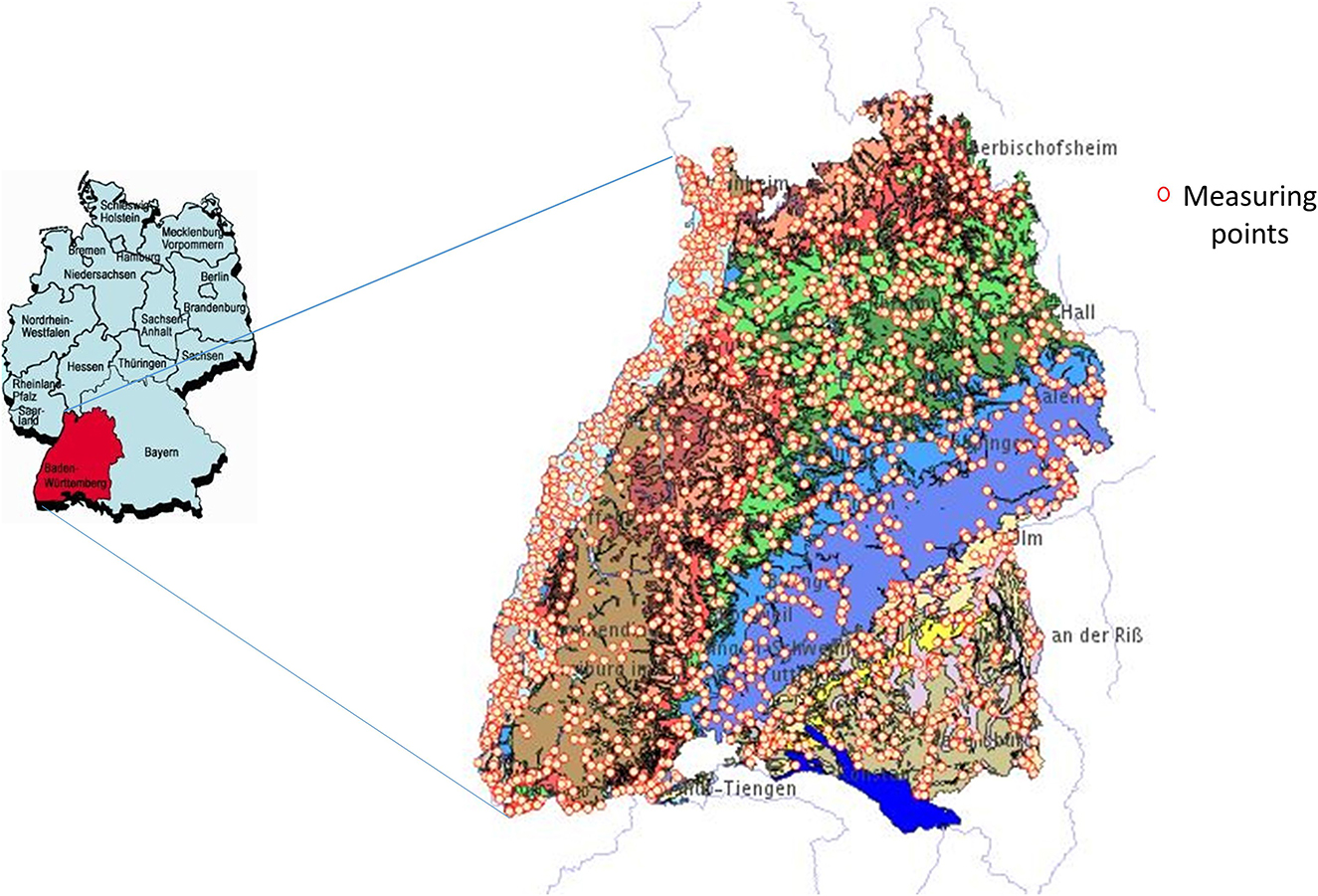
Figure 1. The study area of Baden-Württemberg (BaWü). Generalized hydrogeological map of Baden-Württemberg, southwest Germany, showing karst aquifer systems and locations (Source: Goldscheider and Goeppert, 2009).

There have been some studies about spatial nitrate prediction in the region by the LUBW in 2016, and hence, the results of the 2016 groundwater monitoring programme of the Landesanstalt für Umwelt Baden-Württemberg (LUBW) will serve as a comparison of our methods. The LUBW investigated 1,755 monitoring sites in 2016. The regionalization was done with 1,697 sites using the method SIMCOP-BW (based on copulas; Bárdossy and Li, 2008). The study showed that nitrate concentration shows high spatial variability, and the SIMCOP-BW method was not able to represent small spatial differences.

In order to understand the rationale for the selection of the predictor variables used in the models, a brief introduction to groundwater nitrate and relevant processes is given in the following: Nitrate contamination of groundwater bodies is a common problem in Germany. Nitrogen is essential for plants, which is why mineral fertilizers based on potassium, calcium, sodium, or ammonium nitrate from agriculture are usually the main source of nitrogen surpluses in the underground. Precipitation (atmospheric nitrogen deposition) is another important nitrogen source that includes both anthropogenic and natural components (e.g., Galloway et al., 2008). It is also the primary driving force for nitrate leaching in soil and transport through the vadose zone into groundwater, where complex attenuation processes occur. Aquifer and soil properties and biochemical conditions determine nitrate transport in the direction of groundwater flow and important nitrate removal processes such as denitrification, which occurs only under anaerobic conditions and when denitrifying bacteria as well as reducing agents are present (Rivett et al., 2008). Especially highly productive sedimentary aquifers often show initially high availability but limited amounts of such reactive material; hence, the nitrate removal potential of such aquifers over time is strongly limited. A solid estimation of the nitrate concentration is ideally based on data and proxies that describe all of these factors, such as land use patterns, fertilizer data, weather and climate conditions, topography, groundwater levels, underground properties (depth to groundwater, hydraulic conductivity, effective porosity, etc.), and biochemical conditions (pH, temperature, oxygen (O2) concentration, iron (Fe), organic content, etc.). However, some of these data are either unknown or unavailable, which is especially a problem in the case of data on fertilizer application, presumably the main source of nitrate input. Other important data (e.g., biochemical conditions) are only pointwise measurements without the potential for solid regionalization to use them as spatial predictor variables.

Based on this background, the predictors and the data used for the studies are summarized in Table 1. The nitrate concentration data was taken from the LUBW annual groundwater data catalog and measured from 1,566 monitoring wells in the upper aquifer. The most recent measured values from the years 2016 to 2019 were used for the study. Table 1 shows the data type, the resolution of the data, and its source. The main source of the data was the Federal Institute for Geosciences and Natural Resources (BGR) in Hanover and the German Federal Agency for Cartography and Geodesy (BKG). This provided most of the hydrogeological data, such as hydrological units, soil units, surface geology, etc.

TABLE 1

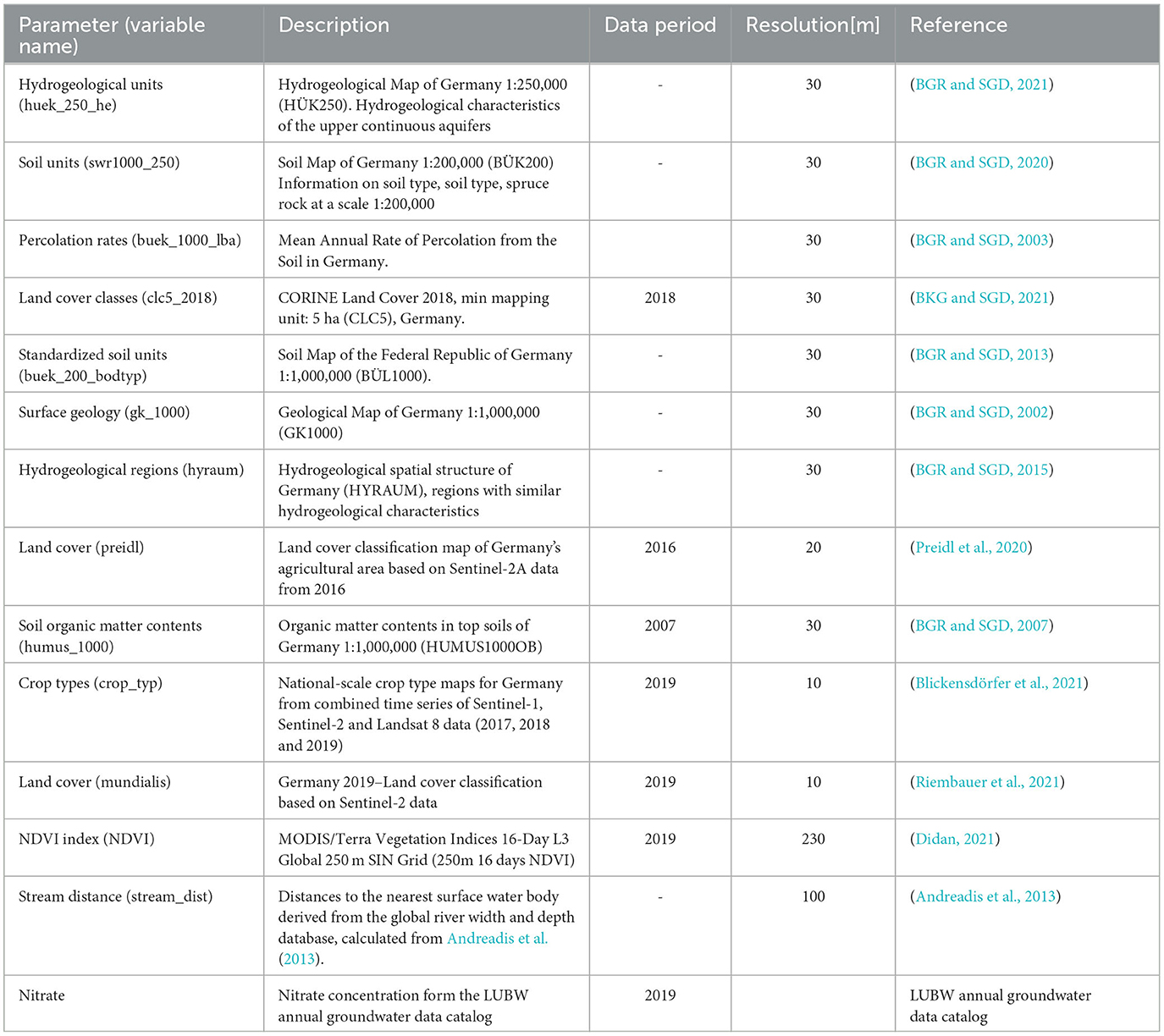
Table 1. Summary of the data used as predictor variables and nitrate concentration as response variable.

Land use and cover are the principle sources of groundwater contamination with nitrates. Especially the information on nitrogen fertilizer load is not directly available, but it is closely related to land use. Farms, industries, and animal distribution statistics are very important covariates that can explain nitrate sources. The CORINE Land Cover (Copernicus Land Monitoring Service) Dataset was applied for this purpose. Furthermore, to improve the data, it was combined with the land use maps from Preidl et al. (2020) and data from Sentinel 2 (Riembauer et al., 2021). The crop type data, which indicates the amount of nitrate fertilizer required, was derived from national scale crop type map for Germany based on a combined time series of sentinel-1, sentinel-2, and Landsat 8 data (2017, 2018 and 2019) (Blickensdörfer et al., 2021). Moreover, NDVI data were used to account for more information on vegetation state. The geological unit, aquifer, and soil type determine how fast the nitrates can be transported through them. Together with the percolation rate, which is determined by precipitation, evaporation and surface conditions, they are primary covariates that influence how fast nitrate is transported into the ground from the surface. Furthermore, the organic matter content of the soil is also used as an explanatory variable to account for biochemical reaction processes in the soil. Another important variable is the distance to the nearest surface water body, which can influence groundwater quality through surface water–groundwater exchange. This data was derived from the global river width and depth database, Andreadis et al. (2013). The list is the result of a broader screening of variables, based on possible influence on groundwater nitrate (from our conceptual understanding of the relevant processes), availability, as well as some preliminary tests. Data, which were originally in vector format, were rastered in a 30 m resolution. For the CNN models, where a common grid of the same resolution and origin is required, the data were further rastered on a common grid of 100 m.

Some statistics of the groundwater nitrate concentration data collected from 1,566 monitoring sites in the area of study are shown in Figure 2. As indicated by the skew of 1.5, the data distribution is quite imbalanced. Lower values of nitrate are more common compared to the higher values above 50 mg/l, which makes it very difficult for learning methods.

FIGURE 2

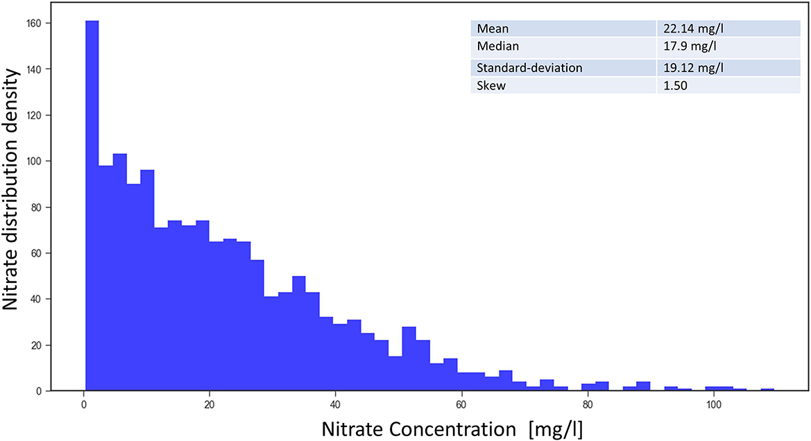
Figure 2. Frequency density of the nitrate concentration from 1,566 measuring sites (mean from 2016 to 2019).

2.2. Methodology

Our methodological approach is shown in Figure 3. Firstly, in step 1—data preprocessing: machine learning data is generated from the raster data by performing a spatial query and encoding (if a categorical variable) the values at the locations of the nitrate observation points. Secondarily, the machine learning models are created, trained, and validated with the data from step 1 using 10-fold cross validation. Optionally, uncertainties are quantified using bootstrapping. Each observation point is evaluated, and the importance of the feature is calculated. Finally, the nitrate concentration is regionalized for the whole model area by iterating over all grid cells of the input variables. All these steps of the methodological approach will be described in detail in the following sections.

FIGURE 3

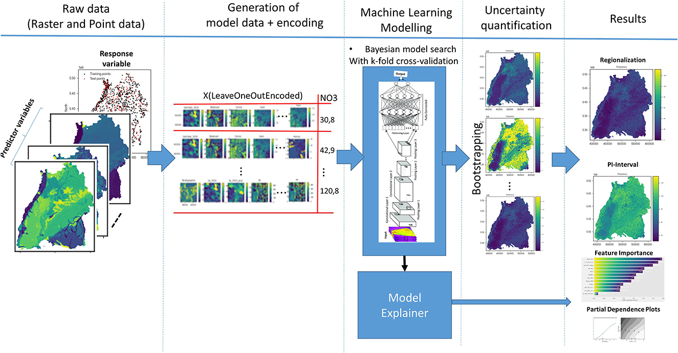
Figure 3. Methodology: from data preparation to regionalization and uncertainty quantification.

2.2.1. Data preprocessing

Both tree-based machine learning methods and CNNs require data for regionalization in a certain format. Data is available in the form of raster files for the predictor variables and as a point shape file for the groundwater nitrate, i.e., the response variable. The first step was data preprocessing and preparation according to the requirements of each machine learning method (tree-based or image-based, i.e., CNN). The interquartile range (IQR) method was applied to the response variable to remove outliers with values of 1.5 times the IQR above the 75% quartile.

In practice, a single groundwater observation well is usually described as a point with coordinates (x, y) and the corresponding nitrate value. Other data are represented by a vector of pixel values from multiple covariate raster images at the same location. For the tree-based methods, the usual approach is that the raster maps of the covariates are stacked together and the values at x and y are extracted for each covariate. Although accurately representing an observation with a point can be beneficial, it does not take into account surrounding information, which can be useful, e.g., to account for transport processes or spatial uncertainties in the input data. Some authors use a simple approximation by taking a buffer around the observation well and taking the mean or majority of all the raster values in the buffer, e.g., Knoll et al. (2019). We tested this approach with different buffer sizes for the random forest model, but without any significant improvement in the results.

In this paper, we first perform feature engineering to encode the spatial position, whereby raster images for coordinate grids X and Y (see Figure 4A), distances to corner and center coordinates of the raster extent, are generated and added to the stack of the covariates (see Figure 4B). Finally, the stack is intersected to get the common pixels, where data is available for all raster images. Next, raster values are extracted at the training point locations to create machine learning data. The random forest model directly utilizes this data for training.

FIGURE 4

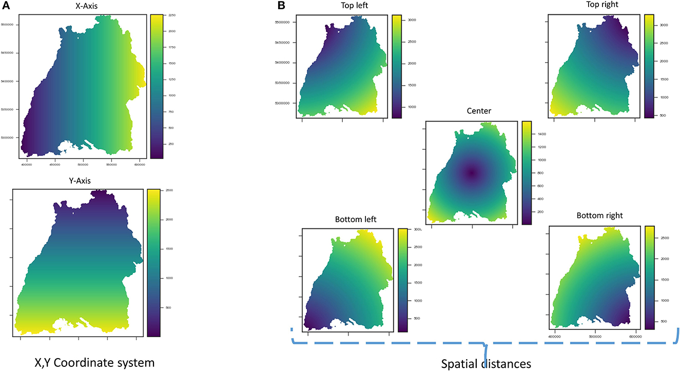
Figure 4. Engineered features (A) coordinate grids X and Y, (B) euclidean distances.

For the CNNs, a more realistic and different approach is taken to include spatial context. CNNs work on images, hence they automatically include information about the vicinity of (x,y) and fully leverage the spatial context of a nitrate observation. The vector of covariates (A_n) is replaced in this case by a 3D array with dimension (h × w × n), where w and h are the width and height in pixels of a window centered at point (P), as shown in Figure 5A.

FIGURE 5

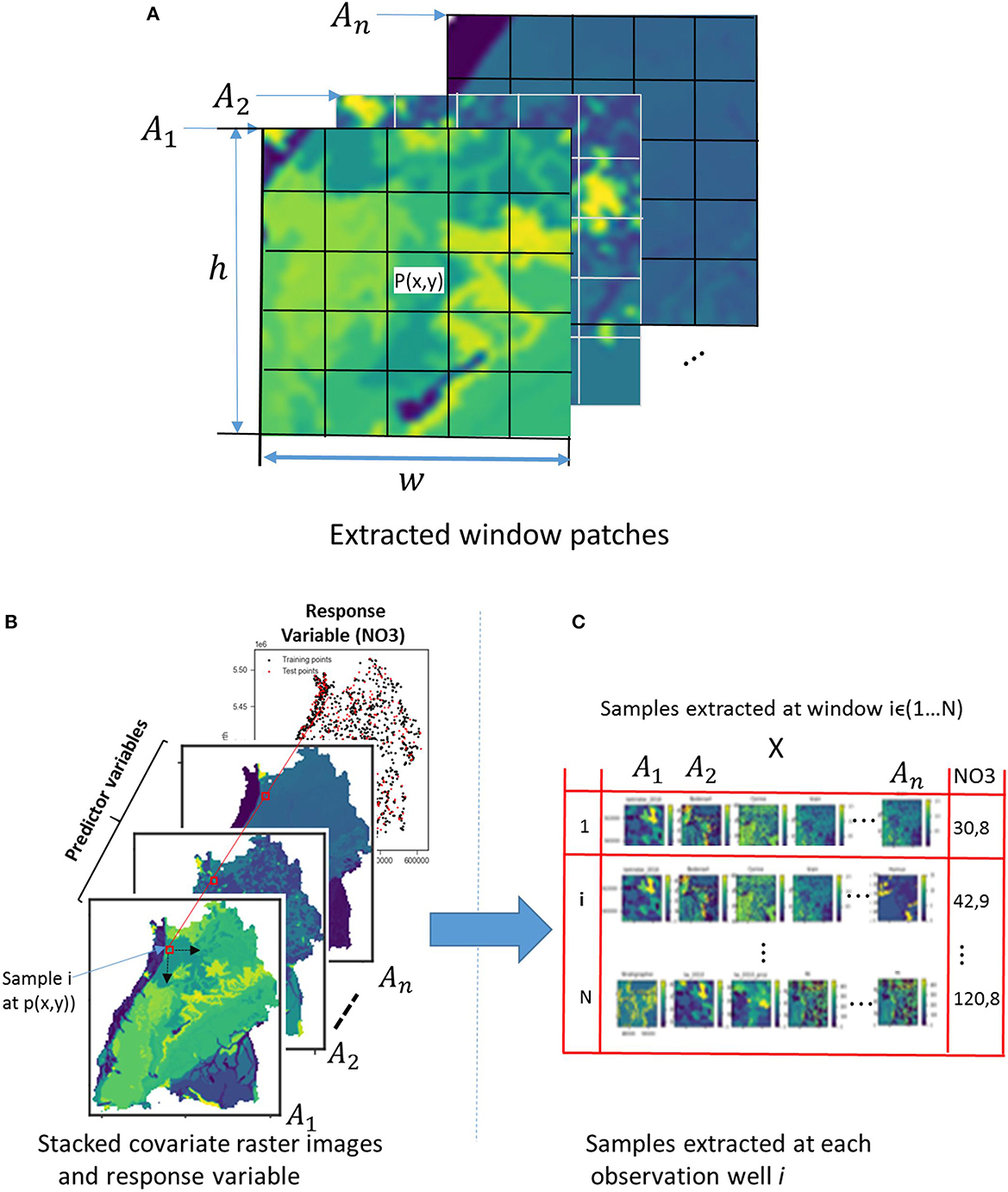
Figure 5. (A) Spatial context in the vicinity of a nitrate observation well (P) for n number of explanatory raster variables. (B) Crops of raster images at the observation wells by a window of size h × w and (C) cropped images representing n different input variables at the same point marked by the red square.

Without a doubt, the area of the covariates influencing the occurrence of nitrate has a limited extent. Finding this hypothetical zone of effect is therefore crucial. This would in turn considerably reduce the size of the inputs supplied to the CNN model as well as the training time. There are many ways of finding the zone of influence, e.g., variogramming and spatial correlation analysis, as illustrated in Padarian et al. (2019). In this paper, the size of the window for cropping the explanatory raster images is estimated in two steps: first, using a variogram to find a rough estimate, and then setting different window sizes around the rough estimate as model hyperparameters and testing their effects on the prediction results using Bayesian optimization to get the best window size. Such a variogram shows the correlation between two spatial data points over distance, i.e., it is a function of variance over distance. The variogram included the averaged variability from all the covariates in order to calculate the zone that best correlates with the response data. Therefore, for the spatial model, the original raster files of the covariates are cropped according to the zone around the observation point, as illustrated in Figure 5B, and put together along with the response variable to make a sample (Figure 5C). In this way, a dataset containing an array of cropped explanatory raster images with their corresponding response values is obtained. If we want to utilize all the observation points available, we will run into a problem at the borders with the points that are less than half the zone distance from the edges. Therefore, all the points that fulfilled this condition are removed from the dataset.

2.2.2. Encoding categorical predictor variables

Most images of the raster variables applied, e.g., for land cover, hydrogeological unit or soil type are categorical and therefore require encoding. Three types of encoders (label, target, and leave-one-out) are implemented and tested. Firstly, the categorical predictors are label encoded, as that is the obvious encoding technique for images. The authors are aware of the limitations of label encoding, which can cause bias in the data since it uses number sequencing. Therefore, for the pilot region and the available data, some tests to see the effect of label encoding were conducted. Ten datasets are formed in which the number sequencing for the encoding was randomized. The tests showed that, for this specific data, there was no significant difference in the results of the prediction observed.

The second and third encoding techniques used were simple target encoding and leave-one-out-encoding, which is another type of target encoder. This type of encoder computes the mean target ${\hat{x}}_{i}^{k}$ of category k of an observation i as with the naive target encoder, but the difference is that the observation j is removed from the dataset as follows:

\begin{array}{l} {\hat{x}}_{i}^{k} = \frac{\sum_{j \neq i} (y_{j} = (x_{j} = = k)) - y_{i}}{\sum_{j \neq i} x_{j} = = k} & (1) \end{array}

This can be easily realized by the following calculations. The mean of a category is computed with:

\begin{array}{l} v = \frac{1}{N_{c}} \sum_{j \in C} y_{j} & (2) \end{array}

where v is the target-encoded value for all samples having category C, N_C is the number of samples having category C, and j ∈ C indicates all the samples which have category C.

Based on the leave-one-out target encoding, the count of samples having category C (N_C) is computed, and then the sum of the target values of those categories are computed separately:

\begin{array}{l} S_{c} = \sum_{j \in C} y_{j} & (3) \end{array}

Then, the mean target value for samples having category C, excluding the effect of sample i, can be computed with

\begin{array}{l} v_{i} = \frac{S_{C} - y_{i}}{N_{C} - 1} & (4) \end{array}

By using a leave-one-out scheme, target data leakage is also prevented. The centers p(x, y) of the extracted patches of categorical variables are aligned with their target values and used for encoding in convolutional neural network data. A comparison of the label and the leave-one-out encoding techniques showed that the leave-one-out encoding performed better and was more reliable in this case. The advantage of the leave-one-out encoding in this case is that it helps to learn useful variations of the data instead of just splitting it by large categorical variables and ensures that every row of data in the dataset becomes related to the response variable after the encoding. This is not the case with the original categorical variable, which may be related to the output only in an indirect, latent manner. Furthermore, the interactions between the predictor variables and the response variable are by definition represented too.

2.2.3. Random forest model

The tree-based model was based on the random forest algorithm designed by Leo Breiman, which combines the results of several decision trees (Breiman, 2001). The random forest is an extremely random tree regressor, which is different from standard decision trees (DTs) in the way they are built. When looking for the best split to separate the samples of a node into two groups, random splits are drawn for each of the randomly selected features, and the best split among those is chosen. According to the data structure described in the data processing section, the RF model was realized according to how the spatial information was incorporated. Coordinate grids as engineered features were generated and added to the raster stack. The RF was implemented and optimized in Python using Bayesian Optimization (Pedregosa et al., 2011). A grid of hyperparameter ranges was defined, a random sample was taken from the grid, and a K-Fold CV was performed with each combination of values. The random forest model's parameters (max_depth, max_features, min_samples_leaf, min_samples_split, and n_estimators) were tuned during cross validation.

2.2.4. Convolutional neural network based models

It is very important to find an appropriate way of fusing heterogeneous information to obtain an optimal response using CNNs. In literature, there are several ways of combining such information using CNNs: unimodal (LeCun et al., 2015; Tran et al., 2015); and fusion networks (Baltrusaitis et al., 2019; Zeng et al., 2019). Both exhibit different performances for different tasks. Therefore, in our work, we implemented the unimodal and fusion architectures, extended them for multi-task learning, and tested them for our groundwater nitrate prediction. The final structure and hyperparameters of the CNNs are obtained using Bayesian optimization (BayesOpt) (Fernando et al., 2014). Convolutional neural networks must have their architecture specified in order to be trained. Options for the training process include learning rate, window size, and L2 regularization strength. It can be highly challenging and time-consuming to choose and tune hyperparameters. A good approach for improving the hyperparameters of deep learning-based regression models is Bayesian optimization (Fernando et al., 2014). The advantage of Bayesian optimization is that it can be used to optimize non-differentiable, discontinuous, and time-consuming functions. Besides the specification of the neural network architecture and deciding the options of the training algorithm, Bayesian optimization is also used to select the most important predictor variables.

The first two CNN architectures are unimodal networks based on 2D (Bengio and Lecun, 1997) or 3D convolution (Tran et al., 2015) have the structure as shown in Figure 6. Hereafter, they will be called 2DCNN and 3DCNN, respectively. In a unimodal network such as 2DCNN or 3DCNN, there is no fusion at all, the inputs are stacked together to form a multi-channel image. We stacked our input raster images into channels to create a h × w×(n Channels) input structure, which goes into the common layers. These initial common layers are there to extract features that are common to all the target depth ranges for nitrate prediction. For the common layers, nfilters₁@3x3 filters were applied with no padding and a stride of 1 in the first convolutional layer with ReLu activation. As in most networks, this was followed by a 2x2 max-pooling layer with a stride of 2 and a dropout layer of dropout rate dropout_rate. This is again fed into the second convolutional layer where nfilters₂@3x3 are used. Next the outputs of the second convolutional layer are led through individual depth branches, flattened to a 1-D array and fed to three fully connected ReLU layers with n_nodes neurons each. Finally, outputs are connected to a fully connected layer of size 1 with a linear activation function, which are consequently the final prediction for the individual target depths.

FIGURE 6

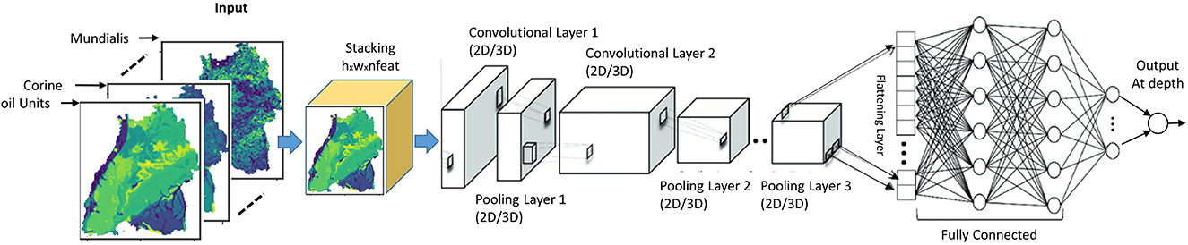
Figure 6. Unimodal CNN architectures for predicting groundwater nitrate concentration based on either 2D or 3D convolution.

In fusion networks, the different modalities run in different stream, and the results are aggregated in some way (Figures 7A, B). Depending on where the fusion takes place, they are named early (Figure 7A), intermediate or late fusion (Figure 7B). In late fusion, there is a unimodal network for every explanatory variable and at the end, the results are combined using some form of aggregation strategy, e.g., summation, weighted averaging and voting. This has some advantages that one can use some sophisticated classifiers for each modality, as well as the use of simple pooling operators and attention mechanisms (Valada et al., 2020) to combine the prediction scores of each stream. This is very practical, that is why the late fusion is used predominantly (Simonyan and Zisserman, 2014). The disadvantage is that you might not take advantages of correlation which might exists between the covariates variables. This architecture of late fusion starts with multi-streaming for the individual channels. For each stream, the common layers of the different depths start like in the previous network with a 2D convolutional layer with nfilters₁@3x3 filters with stride of 1, followed by a 2x2 max-pooling layer with of stride 2 and a dropout layer of dropout rate droput_rate. This is again fed into the second 2D convolutional layer where nfilters₂@3x3 filters are used. After the second convolutional layer, a fully connected ReLu layer with n_nodes neurons is added to each stream, led through individual depth branches, flattened to a 1-D array and fed to three fully connected ReLU layers. Finally, outputs are connected to a fully connected layer of size 1 with a linear activation function, which corresponds to the final prediction for each target depth. The late fusion model will hereafter be called 2DCNN-LF.

FIGURE 7

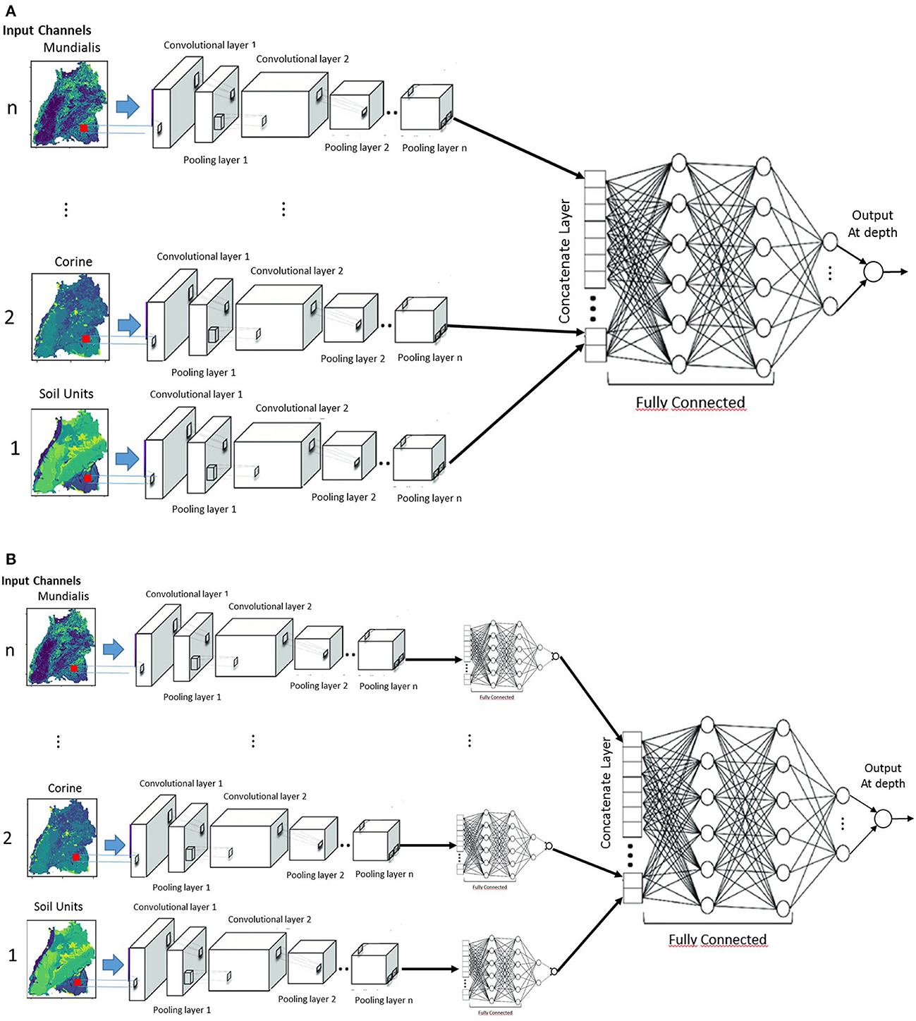
Figure 7. CNN Fusion networks (A) early fusion and (B) late fusion.

If one needs to take advantages of the correlations between the explanatory variables, it is required to process them together, and here we come to early fusion concept (Sun et al., 2017). Each modality is considered independently in the extraction of features. The disadvantage here is that the input modalities need to be synchronized so that they can be processed together. For this architecture, the individual raster images are fed in as M image inputs and each input is fed into its own 2D convolutional layer with nfilter₁@3x3 filters having a stride of 1. The convolutional layer, as in the previous architecture, is followed by a 2x2 max-pooling layer with of stride 2 and a dropout layer of dropout rate dropout_rate. This is again fed into the second convolutional layer, where nfilter₂@3x3 are used. The outputs of the second 2D convolutional layer are then flattened, concatenated, and fed to the independent branches with three fully connected ReLU layers. Finally, for each branch, outputs are connected to a fully connected layer of size 1 with a linear activation function, which corresponds to the final prediction for each target depth. The early fusion model will hereafter be called 2DCNN-EF.

For all models, the Adam optimizer is used for training. Aside from the parameters number of filters (nfilter_x), dropout_rate,window_size, the learning rate was also set as a hyperparameter to be determined by the Bayesian algorithm during cross validation for each model.

2.2.5. Model explanation

For environmental managers, water authorities and water suppliers, it is of practical relevance to know the relationships between the covariates and the model predictions so that they are able to set up measures for improving the groundwater quality. To provide a better understanding of the data and model predictions, feature importance learning and partial dependence analysis of the models were performed in this paper. Feature importance provides a technique to find the best subset of input features by assigning scores to input features on the basis of their contributions in predicting a response variable. Redundancy in machine learning models causes inefficiency in training and introduces unnecessary noise to the models. For the RF model, feature importance is provided as a model result, and for the CNN models, Bayesian model selection was applied, whereby the features were provided as a variable to be optimized. Partial dependence analysis is a technique that provides insights into the marginal effect that one or two input features have on the predictions. By plotting partial dependences, the relationship between the response variable and an input feature can be shown, whether it is linear, monotonic, or more complex in nature.

2.2.6. Uncertainty analysis

The dataset is based on the mean values over a long period of time; hence there are several outliers which can influence the conditional mean. To have useful model skill and reliable results, prediction intervals (PI) should be derived to determine the model uncertainty. PI is defined based on p-quantiles as the interval from the lower ( $P I_{L} = \frac{1 - p}{2}$ ) to the upper limit $P I_{u} = \frac{1 + p}{2}$ ) of the predictions, in which the true value is expected with a high probability (p). For the models RF, 2DCNN, 3DCNN, 2DCNN-EF, and 2DCNN-LF, the uncertainty is presented as p=0.10 prediction interval from several bootstrapping runs. The upper and the lower bounds (PI_L) of the confidence band is computed as

\begin{array}{l} P I_{L} = \bar{x} \pm 1.645 \sqrt{σ^{2} + M S E} . & (5) \end{array}

$\bar{x}$ is the mean and σ²is the variance of the N-bootstrap runs, and MSE is the mean squared error of the fitted models. The bootstrapping procedure follows two steps: 1) computing a population of statistics e.g., mean squared error and then 2) calculating the confidence interval. A population of statistics is created by running the Bayesian optimization for hyperparameter search 100 times. Each time a new model with different hyperparameters is found and its metrics (MSE and variance) calculated. In the second step, the confidence interval is calculated using the resulting statistics.

Several statistical measures such as the mean prediction interval width (MPIW) in Equation 6 and the prediction interval coverage probability (PICP) in Equation 7 can be used to evaluate the uncertainty of the model (Rahmati et al., 2019). The PICP for p gives the proportion of observed values (y_i) within the estimated PI (Dogulu et al., 2015).

\begin{array}{l} M P I W = \frac{1}{n} \sum_{i = 1}^{n} (P I_{i}^{u} - P I_{i}^{l}) & (6) \end{array}

\begin{array}{l} P I C P = \frac{1}{n} \sum_{i = 1}^{n} C, w h e r e C = {\begin{matrix} \begin{matrix} 1 & & (P I_{i}^{u} > y_{i} > P I_{i}^{l}) \end{matrix} \\ \begin{matrix} 0 & & o t h e r w i s e \end{matrix} \end{matrix} & (7) \end{array}

2.3. Experiments and performance evaluation

For the experiments, the models are implemented in Python 3.10 (Van Rossum and Drake Jr, 1995) with Kera (Chollet, 2015) and Tensorflow v2.0 (Abadi et al., 2016). A CPU computer was used for both training and inference. The five models (RF, 2DCNN, 3DCNN, 2DCNN-EF, and 2DCNN-LF) are trained, validated and tested using known nitrate concentrations at monitoring sites. The latest available measured values at the monitoring sites of the period from 2016 to 2019 are used for this purpose. Firstly, all the nitrate data is cleaned removing outliers, and then preprocessed as described in Section 2.2.1 for RF and CNN conformity. The categorical variables are target encoded using the leave-one-out-encoder as described in Section 2.2.3.

For the random forest model (RF), Bayesian optimization with cross validation is applied for hyperparameter search, and the following parameters are found: max_depth = 70, min_samples_leaf = 4, min_samples_split = 10, and n_estimators = 100.

Bayesian optimization is also used for tuning and selection of the hyperparameters of the CNN models (2DCNN, 3DCNN, 2DCNN-EF, and 2DCNN-LF). 10-fold cross-validation is used during the Bayesian optimization, where the data is randomly partitioned into 10 subsets. The model fitted to the remaining 9 subsets is then validated using each subset in turn. In this way, models with better generalizability could be established. Several runs per model could be executed to produce an ensemble of models (every run produces a different parameter combination). In the following assessments, the best ensemble member of each model type is selected for comparison. In the real-world application, the ensemble members are aggregated to get a median spatial prediction to consider model uncertainty. For each CNN model type, the optimization parameters included the window size, input features, batch size, learning rate, number of nodes in the layers, and the number of layers.

To evaluate the performance of the various models, a consistent comparison scheme is required. A good comparison objective is one that represents the average prediction error of the models in terms of unit nitrate concentration. The most commonly used metrics to express this are the mean absolute error (MAE) equation 8, the mean squared error (MSE) equation 9, the coefficient of determination (R2) equation 10, the standard deviation (stddev) equation 11, and the model bias equation 15. The MAE gives a very good idea of the prediction accuracy, but it does not show whether or not the model tends to overestimate or underestimate the predictions. This is where the bias comes into play. It allows for the evaluation of prediction accuracy as well as whether the model tends to overestimate or underestimate the values of the variable of interest. The better the prediction, the closer the bias is to zero. It should be noted that the bias does not account for the variability of the predictions. On this issue, a useful metric is the MSE. It provides an indication regarding the dispersion or variability of the prediction accuracy. Therefore, these metrics were used in combination to evaluate the performance in terms of accuracy of the models in this paper.

\begin{array}{l} M A E = \frac{\sum_{i = 1}^{n} | {\hat{y}}_{i} - y_{i} |}{n}, & (8) \end{array}

\begin{array}{l} M S E = \frac{\sum_{i = 1}^{n} {({\hat{y}}_{i} - y_{i})}^{2}}{n}, & (9) \end{array}

\begin{array}{l} R^{2} = 1 - \frac{\sum_{i = 1}^{n} {(y_{i} - {\hat{y}}_{i})}^{2}}{\sum_{i = 1}^{n} {(y_{i} - {\bar{y}}_{i})}^{2}}, & (10) \end{array}

\begin{array}{l} B i a s = \frac{\sum_{i = 1}^{n} ({\hat{y}}_{i} - y_{i})}{n}, & (11) \end{array}

where n is the number of observations, y_i is the value of the ith observation in the validation/test dataset, ${\bar{y}}_{i}$ is the mean value of the validation/test dataset and ŷ_i is the predicted value for the ith observation.

The quality of the PIs produced by the models were evaluated using the mean prediction interval width (MPIW) and the prediction interval coverage probability (PICP). These metrics were described in Section 2.2.5 by equations 6 and 7, respectively. The R² gives us the proportion of the variance in the dependent variable that is predictable from the independent variables and indicates the covariance in the model's prediction. The bias is an indicator for the average difference between the measured and predicted groundwater nitrate values, and the variance gives the degree of spread of the predictions.

3. Results

The models were evaluated on their performance based on six metrics (MAE, STDdev, R², Bias, and where appropriate, PICP and MPIW) after the Bayesian optimization with 10-fold cross validation, and the results are shown in Table 2. The training and inference times of the different models are also listed in the table as a proxy for complexity of the model.

TABLE 2

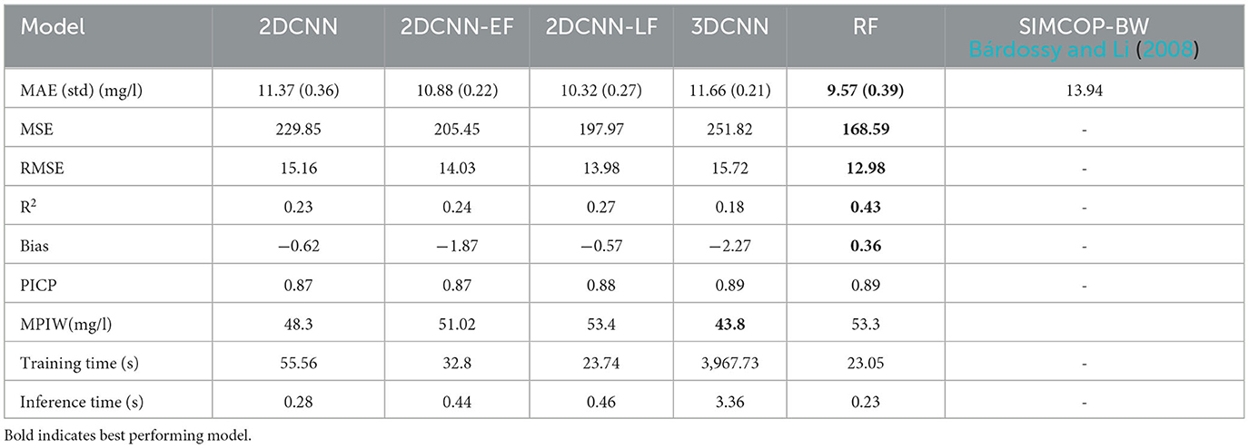
Table 2. Validation results of own the models compared to the results of a previous study of the LUBW in Bárdossy and Li (2008) of the model SIMCOP-BW.

The RF best performed with MAE of 9.57 mg/l. The 2DCNN-LF had the best MAE of all CNN models with 10.32 mg/l and standard deviation of 0.27 mg/l. The other models 2DCNN-EF, 2DCNN and 3DCNN were also in the same performance region with 10.67 mg/l, 11.37 mg/l and 11.66 mg/l, respectively. In terms of R², the RF model with 0.43 outperformed the best CNN model with 0.27 significantly. This can be due to the fact that the resolution of the common grid of the input rasters for the CNN was quite large with 100 m. The difference between the 2DCNN and the 3DCNN can be explained by the fact that even though the 3DCNN has an extra dimension that enables the convolution with the filters input-wise, unlike element-wise in the 2DCNN, and can transport the nonlinear information better, it adds unnecessary tunable parameters that make it more difficult to define the model structure. The difference between the early fusion model 2DCNN-EF and the late fusion model 2DCNN-LF shows us that the non-linear interactions between the inputs play a very big role because the early fusion focuses more on the more complex interaction between the covariates and the late fusion focuses more on the feature extraction from the covariates. The time differences for training and inferring the different models are in alignment with their complexity, which is arranged in descending order as follows: 3DCNN, 2DCNN, 2DCNN-EF, 2DCNN-LF, and RF. High uncertainties in the models are confirmed by the mean predictive interval width (MPIW) in the range of 43–54 mg/l in all the models. The prediction interval coverage probability (PICP) of 0.87–0.89 for the nitrate concentration correspond to α = 0.10, which is a very good indication that the uncertainty assessment using bootstrapping was successful. Similar studies on estimation of groundwater nitrate concentration, e.g., in Ransom et al. (2017), Knoll et al. (2019), Koch et al. (2019), Rahmati et al. (2019) show similar uncertainty results.

Scatterplots of the nitrate predictions by the models are shown in Figures 8A–E. Scatterplots provide insight into the degree of fitness of the models, the model bias, and the variance of predictions shown in Table 2. The clouds of all the models' predictions show scatter, particularly in the high values, which is consistent with the positive and negative biases of the models with the 2DCNN-LF and the RF models having the lowest biases of −0.57 mg/l and 0.36 mg/l, respectively (Table 2). The 3DCNN model has less scatter in the predictions compared with the other model (Figure 8B), which is expressed by the slightly lower prediction variance of 0.21 mg/l (Table 2).

FIGURE 8

Figure 8. Measured vs. predicted groundwater nitrate concentrations for (A) RF, (B) 2DCNN, (C) 3DCNN (D) 2DCNN-EF, and (E) 2DCNN-LF models. The red line represents the ideal predictions and the blue lines, the regression line of the point cloud.

After training, the models were used to predict the nitrate concentration for the whole grid, including unknown regions. For the CNN-based methods, a sliding window of the size determined by the Bayesian optimization algorithm is run through all the raster cells to produce a target dataset, with each sample containing the N explanatory raster. In this way, a map of nitrate prediction can be produced.

The regionalization results of the CNN models, and RF model are shown as raster maps in Figures 9A–E. Please note the difference maximal values of the color bars. It can be seen that all the methods produce similar, plausible results for regionalization (with slight differences), which is in accordance with results of former studies as well as correspond to our conceptual understanding. If the sampling locations are overlaid on the prediction surface, the spatial pattern of the observed nitrate concentration concurs very well with the predictions (data not shown). Higher nitrate concentrations are identified in the northern region, where most of the agricultural activities are conducted, and in some regions with porous aquifers. The lowest groundwater nitrate concentration is identified appropriately in the regions with karstified aquitards, e.g., in the Black Forest region, where fewer human influences such as agricultural activities are occurring. High nitrate concentrations can also be found in the middle Neckar-Taube-Gäuplatten, near the southern edge of the Black Forest in the northern part of the Swabian Keuper-Lias Plains, in the middle of the Donau-Iller-Platte and the bordering northern part of the Voralpien Huegel and Moorland, in the southern and northern parts of the Oberrhein-Tieflands, and in the north of the Odenwaldes. These areas are also mentioned as having high nitrate concentrations in the LfU report 2001.

FIGURE 9

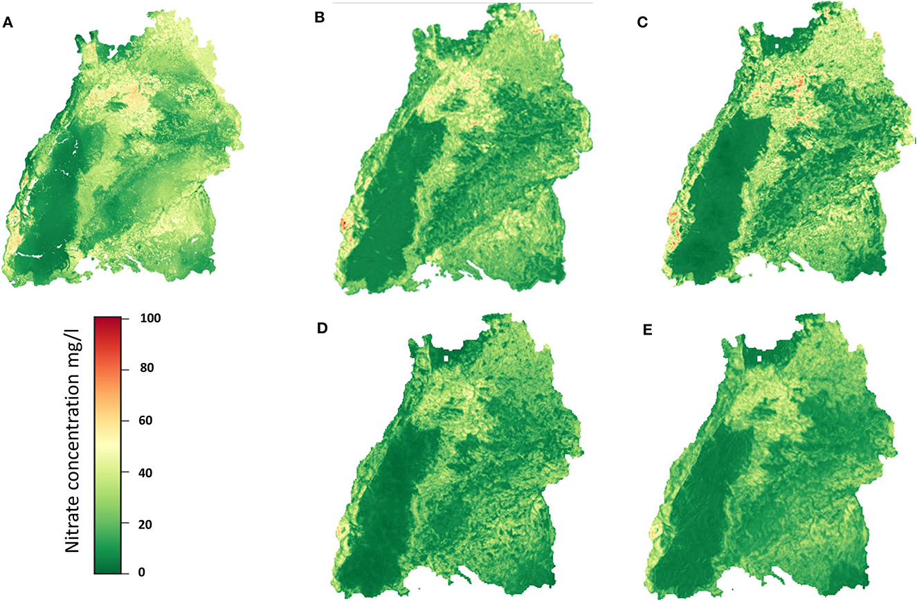
Figure 9. Regionalization results of the (A) RF, (B) 2DCNN, (C) 3DCNN (D) 2DCNN-EF, and (E) 2DCNN-LF models.

Compared to the RF and the SIMCOP-BW (see, Bárdossy and Li, 2008), methods, the CNN models produce uniform regionalization images, as can be seen in Figures 9C–F. In the image of RF (Figure 9A), there are some unnatural artifacts edging the dark green area. The RF, 2DCNN, 3DCNN models get the peaks much better than the fusion networks.

The RF and the 2DCNN models were used for feature analysis using partial dependence of model predictions to the input features. The importance table and the partial dependency plots of the most important variables are shown in Figures 10, 11, respectively. Looking at the importance table in Figure 10, results show that groundwater nitrate concentration is dependent on the combination of several factors, including soil, hydrology, geomorphology, and land cover or use. The results obtained are in alignment with the results of previous studies, e.g., Knoll et al. (2019), Ouedraogo et al. (2019), and Ransom et al. (2022). The models show that the soil units (“buek_200_lba”), soil type (“buek-200-bodtyp”), distance from streams or rivers (“StreamDist”), geology (“gk_1000”), NDVI (“NDVI”), land cover (“clc5_2018”), and land use (“Mundialis”) are the most crucial covariates for the nitrate prediction. Unfortunately, land management data (types of crops and how much fertilizer is used by the farmers) is not available; such features would definitely improve the results significantly.

FIGURE 10

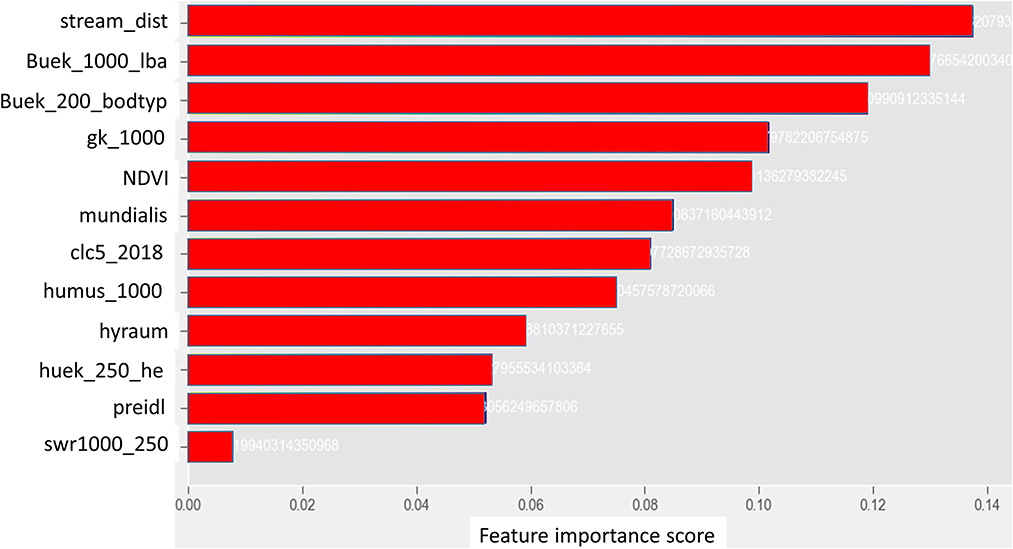
Figure 10. Ranking of the importance of the input features. The names are defined in Table 1.

FIGURE 11

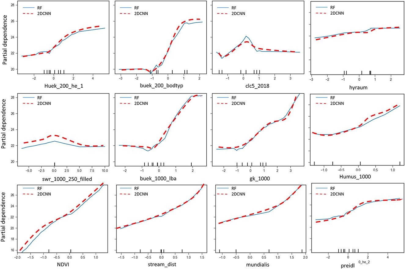
Figure 11. Partial dependence plots of important input variables.

Partial dependence plots (PDP) for all the most important variables are shown in Figure 11. All the models show similar relationships, as can be seen. Low values of “buek-1000-lba,” showing undeveloped land areas like in the region of the Black Forest where there are no fertilizers and manure additions, are associated with lower nitrate concentrations. The nitrate concentration gradually increases from these areas to areas of agricultural use with orchards and vineyards, and then gets even higher in areas of urban use. Therefore, the soil units “buek-1000-lba” have a positive correlation with the groundwater nitrate concentration. A positive correlation can also be seen between “buek-200-bodtyp” and nitrate concentration; poorly drained soils such as clays are associated with low nitrate concentration, while in more sandy areas, nitrate concentration is high while cropping is more intense, like in the edges of the Black Forest in the vineyards. Nitrate concentration is low in areas with fewer anthropogenic effects, as denoted by low values of “clc5-2018” and “Mundialis,” and high in areas of intensive agriculture, which shows a direct dependence of nitrate concentration on land cover and land use. The opposite relationship applies between “NDVI” and nitrate concentration. Low nitrate concentrations are predicted in areas with high “NDVI,” such as the Black Forest, so there is an inverse relationship between NDVI and groundwater nitrate concentration. Even though the percolation rate is not classified as being of high importance, there is a direct positive correlation between the percolation recharge (“swr-1000_250_filled”), humus content (“Humus_1000”), and nitrate concentration. High percolation rates allow for higher nitrate leaching and, therefore, a higher nitrate concentration in the groundwater. Higher humus content in soils is favorable for agricultural activities and therefore associated with higher nitrate from fertilization.

Two-way partial dependence plots for two covariates are illustrated in Figure 12. It is clear that the soil type “buek-200-bodtyp” interacts with the percolation rate “buek_1000_lba,” showing that groundwater nitrate is dependent on the joint influences of the two covariates. The interactions between these two covariates are obvious. Based on the leave-one-out target encoding, for lower values of “buek-200-bodtyp,” i.e., rock and poorly drained soils such as clay, the nitrate concentration is nearly independent of the soil type, whereas with decreasing values, i.e., sandy soils, the relationship becomes stronger and the percolation rate (buek_1000_lba) increases. Another two-way partial dependence plot of the input variable geological units (“gk_1000”) and the percolation rate (“buek-1000-lba”) is illustrated in Figure 12. The nitrate concentration increases when both variables increase, which is in alignment with the leave-one-out target encoding applied here. Both covariates have, for all their values, a consistent direct relationship with predicted nitrate concentration, as can be seen in the single plots in Figure 11. There is no significant evidence that “buek-1000-lba” is interacting with “gk_1000.” The interactions between “gk_1000” (category: unconfined aquifers) and land use with anthropogenic presence, nitrate fertilizers from agriculture, and livestock correlate with high groundwater nitrate, whereas in areas with “gk_1000” (category: impervious layers), there is less nitrate leaching. The plot of the humus “Humus_1000” vs. land use shows the interactions between them. Humus and arable land in land use are positively correlated with nitrate concentration due to fertilization.

FIGURE 12

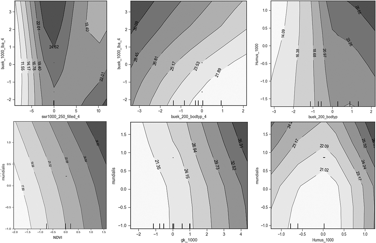
Figure 12. Two-way partial dependence plots of humus, geological surface units, soil type and land cover and land use.

Figure 13 shows a plot of the uncertainty band width of the different models for the regionalization. The plots show the high uncertainty of the predictions, and the comparison between Figures 9, 13 shows the same behavior that the uncertainties increase with the amount of the groundwater nitrate concentration. It can also be seen that the models which perform poor in terms of specific value prediction are the ones which can tolerate uncertainties much better as indicated by the uncertainty band width. In this respect the 3DCNN model (Figure 13C) is more robust and has the least band width.

FIGURE 13

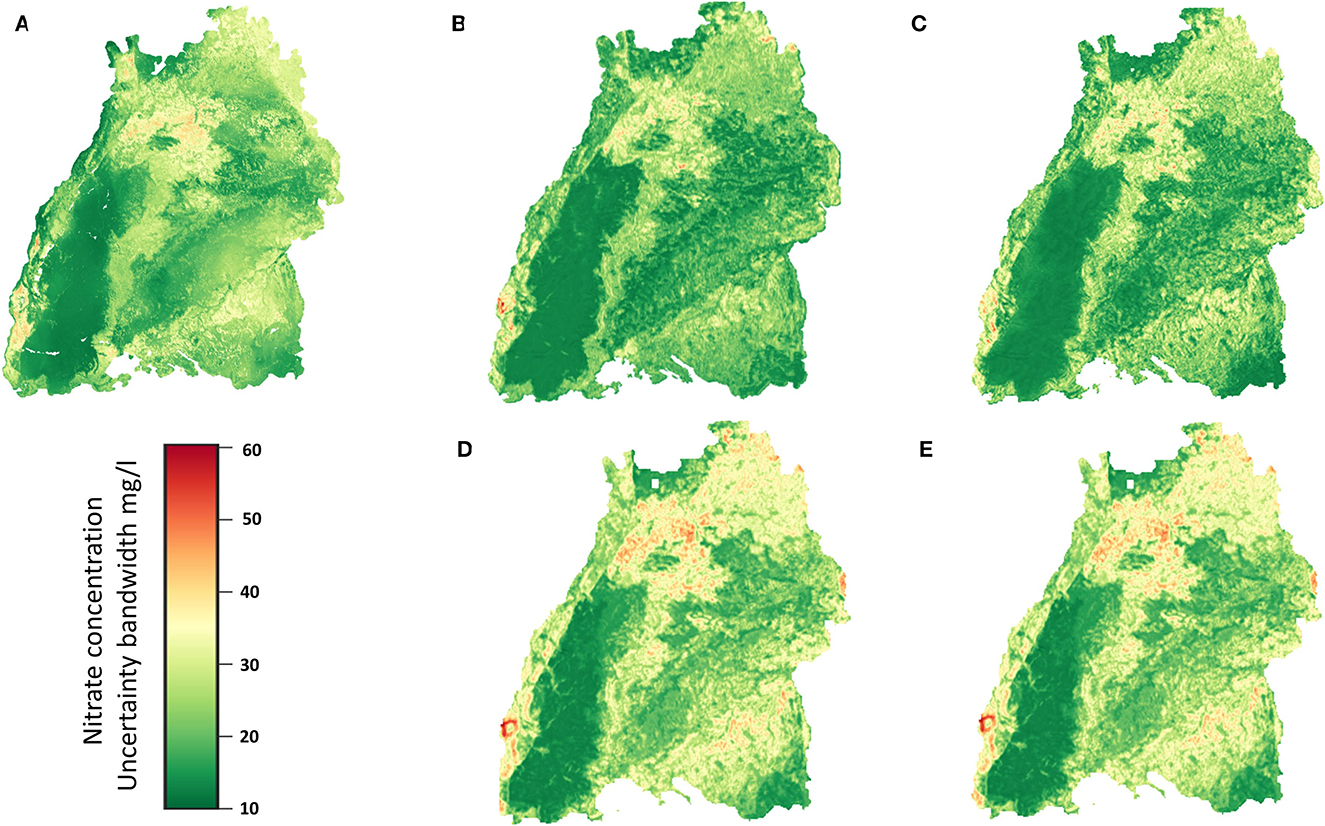
Figure 13. Uncertainty band width for the different models obtained from bootstrapping as described previously. (A) RF, (B) 2DCNN, (C) 3DCNN, (D) 2DCNN-EF and (E) 2DCNN-LF model.

4. Discussion

For comparison and positioning of the results in general, there have been previous studies for regionalization on nitrate in the study area that can be used, and their results are also listed in Table 2. Firstly, the study performed by Bárdossy and Li (2008) with the model SIMCOP-BW shows an MAE of 13.94 mg/l. Our study's models produce significantly better results, with an MAE of <11.70 mg/l by the worst model. However, it must be admitted that the results are not directly comparable, due to the different database [slightly more and partly different model sampling sites and an average higher nitrate values in the study of Bárdossy and Li (2008)]. The studies on uncertainty is in alignment with similar previous studies on estimation of groundwater nitrate concentration, e.g., in Ransom et al. (2017), Knoll et al. (2019), Koch et al. (2019), Rahmati et al. (2019).

The different results of the CNN architectures can be explained by their different data processing mechanisms. The unimodal 2DCNN convolves a M × M kernel with the n-stream inputs to linearly combine the inputs element by element at the first convolutional layer. In this way, no possible nonlinear interactions between the covariates are taken into consideration, and the complete information of the individual streams is not preserved and passed on to the fully connected layers. The 3DCNN deals with this limitation by convolving the filter input-wise due to its extra dimension. Thereby, the information from the different streams is preserved and transported to the fully connected layers. However, the output of its first convolutional layer increases with the number of inputs, which leads to unnecessary tunable parameters in the network and lower data use efficiency. On the other hand, the fusion networks address these two issues of the 2DCNN and 3DCNN networks by convolving the inputs independently with the filters set for each one. When comparing the LF and EF models, it is reasonable to say that LF focuses on better feature extraction from inputs, while EF can model more complex interactions between variables. In addition, by reducing the dimension of each input before combining them, the LF model becomes easier to train, leading to higher data efficiency.

5. Conclusion

In this paper, different types of machine learning models were developed and applied to solve the problem of regionalization of nitrate concentration in groundwater. The models included a random forest model as a baseline model, and several more elaborated CNN models, namely, a 2DCNN, a 3DCNN, a 2DCNN based on an early fusion technique, and a 2DCNN based on a late fusion technique. Spatial information was included in the random forest model by extending the feature inputs with engineered features based on spatial information such as the distance matrix, whereas spatial autocorrelation was included in the CNN models via model immanent characteristics. The input data included spatially continuous information on soil, geology, hydrogeology, and landuse/landcover, as well as plant activity. Most of the predictor variables are categorical, therefore, several encoding techniques were tested for their performance, and the best results were found with the leave-one-out encoding. This was applied to all categorical input raster images.

It could be shown that convolutional neural networks, with their ability to extract spatial features and explicitly take spatial information from explanatory variables around observations, are an intuitive way to perform spatial prediction, even though the random forest model produced comparatively the best result. It was important to show the effectiveness and data efficiency of the different CNN setups (2D/3D convolution, early or late fusion) for groundwater nitrate concentration estimation. Hyperparameter tuning and selection are very difficult tasks for CNNs. Therefore, Bayesian optimization with 10-fold cross-validation was used to automatically find the parameters, which included the features, the window size, and others. The visualization of the spatial variability of groundwater nitrate concentration, the interpretation of the importance of the covariates, and the analysis of the partial dependence plots can provide water and environmental managers with valuable information for understanding local areas that are susceptible and vulnerable to nitrate leaching in terms of land use, land management, and geomorphology. Furthermore, nitrate prediction is associated with uncertainties, as several previous studies have shown. Therefore, all the models were extended to quantify uncertainty using prediction intervals (PIs) using bootstrapping and the results of the models are in alignment with that of similar previous studies. Quantifying uncertainty offers several benefits for water managers, such as the reduction of risk and the ability to plan in a more reliable manner.

The predictive performance of the models was tested on a dataset from a pilot region in Germany, the State of Baden-Württemberg and the results show that, in general, all the machine learning models achieve plausible and good spatial predictive performance compared to the results of a previous study in this region, in which the SIMCOP-BW model (Bárdossy and Li, 2008) was used and produced an MAE of 13.9 mg/l. Based on the mean absolute error, the 2DCNN-LF and the random forest models performed the best with an MAE of 10.32 mg/l and 9.55 mg/l, respectively, and the worst model was the 3DCNN with an MAE of 11.66 mg/l. High model uncertainties were found in groundwater nitrate prediction as measured by the MPIW between 43 and 54 mg/l and PICP between 0.87 and 0.89. This confirms the results from previous studies, e.g., Koch et al. (2019) study that the uncertainties associated with spatial nitrate prediction are large. The different CNN setups (2D/3D convolution, early or late fusion) for groundwater nitrate concentration estimation showed that there are a lot of non-linear interactions between the inputs, as the unimodal and early fusion models, which all focus on the complex relationships between the inputs, performed best among the CNN models. The results of the CNN network comparison cannot be generalized to other application fields because different results exist in other references. For example, fusion networks performed better than unimodal networks in Barbosa et al. (2020) application of the CNN network to soil prediction, and the early fusion strategy performed best in Gadzicki et al. (2020) application. Hence, the decision of which strategy to use unimodal, early fusion, or late fusion should be made application specific.

The quality of machine learning models is largely determined by the quality of the input data. As a result, there is potential for future improvement by using higher resolution raster data, particularly for land use, as well as data that better depict nitrogen fertilizers application more accurately. In this paper, a 2-dimensional regionalization process was performed, but in the future, 3D regionalization will be aspired for when nitrate concentrations are available at different depths. Another limitation of this study is that seasonal changes cannot be assessed. A further study with more focus on spatio-temporal changes in groundwater nitrate prediction is desirable, but up to date fails on the availability of nitrate data with a meaningful temporal resolution. Despite having good performance in specific value prediction, the models described in this paper, produce poor uncertainty estimates. Since overly confident yet incorrect predictions may be harmful, precise uncertainty quantification is integral for practical applications of such networks. To this end, we propose in the next paper a 2DCNN-QD (the 2DCNN uncertainty quality definition), which not only automatically learns complex dependencies between different variables and uses them to regionalize nitrate in unobserved areas but also models the uncertainty of predictions.

Data availability statement

Due to its proprietary nature supporting data cannot be made openly available. Further information about the data and conditions for access are available on request from the authors.

Author contributions

Study conception and design: DK, JW, and TL. Data collection: MO, AW, and TL. Analysis and interpretation of results: DK, AW, and TL. Draft manuscript preparation: DK, LR, and TL. All authors reviewed the results and approved the final version of the manuscript.

Funding

The work is part of the Project NiMo—Nitrate Monitoring 4.0 Intelligent Systems for sustainable reduction of nitrates in groundwater, which was funded by the Federal Ministry for the Environment, Nature Conservation, Nuclear Safety and Consumer Protection.

Acknowledgments

We acknowledge the contributions of all colleagues, institutions, or agencies that aided the efforts of the authors, especially the Landesanstalt für Umwelt Baden-Württemberg (LUBW) for providing us with data on nitrate concentration and agricultural land use information.

Conflict of interest

The authors declare that the research was conducted in the absence of any commercial or financial relationships that could be construed as a potential conflict of interest.

Publisher's note

All claims expressed in this article are solely those of the authors and do not necessarily represent those of their affiliated organizations, or those of the publisher, the editors and the reviewers. Any product that may be evaluated in this article, or claim that may be made by its manufacturer, is not guaranteed or endorsed by the publisher.

References

Abadi, M., Barham, P., Chen, J., Chen, Z., Davis, A., Dean, J., et al. (2016). Tensorflow: a system for large-scale machine learning. In: 12th USENIX Symposium on Operating Systems Design and Implementation (OSDI 16). p. 265–283.