Abstract
In this study, we develop a machine-learning (ML)-enabled strategy for selecting hillslope-scale ecohydrological monitoring sites within snow-dominated mountainous watersheds, with a particular focus on snow-soil–plant interactions. Data layers rely on spatial data layers from both remote sensing and hydrological model simulations. Specifically, a Landsat-based foresummer drought sensitivity index is used to define the dependency of the annual peak plant productivity on the Palmer drought severity index in the early growing season. Hydrological simulations provide the spatiotemporal dynamics of near-surface soil moisture and snow depth. In this framework, a regression analysis identifies the key hydrological variables relevant to the spatial heterogeneity of drought sensitivity. We then apply unsupervised clustering to these key variables, using the Gaussian mixture model, to group hillslopes into several zones that have divergent relationships regarding soil moisture, snow dynamics, and drought sensitivity. Using the datasets collected in the East River Watershed (Crested Butte, Colorado, United States), results show that drought sensitivity is significantly correlated with model-derived soil moisture and snow-free timing over space and time. The relationship is, however, non-linear, such that the correlation decreases above a threshold elevation and in a heavy snow year due to large snowpacks, lateral flow, and soil storage limitations. Clustering is then able to define the zones that have high or low sensitivity to drought, as well as the mid-elevation regions where sensitivity is associated with the topographic aspect and net potential radiation. In addition, the algorithm identifies the most representative hillslopes with road/trail access within each zone for installing monitoring sites. Our method also aims to significantly increase the use of ML and model-simulation results to guide critical zone and watershed monitoring activities.
1 Introduction
Watershed monitoring always raises the same practical questions: “Where should sensors be placed?” “Which hillslope would be most adapted to perform a field experiment or deploy monitoring equipment?” or “Given a particular site, how representative is it of the watershed?” These are all challenging questions for critical zone and watershed sciences (Strachan et al., 2016). Watersheds consist of diverse biotic/abiotic above-/below-ground compartments interacting with each other through hydrological, ecological, geomorphological, and geochemical processes (Sivapalan, 2006; Wagener et al., 2007).
To answer this type of questions, there have been several studies on sensor placement optimization for soil moisture and snow distribution in watershed science (Kerkez et al., 2012; Oroza et al., 2016) and stream flow depths (Zhang et al., 2019). However, they have focused on estimating the spatial distributions of a single or two target variables. A recent pressing issue has been to observe and quantify interacting ecosystem or watershed responses to the disturbances resulting from climate change, such as coupled soil–plant responses to droughts or wildfires (e.g., Sloat et al., 2015; Mirus et al., 2017; Siirila-Woodburn et al., 2021; Newcomer et al., 2023), or to investigate those disturbances’ key modulators, such as subsurface conditions, which are often difficult to characterize over space and time.
There have been significant advances in quantifying the above/below-ground watershed compartments over space based on a suite of remote sensing datasets, including plant species distributions and traits (e.g., Madritch et al., 2014; Falco et al., 2019; Chadwick et al., 2020; Falco et al., 2020), soil thickness and soil properties (e.g., Patton et al., 2018; Yan et al., 2020), and bedrock variability (e.g., Parsekian et al., 2015; Uhlemann et al., 2022). The co-variability of these compartments has been documented based on analyzing multiple remote sensing and spatial data layers (e.g., Wainwright et al., 2015; Pelletier et al., 2018; Devadoss et al., 2020; Hermes et al., 2020; Enguehard et al., 2022; Wainwright et al., 2022a). In addition, dynamic properties (such as snow distribution and plant productivity) can be estimated across the watershed scale using airborne and satellite remote sensing (Painter et al., 2016; Dong et al., 2019).
In parallel, integrated ecohydrological and reactive transport models have been successfully implemented to describe and predict watershed behaviors from hillslope to continental scales (e.g., Bierkens et al., 2015; Carroll et al., 2019; Xu et al., 2022). Coupled three-dimensional surface water and groundwater flow models have been augmented by land models representing plant water uptake and evapotranspiration (e.g., Condon and Maxwell, 2015; Maina et al., 2021). These models can physically predict the water budget and export at the watershed scale. In addition, reactive transport models have been developed at the watershed scale to quantify geochemical processes such as weathering, nutrient cycling, and solute export (e.g., Li et al., 2017; Li, 2019; Maavara et al., 2021; Xu et al., 2022). These models can predict distributed properties such as soil moisture, water table depth, weathering rate, and other properties over space and time.
Despite the availability of spatial data layers, there have been few studies developing a systematic framework to optimize observation locations (including sensor/well locations) or to choose particular hillslopes/catchments to maximize the efficacy of critical zone experiments. In particular, there is a need to take advantage of landscape heterogeneity to identify key controls, capture distinct ecohydro-biogeochemical regimes, and/or test particular hypotheses with sites are properly distributed (e.g., Sloat et al., 2015; Sanders-DeMott et al., 2018). At the same time, a number of restrictions have to be considered, such as protected areas (e.g., private property and wilderness designated), road accessibility, disturbances to recreation, and others.
This study aims to develop an effective strategy for guiding the selection of observation/experiment locations by combining remote-sensing data layers and model simulation results. In particular, we explore how best to locate multiple observation sites across a watershed to investigate underlying mechanisms that dictate the sensitivity or vulnerability of ecosystems to climate disturbances such as droughts. The ecosystem and plant responses can be directly observed by satellite images such as the year-to-year variability of the Normalized Difference Vegetation Index (NDVI; e.g., Knowles et al., 2017, 2018; Dong et al., 2019; Wainwright et al., 2020). The underlying processes, such as soil moisture and groundwater table dynamics, cannot be observed over space, but we may be able to take advantage of model simulations.
We employ a two-step process: (1) regression analysis of satellite-derived ecosystem sensitivity as a function of model-derived hydrological state variables (soil moisture, water table elevation, snow depths, snowmelt timing, and melt rate) to identify key variables for the sensitivity and (2) cluster analysis based on these variables to identify regions that have divergent responses. This work leverages zonation studies by Wainwright et al. (2022a) and Maina et al. (2021). We consider the hillslope as a unit since the critical zone or watershed science studies are often based on the hillslope-scale observations/experiments, which capture the hydrological connectivity from the ridge to the valley.
Here, we study the East River and adjoining three watersheds near Crested Butte, Colorado, United States (Hubbard et al., 2018) as a demonstration site for the approach combining remote sensing and hydrological model data products to identify distinct hillslope zones that exhibit divergent eco-hydrological characteristics. With regard to the ecosystem response, we consider the heterogeneity of the foresummer drought sensitivity based on the Landsat NDVI developed by Wainwright et al. (2020). This drought sensitivity represents the plant productivity responses to early snowmelt and subsequent drought conditions in the early growing season. In addition, we use the hydrological state variables, including soil moisture and snow depth, computed by a hydrological model (Carroll et al., 2022b). The snow-soil–plant interactions have been studied by ground-based monitoring (e.g., Sloat et al., 2015; Sanders-DeMott et al., 2018) and a combination of ground-based and remote-sensing data (e.g., Devadoss et al., 2020; Hermes et al., 2020). We aim to improve our understanding of these interactions—particularly their spatiotemporal variability.
2 Site and datasets
2.1 Study domain
The domain includes four catchments, including the East River, Washington Gulch, Slate River, and Coal Creek. The elevation ranges from 2,800 to 4,000 m (Figure 1A). Within the four watersheds, the three life zones are defined based on the elevation as the montane (2,400–3,000 m; 33%), subalpine (3,000–3,500 m; 52%), and alpine zones (>3,500 m; 15%). In the USGS National Land Cover Database (NLCD 2011) map (Figure 1B), the key land-cover types are rocky outcrop (12%), evergreen forest (29%), deciduous forest (18%), grassland (30%), and woody wetland (6%). Geology within the domain is complex, including Paleozoic and Mesozoic sedimentary rocks (Mancos Shale, Dakota Sandstone) and tertiary igneous laccoliths (Uhlemann et al., 2022). Within the domain, igneous rocks can be mostly seen in the higher elevation zones, while the lower elevation zone is dominated by shale.
Figure 1

Study domain and four watersheds with (A) elevation and (B) land cover map (USGS NLCD 2011). The red box is the SNOTEL site, the dashed black lines represent trails, and the white lines represent streams and rivers.
Historically, snow precipitation starts in October to November, and the first bare-ground date ranges from May to June. Carroll et al. (2019) analyzed the peak snow distribution in April 2016, based on the NASA Airborne Snow Observatory and found that the snow depth is heterogeneous, ranging from 0 to 2.36 m depending on the elevation, topographic aspect, and plant-cover type. At the Butte Snow Telemetry (SNOTEL) station (Figure 1), the historical averages of peak snow-water-equivalent and first bare-ground dates are 400.5 mm and 21 May, respectively.
2.2 Spatial data layers
We used the same airborne LiDAR data as Wainwright et al. (2022a) (collected in July 2018) for the Digital Elevation Map (DEM). We primarily used the DEM-derived metrics (i.e., elevation and aspect), since the other spatial data layers are correlated with DEM. For example, Wainwright et al. (2022a) and Uhlemann et al. (2022) found that geology is correlated with elevation, such that the high-elevation bedrock is either granitic or less fractured compared to lower elevations. In addition, the plant types are correlated with elevation and aspects, which are orthogonal to each other. Furthermore, the foresummer drought sensitivity map was created based on the Landsat NDVI images between 1992 and 2010 (Wainwright et al., 2020). We first extracted the annual peak NDVI each year and then defined the foresummer drought sensitivity as the slope of peak NDVI as a linear function of the June Palmer Drought Severity Index (PDSI). The slope represented the change in peak NDVI given the change in June PDSI. In other words, the foresummer drought sensitivity represents the changes in peak NDVI as a function of climate variability. The resolution of the data layers is 30 m.
In parallel, we used the time series of near-surface soil moisture and snow depths obtained as the data layer output of the USGS GSFLOW hydrological model simulation. A detailed description of these data layers, including the model calibration procedure, is available in Carroll et al. (2019, 2022a,b). GSFLOW solves coupled equations from the USGS Precipitation-Runoff Modeling System and the Newton formulation of the USGS 3D Modular Groundwater Flow model. The model is solved by the finite difference method with a grid resolution of 100 m. Landfire (2015) was used to derive the parameters of dominant cover type, summer and winter cover density, canopy interception characteristics for snow and rain, and transmission coefficients for shortwave solar radiation. From the time series, we computed the average soil moisture during the growing season (April to July), maximum snow depth, and maximum-snow and snow-free timing (the day of the water year) at each pixel. The grid resolution is 100 m. Although there were other variables available from the GSFLOW simulation (such as rate of soil moisture decline and water table depths), they were not used since we did not find any correlations with the foresummer drought sensitivity in the initial analysis.
3 Methodology
The proposed framework employs a two-step approach: (1) the regression analysis of the ecosystem sensitivity as a function of model-derived hydrological state variables, and (2) the clustering analysis to group the hillslopes with particular ecosystem functions. The spatial data layers are first spatially aggregated into hillslope-scale metrics. In Step 1, we also aim to improve our understanding of snow-soil–plant interactions over space and time.
3.1 Step 1: regression analysis
3.1.1 Hillslope delineation and features
We used the same hillslope boundaries used in Wainwright et al. (2022a). The hillslopes were delineated based on the DEM using Topotoolbox (Schwanghart and Kuln, 2010; Schwanghart and Dirk, 2014). An algorithm was developed to compute the flow accumulation area for each pixel and define stream segments given the fixed threshold flow accumulation. The algorithm then identifies one headwater hillslope at the end of first-order stream segments and two lateral hillslopes at both sides of stream-segment pixels. Once the hillslopes were defined, we computed the average of all the spatial layers within each hillslope. These hillslope features are defined for each hillslope to capture the characteristics or spatial patterns of snow, soil, and plant signatures of each hillslope.
3.1.2 Random forest regression
We used the random forest (RF) method to connect hydrological features with drought sensitivity, following Wainwright et al. (2020). RF is an ML method developed by Breiman (2001) to estimate responses based on mixed numerical and categorical predictors and to identify important predictors for target variables (Hastie et al., 2009). RF is an extension of decision-tree methods, originally generating many regression trees from bootstrapped subsampled data and then averaging over all the trees. Although Wainwright et al. (2020) used the regression of drought sensitivity as a function of statistical watershed variables such as topography, landcover, and geology, this study investigates the relationship between drought sensitivity and hydrological variables computed by the hydrological model.
RF also provides an important ranking of explanatory variables by internally subsetting a dataset into training and testing sets and computing the increase in the mean squared errors (MSE) of prediction after permuting each predictor (i.e., randomly assigning the predictor values from the data values). We used the statistical software R’s randomForest package.1 The number of trees was equal to 800, which was enough to achieve convergence. Other parameters were the default values; the number of candidate variables at each split was the number of variables divided by three, and the minimum size of terminal nodes was five. Predictive performance is evaluated by randomly selecting 10% of the hillslopes as the training set at each iteration and averaging the coefficients of determination over multiple iterations.
3.2 Step 2: clustering analysis and hillslope selection
3.2.1 Gaussian mixture model
To define zonation and select a representative hillslope in each zone, we extended the approach by Oroza et al. (2016), who applied the Gaussian Mixture Model (GMM). GMM is a clustering approach that defines the clusters or zones in the multivariable space in order to capture the co-variability among hillslope features. Clustering collapses multidimensional co-varied properties into one-dimensional classes, which can be interpreted as locations (i.e., the pixel or hillslope index). A GMM assumes that a feature space (e.g., the combined features) is a product of a finite number of latent (unobserved) components (i.e., measurements). Each cluster represents the distinct co-varied features in the feature space using a multivariate normal distribution: N(x|μi, Σi), where μi and Σi are the mean and covariance of the i-th cluster, respectively. This is the parametric expression for each component of the mixture. Once the clusters are defined, we select a hillslope at or close to the cluster center as a representative hillslope.
We use the Mclust package in R, which incorporates the expectation maximization (EM) algorithm for the GMM (McLachlan and Peel, 2004; Pedregosa et al., 2011). EM is an iterative process in which the algorithm identifies the most likely parameter estimates for a mixture of multivariate normal distributions to represent the data. Within this algorithm, we use a spherical covariance function to update the model weights, covariance, and means with each iteration. Once the maximization step no longer increases the log-likelihood, the process terminates, and the optimized monitoring locations have been found. Within Mclust, the number of clusters is determined to maximize the Bayesian Information Criterion (BIC). We then perform a nearest neighbor search through the full feature space to find the representative hillslope that most closely matches the features of each mean estimate.
3.2.2 Site accessibility
We computed the accessibility of each hillslope based on a road/trail map. The accessibility of each hillslope is given a binary category (1 where a trail exists to access the top or bottom of each hillslope, or 0 where there is no trail).
3.2.3 Representative analysis of hillslopes
We performed a principal component analysis (PCA) of the key data layers and evaluated how the hillslope zones can capture the overall variability of the co-varied parameter space. PCA is an unsupervised learning method to quantify and visualize the variability and correlations among multidimensional variables. The goal of the PCA is to transform the initial variables into a new set of variables that explain the variation in the data. These new variables, which are called principal components, represent a linear combination of the original variables. PCA is used to reduce the dimensionality of multivariate data to 2 or 3 principal components that can be used to visualize the dataset graphically with minimal loss of information.
4 Results
4.1 Step 1: regression analysis results
The domain includes 125 hillslopes (Figure 2), 84 of which are accessible through roads and trails. The hillslope-average elevation ranges from 2,727 to 3,829 m (Figure 2A). Average soil moisture is higher in the higher elevations as well as in the north-facing hillslopes (Figure 2C). The snow depth increases with elevation and is particularly high in the northwestern region. Drought sensitivity (Figure 2E) is higher in the lower elevations and south-facing hillslopes in the East River watershed.
Figure 2
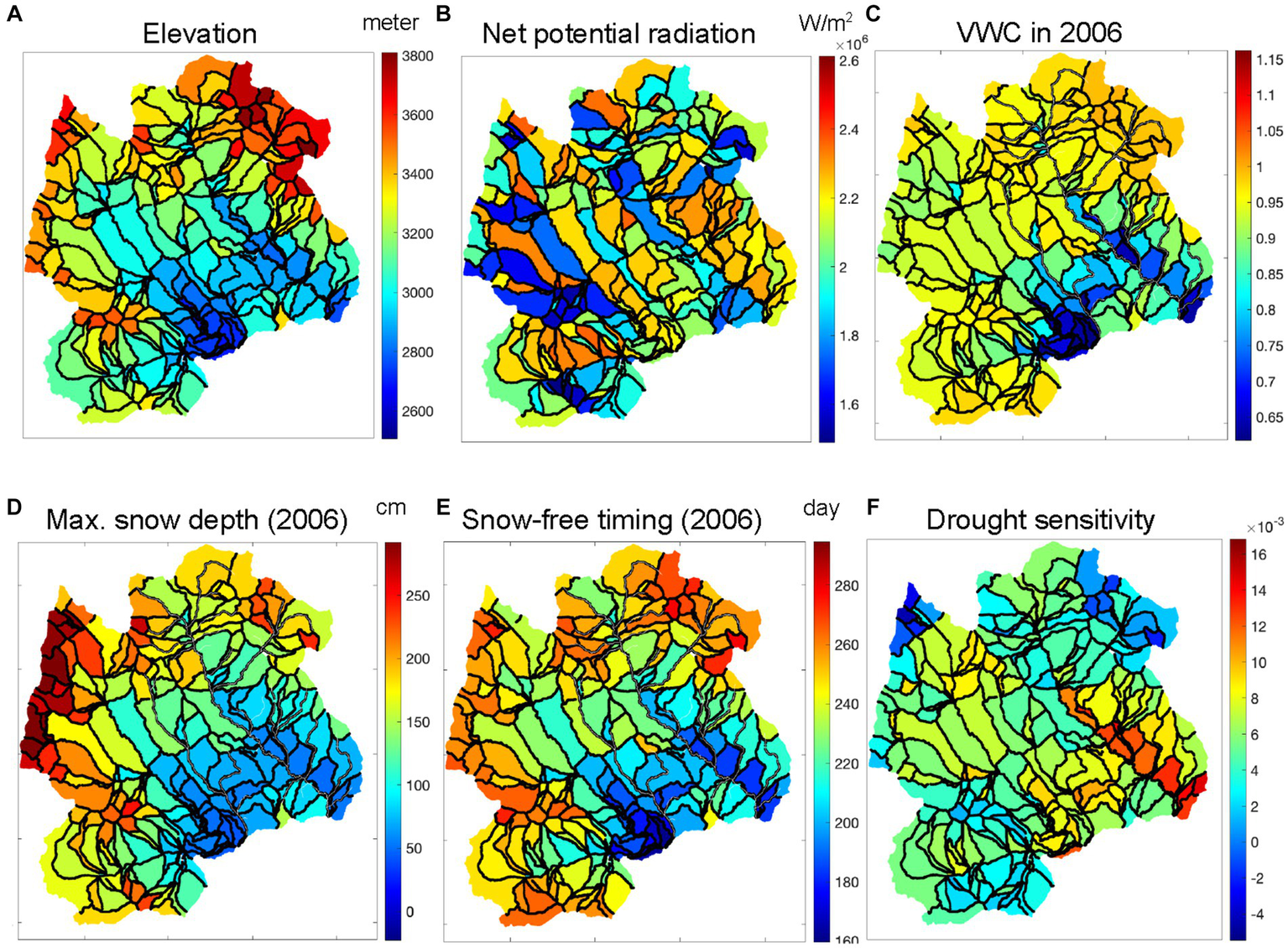
Spatial distributions of hillslope features: (A) elevation, (B) annual net potential radiation, (C) growing-season-average soil moisture in 2006, (D) max snow depth in 2006, (E) snow-free timing in 2006, and (F) drought sensitivity. The black lines are the hillslope boundaries.
The correlation among the hillslope features was discussed in Wainwright et al. (2020) and Maina et al. (2021), although here we added additional features such as soil moisture and snow-free timing (Figures 3, 4). In addition to the average year 2006, we added the difference between 1995 (extreme wet water year) and 2012 (extreme dry water year) to represent the year-to-year variability. The average growing-season soil moisture is correlated with the elevation and snow-free timing except for 1995. The correlations are consistent with the observations from the maps (Figure 2), such that soil moisture increases with elevation and snow-free timing. The correlation coefficient is higher in the dry year (2012), while the lowest is in the wet year (1995). The dependency is non-linear, such that soil moisture does not increase above the threshold elevation (3,000–3,200 m) and snow-free timing (200–220 days). Soil moisture in 2006 was non-linearly correlated with elevation, with soil moisture increasing up to 3,300 m but no further. The drought sensitivity (Figure 4) is most closely correlated with the difference in soil moisture between the wet year (1995) and dry year (2012). The correlation is positive across the space, meaning that the larger soil-moisture variability hillslopes have higher sensitivity. Although other metrics are correlated with drought sensitivity, the correlations are lower.
Figure 3
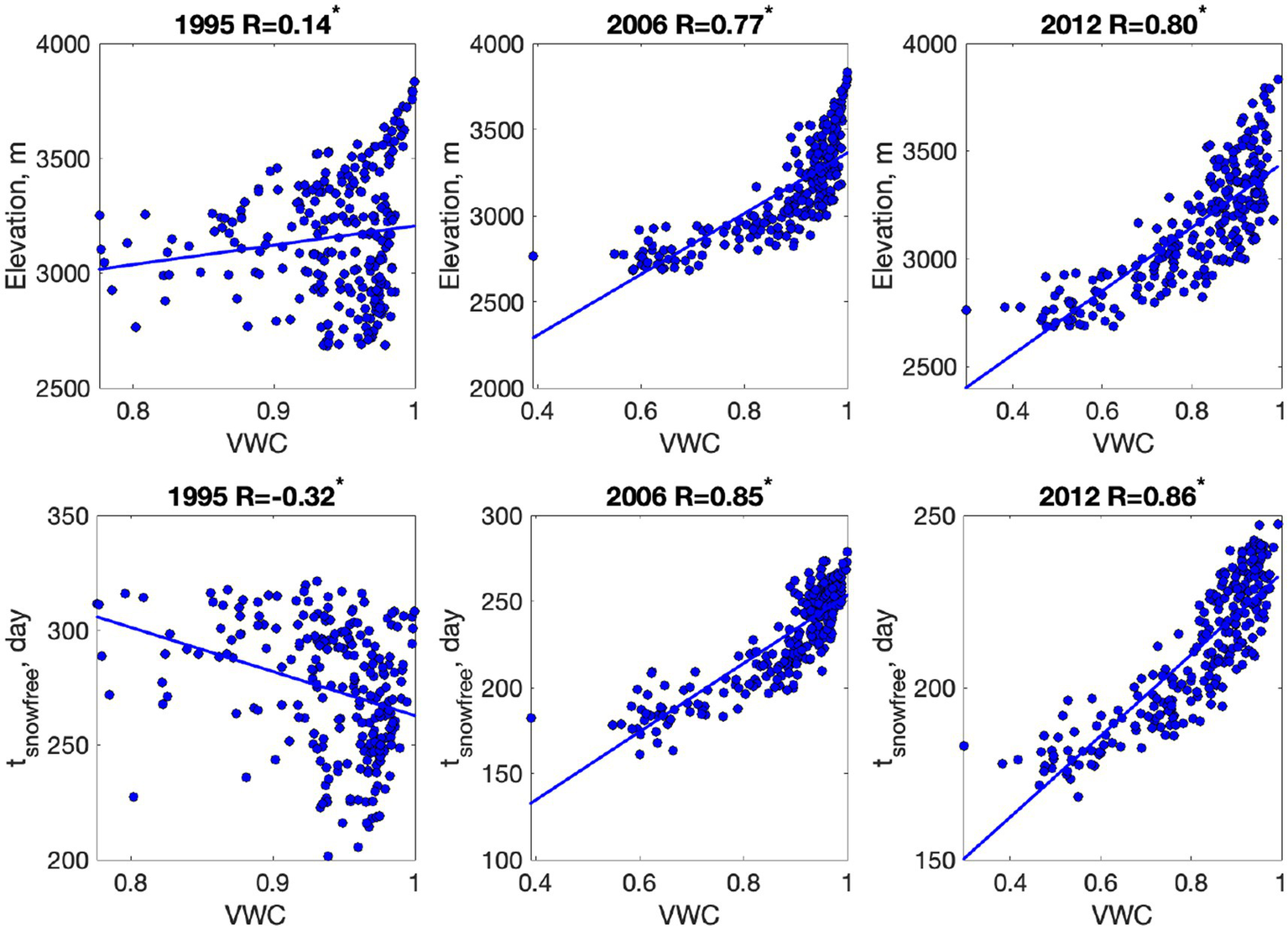
Correlation between the average growing-season soil moisture (volumetric water content, VWC) with elevation (the upper row) and snow-free timing (the lower row) in three distinct years. The correlation coefficient (R) is added above each plot, while * represents that the correlation is statistically significant, with a value of p of 0.01.
Figure 4
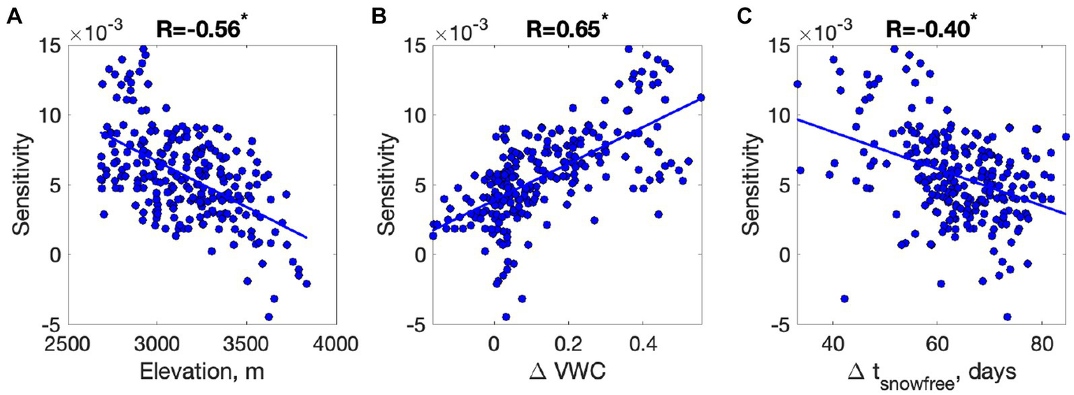
Foresummer drought sensitivity as a function of (A) elevation and the difference between wet (1995) and dry (2012) years in (B) soil moisture (ΔVWC) and (C) snow-free timing (Δtsnowfree). The correlation coefficient (R) is added above each plot, while * represents that the correlation is statistically significant with a value of p of 0.01.
The RF regression for the foresummer drought sensitivity shows predictive performance with a coefficient of determination (R-square) of 0.65 (value of p of 0.01). The importance ranking (see Table 1) is measured by the percentage of the mean-squared error difference when each feature is dropped. Radiation, elevation, and soil moisture differences are among the strongest predictors of foresummer drought sensitivity. Then, snow-free timing in the average year (2006) and its difference between the extreme years follow in the ranking. The snow depth-related features are relatively weak predictors.
Table 1
| %MSE | |
|---|---|
| Radiation | 19.2 |
| Diff. VWC | 19.0 |
| Elevation | 16.8 |
| Snow-free timing in 2006 | 13.9 |
| Diff. snow-free timing | 13.6 |
| Diff. max-snow timing | 12.4 |
| Av. VWC in 2006 | 11.2 |
| Max-snow timing in 2006 | 9.8 |
| Max snow depth in 2006 | 8.4 |
| Diff. max snow depth | 7.4 |
Parameter importance ranking from the random forest analysis; the features influencing the spatial heterogeneity of foresummer drought sensitivity.
The importance measure is the percent increase in the mean-squared error when each feature is removed.
4.2 Step 2: clustering analysis results
The GMM clustering identified the optimal number of clusters as five. The relationship among the predictors is shown in the PCA bi-plot (Figure 5A). The first two components explain 80% of the variability. The first PC has high loadings from the soil moisture difference between 2012 and 1995, as well as elevation. The second component has the net potential radiation and maximum snow timing. Drought sensitivity is between the first and second components, representing the positive correlations, particularly with the soil moisture difference and radiation.
Figure 5
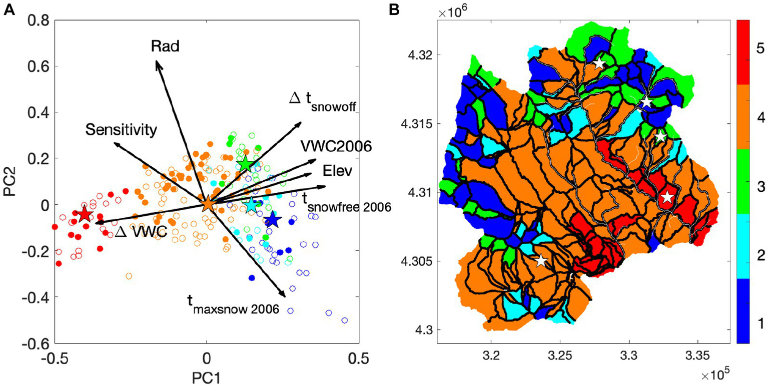
(A) PCA biplot with the first and second components (PC1 and PC2), and (B) the zonation map with five zones. In panel (A), the arrows represent the loading of each feature, while the circles represent the score of each data point. The circles represent all the hillslopes, while the filled circles are the ones with trail/road access. In (B), the five different colors represent different zones. In panels (A,B), the stars represent the most representative hillslopes in each zone with road/trail access.
The identified zones capture the co-varied heterogeneity along these two PCs and these features. Zone 5 represents the region with the lowest elevation and the largest soil moisture variability (ΔVWC). Zone 4 is around the center of the PC1-PC2 space, and the middle region of these features. Zones 1–3 are in the higher elevation region with lower soil moisture variability; however, they are differentiated by the radiation and maximum snow-timing, which are both related to the sensitivity. Zone 1 represents north-facing hillslopes with late maximum snow timing. The hillslopes with road/trail access cover the range of these features, although the high-elevation hillslopes are not accessible. The stars indicate the representative and accessible hillslopes in the five zones.
In Figure 5B, the zones are distributed according to the features relevant to drought sensitivity. Zone 1 represents the least sensitive region with high elevation, late maximum snow timing, and north-facing hillslopes. Zone 2 and 3 are hillslopes with low sensitivity, although Zone 2 is generally north-facing and has higher net potential radiation than Zone 3. Zone 4 is in the intermediate zone, while Zone 5 is the highest sensitivity zone. The area coverage of each zone in the domain is 17.0% for Zone 1, 8.0% for Zone 2, 11.9% for Zone 3, 54.5% for Zone 4, and 8.6% for Zone 5. Although Zone 4 has the largest spatial coverage, its features are concentrated in Figure 5A, suggesting that the hillslopes in Zone 4 are similar to each other with respect to these features. Within each zone, the most representative hillslope with site access is selected. The selected hillslopes for Zones 1–3 are all in the northeastern region, which is due to the fact that Zones 1–3 represent higher elevation regions and trail access is limited in the northwestern regions.
5 Discussion
In this study, we extended the approach by Wainwright et al. (2022a) and Maina et al. (2021) to include both key observed data from remote sensing on plant productivity (i.e., foresummer drought sensitivity) and model-computed hydrological variables (soil moisture and snow depth). We used the same clustering approach to compress multidimensional data and identify zones that capture co-varied properties. This approach enables us to explore the effect of water limitation on plant productivity as well as snow-soil–plant interactions over space and time. In addition, we added an extra step to identify the most representative and accessible hillslopes for future sampling to enable a model-experimental (ModEx) design [Department of Energy (DOE), 2023].
The results show that soil moisture variability is the best predictor of foresummer drought sensitivity. This is consistent with the current understanding of the water limitation on plant productivity in this region (Sloat et al., 2015). At the same time, this fact also adds more confidence to the model results. Although soil moisture and snow thickness are known to be highly heterogeneously impacted by microtopography (Falco et al., 2019; Devadoss et al., 2020), the model results capture the general trend and variability of soil moisture across the watershed. However, the floodplain area in the Slate watershed shows a surprising discrepancy, in the sense that while the soil moisture and elevation are both low, the sensitivity is not quite as high as in other regions with similar soil moisture values. Since its upstream hillslopes tend to have significant snow accumulation at high elevations, it would be possible that this low-elevation region benefited more from stream and/or subsurface water from the upper watersheds. This discrepancy suggests the need for further investigation into this region and potentially some model refinements.
The predictive performance of foresummer drought sensitivity is higher with hydrological variables (e.g., ΔVWC) compared to the static explanatory variables (such as elevation, geology, and other parameters used in Wainwright et al., 2020). This is potentially a result of the non-linearity among soil moisture, snowmelt timing, and elevation. The model-derived soil moisture physically aggregates multiple parameters and effects, such as elevation, aspects, and hydrological gradient, into a single variable that is more effective in describing the water limitation on plant productivity. Although the obtained zonation map is quite similar to the one based only on the remote sensing data in Wainwright et al. (2022a,b), there are some differences. This zonation map based on both remote sensing and modeling results has more zones at higher elevations (Zones 1–3). This is attributed to the non-linearity, such that the snow-free timing is more heterogeneous than other variables influenced by radiation at similar elevations. This also suggests that, while currently the elevation and elevation-based life zones (such as montane, subalpine, and alpine) are often used to represent the distinct ecosystem zones, model-based metrics can be used to further refine these distinct zones.
Additionally, the combination of satellite observation data and modeling results may provide alternative hypotheses for snow-soil–plant interactions. The snow-soil–plant interactions under climate change have been extensively studied in the recent decade (e.g., Schmidt and Lipson, 2004; Brooks et al., 2011; Sanders-DeMott et al., 2018). Different mechanisms and processes are considered, such as increased soil warming (Melillo et al., 2011), microbial or biogeochemical impacts (Schmidt and Lipson, 2004; Brooks et al., 2011), and the decrease in snowpack reducing insulation and increasing freezing-induced root damage (Sanders-DeMott et al., 2018). In our study domain, as mentioned above, plant productivity is considered to be limited by water availability, such that early snowmelt leads to early soil drying and creates drought conditions before the summer monsoon (Sloat et al., 2015; Dafflon et al., 2023). Although this study confirms this hypothesis, it also suggests a non-linear interaction across space and time and the presence of threshold values.
In our results, soil moisture is correlated with snow-free timing, but the relationship is non-linear. In the high-elevation north-facing region, as well as in the big snow year, the soil moisture does not depend on snow-free timing because soil moisture becomes saturated due to the deep snowpack, limited soil storage, and the lateral transfer of water from high alpine regions to upper subalpine zones (Carroll et al., 2019). In dry years and low-elevation regions, the correlation is more significant, suggesting these conditions and/or locations are soil moisture-limited. Based on these results, we may hypothesize that these regions, which are currently resilient to year-to-year climate variability, may become more sensitive to the variability in the future as the temperature increases and snow depth decreases at higher elevations. Since such non-linearity is difficult to detect through sparse measurements, spatially continuous modeling results are likely the most effective way to identify non-linearity and threshold processes.
We would note that, in this study, we did not consider the antecedent conditions from the previous year. We assumed that it could be limited in this system because, due to snow and thin soils in the montane-alpine region, the soil becomes fully saturated after snowmelt every year. Such a soil storage limitation has been reported in other regions (Hahm et al., 2019), and its impact on plant dynamics would be interesting to investigate in subsequent studies.
Our approach also identifies the different zones—i.e., the hillslope groups—that potentially have divergent snow-soil–plant interactions. In addition to the low- and high-sensitivity regions, clustering identified the intermediate- to higher-elevation regions where the topographic aspects are considered to play key controls. As global warming continues, snow-free timing is expected to decrease, but may or may not do so below the threshold in these regions since the topography is not likely to change in the same time frame as climate. In this future scenario, the steep hillslopes and the large variability of aspects and potential radiations would increase the spatial heterogeneity of drought sensitivities.
This type of monitoring design methodology is expected to be increasingly important as sensor and telecommunication technologies improve and a wide variety of fixed/permanent sensors are available (e.g., Hubbard et al., 2018). The U.S. Geological Survey’s Next Generation Water Observing System, for example, plans to have distributed sensors and observational sites for soil moisture, snow-water-equivalent, and others (US Geological Survey, 2023). In addition, sporadic ground-based surveys such as snow course measurements are still important to cover a larger space between fixed sensors and to create site-specific relationships with remote sensing data (Dressler et al., 2006). In particular, our approach is promising to guide the optimal deployment of wireless sensor networks (e.g., Oroza et al., 2016; Wielandt et al., 2023), in which the value of sensing various properties of interest might need to be balanced by the site accessibility, sensor resolution and accuracy, power requirement, wireless connectivity, total data cost, and complementarity to remote sensing products and other datasets.
Finally, this study shows the power of combining remote sensing data and modeling results to locate key observation locations and generate hypotheses that can be applied to other processes. Although plant productivity and trait data are increasingly available over time and space, subsurface properties are largely considered to be a “black box” (Sevanto et al., 2020). The modeling results are particularly powerful in this regard, providing subsurface state variables such as soil moisture. In addition, our method can determine the most representative hillslope in each zone that has road/trail access, which facilitates the selection of experiment/monitoring sites. The consideration of road/trail access could be easily extended to incorporate additional objectives in the site selection process. Now that ML approaches are widely available and more people are trained to use ML for extracting critical patterns in spatial data layers, model-guided monitoring design and hypothesis generation can be more readily employed in critical zone and watershed sciences.
Statements
Data availability statement
Publicly available datasets were analyzed in this study. This data can be found at: the datasets are located on the U.S. Department of Energy repository ESS-DIVE: the simulation data link (https://data.ess-dive.lbl.gov/datasets/doi:10.15485/1889747) and the remote sensing data link (https://doi.org/10.15485/1841262).
Author contributions
HW performed statistical analyses and wrote the main text. NF processed remote sensing data layers and contributed to the manuscript. ES-W and RC provided model results and contributed to the manuscript. BD, IB, and YW provided perspectives on monitoring and sensor network and contributed to the manuscript. All authors contributed to the article and approved the submitted version.
Funding
This material is based upon work supported as part of the Watershed Function Scientific Focus Area funded by the U.S. Department of Energy, Office of Science, Office of Biological and Environmental Research under Award Number DE-AC02-05CH11231.
Acknowledgments
The datasets are available in the study by Wainwright et al. (2022b) for the remote sensing data layers and the study by Carroll (2022) for the model data layers. We thank Dan Hawkes for editing, the two reviewers, and the editor, Erin Seybold.
Conflict of interest
The authors declare that the research was conducted in the absence of any commercial or financial relationships that could be construed as a potential conflict of interest.
Publisher’s note
All claims expressed in this article are solely those of the authors and do not necessarily represent those of their affiliated organizations, or those of the publisher, the editors and the reviewers. Any product that may be evaluated in this article, or claim that may be made by its manufacturer, is not guaranteed or endorsed by the publisher.
Footnotes
References
1
Bierkens M. F. Bell V. A. Burek P. Chaney N. Condon L. E. David C. H. et al . (2015). Hyper-resolution global hydrological modelling: what is next? “Everywhere and locally relevant”. Hydrol. Process.29, 310–320. doi: 10.1002/hyp.10391
2
Breiman L. (2001). Random forests. Mach. Learn.45, 5–32.
3
Brooks P. D. Grogan P. Templer P. H. Groffman P. Öquist M. G. Schimel J. (2011). Carbon and nitrogen cycling in snow-covered environments. Geogr. Compass5, 682–699. doi: 10.1111/j.1749-8198.2011.00420.x
4
Carroll R. (2022): Model files for estimating snow dynamics and stable water isotopes across the East River, CO. watershed function SFA, ESS-DIVE repository. Dataset. Available at: https://data.ess-dive.lbl.gov/datasets/doi:10.15485/1889747 (Accessed 16 August 2023)
5
Carroll R. W. Deems J. Maxwell R. Sprenger M. Brown W. Newman A. et al . (2022a). Variability in observed stable water isotopes in snowpack across a mountainous watershed in Colorado. Hydrol. Process.36:e14653. doi: 10.1002/hyp.14653
6
Carroll R. W. Deems J. Sprenger M. Maxwell R. Brown W. Newman A. et al . (2022b). Modeling snow dynamics and stable water isotopes across mountain landscapes. Geophys. Res. Lett.49:e2022GL098780. doi: 10.1029/2022GL098780
7
Carroll R. W. H. Deems J. S. Niswonger R. Schumer R. Williams K. H. (2019). The importance of interflow to groundwater recharge in a snowmelt-dominated headwaterbasin. Geophys. Res. Lett.46, 5899–5908. doi: 10.1029/2019GL082447
8
Chadwick K. D. Brodrick P. G. Grant K. Goulden T. Henderson A. Falco N. et al . (2020). Integrating airborne remote sensing and field campaigns for ecology and earth system science. Methods Ecol. Evol.11, 1492–1508. doi: 10.1111/2041-210X.13463
9
Condon L. E. Maxwell R. M. (2015). Evaluating the relationship between topography and groundwater using outputs from a continental-scale integrated hydrology model. Water Resour. Res.51, 6602–6621. doi: 10.1002/2014WR016774
10
Dafflon B. Léger E. Falco N. Wainwright H. M. Peterson J. Chen J. et al . (2023). Advanced monitoring of soil-vegetation co-dynamics reveals the successive controls of snowmelt on soil moisture and on plant seasonal dynamics in a mountainous watershed. Front. Earth Sci.11:976227. doi: 10.3389/feart.2023.976227
11
Department of Energy (DOE) (2023) ModEx Approach. Available at: https://ess.science.energy.gov/modex/ (Accessed 16 August 2023).
12
Devadoss J. Falco N. Dafflon B. Wu Y. Franklin M. Hermes A. et al . (2020). Remote sensing-informed zonation for understanding snow, plant and soil moisture dynamics within a mountain ecosystem. Remote Sens. (Basel)12:2733. doi: 10.3390/rs12172733
13
Dong C. MacDonald G. M. Willis K. Gillespie T. W. Okin G. S. Williams A. P. (2019). Vegetation responses to 2012–2016 drought in northern and Southern California. Geophys. Res. Lett.46, 3810–3821. doi: 10.1029/2019GL082137
14
Dressler K. A. Fassnacht S. R. Bales R. C. (2006). A comparison of snow telemetry and snow course measurements in the Colorado River basin. J. Hydrometeorol.7, 705–712. doi: 10.1175/JHM506.1
15
Enguehard L. Falco N. Schmutz M. Newcomer M. E. Ladau J. Brown J. B. et al . (2022). Machine-learning functional zonation approach for characterizing terrestrial–aquatic interfaces: application to Lake Erie. Remote Sens. (Basel)14:3285. doi: 10.3390/rs14143285
16
Falco N. Balde A. Breckheimer I. Brodie E. Brodrick P. Chadwick K. D. et al . (2020). Plant species distribution within the upper Colorado River basin estimated by using hyperspectral and LiDAR airborne data. Watershed function SFA.
17
Falco N. Wainwright H. Dafflon B. Léger E. Peterson J. Stelzer H. et al . (2019). Remote sensing and geophysical characterization of a floodplain-hillslope system in the East River watershed, Colorado. Watershed Functionality Scientific Focus Area.
18
Hahm W. J. Dralle D. N. Rempe D. M. Bryk A. B. Thompson S. E. Dawson T. E. et al . (2019). Low subsurface water storage capacity relative to annual rainfall decouples Mediterranean plant productivity and water use from rainfall variability. Geophys. Res. Lett.46, 6544–6553. doi: 10.1029/2019GL083294
19
Hastie T. Tibshirani R. Friedman J. H. Friedman J. H. (2009). The elements of statistical learning: data mining, inference, and prediction. New York. 2, 1–758.
20
Hermes A. L. Wainwright H. M. Wigmore O. H. Falco N. Molotch N. Hinckley E. L. S. (2020). From patch to catchment: a statistical framework to identify and map soil moisture patterns across complex alpine terrain. Front Water2:48. doi: 10.3389/frwa.2020.578602
21
Hubbard S. S. Williams K. H. Agarwal D. Banfield J. Beller H. Bouskill N. et al . (2018). The East River, Colorado, watershed: a mountainous community testbed for improving predictive understanding of multiscale hydrological–biogeochemical dynamics. Vadose Zone J.17, 1–25. doi: 10.2136/vzj2018.03.0061
22
Kerkez B. Glaser S. D. Bales R. C. Meadows M. W. (2012). Design and performance of a wireless sensor network for catchment-scale snow and soil moisture measurements. Water Resour. Res.48:214. doi: 10.1029/2011WR011214
23
Knowles J. F. Lestak L. R. Molotch N. P. (2017). On the use of a snow aridity index to predict remotely sensed forest productivity in the presence of bark beetle disturbance. Water Resour. Res.53, 4891–4906. doi: 10.1002/2016WR019887
24
Knowles J. F. Molotch N. P. Trujillo E. Litvak M. E. (2018). Snowmelt-driven trade-offs between early and late season productivity negatively impact Forest carbon uptake during drought. Geophys. Res. Lett.45, 3087–3096. doi: 10.1002/2017GL076504
25
Landfire . (2015). “Existing vegetation type and cover layers,” in U.S. Department of the Interior, Geological Survey. Available at: http://landfire.cr.usgs.gov/viewer/
26
Li L. (2019). Watershed reactive transport. Rev. Mineral. Geochem.85, 381–418. doi: 10.2138/rmg.2018.85.13
27
Li L. Maher K. Navarre-Sitchler A. Druhan J. Meile C. Lawrence C. et al . (2017). Expanding the role of reactive transport models in critical zone processes. Earth Sci. Rev.165, 280–301. doi: 10.1016/j.earscirev.2016.09.001
28
Maavara T. Siirila-Woodburn E. R. Maina F. Maxwell R. M. Sample J. E. Chadwick K. D. et al . (2021). Modeling geogenic and atmospheric nitrogen through the East River watershed, Colorado Rocky Mountains. PloS One16:e0247907. doi: 10.1371/journal.pone.0247907
29
Madritch M. D. Kingdon C. C. Singh A. Mock K. E. Lindroth R. L. Townsend P. A. (2014). Imaging spectroscopy links aspen genotype with below-ground processes at landscape scales. Philosoph Trans R Soc B Biol Sci369:20130194. doi: 10.1098/rstb.2013.0194
30
Maina F. Z. Wainwright H. M. Dennedy-Frank P. J. Siirila-Woodburn E. R. (2021). On the similarity of hillslope hydrologic function: a process-based approach. Hydrol. Earth Syst. Sci. Discuss.26, 3805–3823. doi: 10.5194/hess-2021-520
31
McLachlan G. Peel D. (2004) Finite Mixture Models. Wiley.
32
Melillo J. M. Butler S. Johnson J. Mohan J. Steudler P. Lux H. et al . (2011). Soil warming, carbon–nitrogen interactions, and forest carbon budgets. Proc. Natl. Acad. Sci.108, 9508–9512. doi: 10.1073/pnas.1018189108
33
Mirus B. B. Ebel B. A. Mohr C. H. Zegre N. (2017). Disturbance hydrology: preparing for an increasingly disturbed future. Water Resour. Res.53, 10007–10016. doi: 10.1002/2017WR021084
34
Newcomer M. E. Underwood J. Murphy S. F. Ulrich C. Schram T. Maples S. R. et al . (2023). Prolonged drought in a northern California coastal region suppresses wildfire impacts on hydrology. Water Resour. Res.:e2022WR034206. doi: 10.1029/2022WR034206
35
Oroza C. A. Zheng Z. Glaser S. D. Tuia D. Bales R. C. (2016). Optimizing embedded sensor network design for catchment-scale snow-depth estimation using LiDAR and machine learning. Water Resour. Res.52, 8174–8189. doi: 10.1002/2016WR018896
36
Painter T. H. Berisford D. F. Boardman J. W. Bormann K. J. Deems J. S. Gehrke F. et al . (2016). The airborne snow observatory: fusion of scanning lidar, imaging spectrometer, and physically-based modeling for mapping snow water equivalent and snow albedo. Remote Sens. Environ.184, 139–152. doi: 10.1016/j.rse.2016.06.018
37
Parsekian A. D. Singha K. Minsley B. J. Holbrook W. S. Slater L. (2015). Multiscale geophysical imaging of the critical zone. Rev. Geophys.53, 1–26. doi: 10.1002/2014RG000465
38
Patton N. R. Lohse K. A. Godsey S. E. Crosby B. T. Seyfried M. S. (2018). Predicting soil thickness on soil mantled hillslopes. Nat. Commun.9:3329. doi: 10.1038/s41467-018-05743-y
39
Pedregosa F. Varoquaux G. Gramfort A. Michel V. Thirion B. Grisel O. et al . (2011). Scikit-learn: Machine learning in Python. J. Mach. Learn. Res.12, 2825–2830.
40
Pelletier J. D. Barron-Gafford G. A. Gutiérrez-Jurado H. Hinckley E. L. S. Istanbulluoglu E. McGuire L. A. et al . (2018). Which way do you lean? Using slope aspect variations to understand critical zone processes and feedbacks. Earth Surf. Process. Landf.43, 1133–1154. doi: 10.1002/esp.4306
41
Sanders-DeMott R. McNellis R. Jabouri M. Templer P. H. (2018). Snow depth, soil temperature and plant–herbivore interactions mediate plant response to climate change. J. Ecol.106, 1508–1519. doi: 10.1111/1365-2745.12912
42
Schmidt S. K. Lipson D. A. (2004). Microbial growth under the snow: implications for nutrient and allelochemical availability in temperate soils. Plant and Soil259, 1–7. doi: 10.1023/B:PLSO.0000020933.32473.7e
43
Schwanghart W. Dirk S. (2014). “TopoToolbox 2–MATLAB-based software for topographic analysis and modeling in Earth surface sciences.” Earth Surface Dynamics2, 1–7.
44
Schwanghart W. Kuhn N. J. (2010). TopoToolbox: A set of Matlab functions for topographic analysis. Environ. Model. Softw.25, 770–781.
45
Sevanto S. Grossiord C. Klein T. Reed S. (2020). Plant-soil interactions under changing climate. Front. Plant Sci.11:621235. doi: 10.3389/fpls.2020.621235
46
Siirila-Woodburn E. R. Rhoades A. M. Hatchett B. J. Huning L. S. Szinai J. Tague C. et al . (2021). A low-to-no snow future and its impacts on water resources in the western United States. Nat Rev Earth Environ2, 800–819. doi: 10.1038/s43017-021-00219-y
47
Sivapalan M . (2006). “Pattern, process and function: elements of a unified theory of hydrology at the catchment scale,” inEncyclopedia of hydrological sciences. eds. AndersonM. G.McDonnellJ. J..
48
Sloat L. Henderson A. Lamanna C. Enquist B. (2015). The effect of the Foresummer drought on carbon exchange in subalpine Meadows. Ecosystems18, 533–545. doi: 10.1007/s10021-015-9845-1
49
Strachan S. Kelsey E. P. Brown R. F. Dascalu S. Harris F. Kent G. et al . (2016). Filling the data gaps in mountain climate observatories through advanced technology, refined instrument siting, and a focus on gradients. Mt. Res. Dev.36, 518–527. doi: 10.1659/MRD-JOURNAL-D-16-00028.1
50
Uhlemann S. Dafflon B. Wainwright H. M. Williams K. H. Minsley B. Zamudio K. et al . (2022). Surface parameters and bedrock properties covary across a mountainous watershed: insights from machine learning and geophysics. Sci. Adv.8:eabj2479. doi: 10.1126/sciadv.abj2479
51
US Geological Survey , (2023), Next generation water observing system: upper Colorado River basin, Available at: https://www.usgs.gov/mission-areas/water-resources/science/next-generation-water-observing-system-upper-colorado-river#science (Accessed 15 August 2023).
52
Wagener T. Sivapalan M. Troch P. Woods R. (2007). Catchment classification and hydrologic similarity. Geogr. Compass1, 901–931. doi: 10.1111/j.1749-8198.2007.00039.x
53
Wainwright H. M. Dafflon B. Smith L. J. Hahn M. S. Curtis J. B. Wu Y. et al . (2015). Identifying multiscale zonation and assessing the relative importance of polygon geomorphology on carbon fluxes in an Arctic tundra ecosystem. J. Geophys. Res. Biogeo.120, 788–808. doi: 10.1002/2014JG002799
54
Wainwright H. M. Steefel C. Trutner S. D. Henderson A. N. Nikolopoulos E. I. Wilmer C. F. et al . (2020). Satellite-derived foresummer drought sensitivity of plant productivity in Rocky Mountain headwater catchments: spatial heterogeneity and geological-geomorphological control. Environ. Res. Lett.15:084018. doi: 10.1088/1748-9326/ab8fd0
55
Wainwright H. M. Uhlemann S. Franklin M. Falco N. Bouskill N. J. Newcomer M. E. et al . (2022a). Watershed zonation through hillslope clustering for tractably quantifying above-and below-ground watershed heterogeneity and functions. Hydrol. Earth Syst. Sci.26, 429–444. doi: 10.5194/hess-26-429-2022
56
Wainwright H. M. Uhlemann S. Franklin M. Falco N. Bouskill N. Newcomer M. et al . (2022b): “Watershed zonation through hillslope clustering for tractably quantifying above- and belowground watershed heterogeneity and functions”. Watershed Function SFA, ESS-DIVE repository. Dataset. Available at: https://data.ess-dive.lbl.gov/datasets/doi:10.15485/1841262 (Accessed 16 August 2023)
57
Wielandt S. Uhlemann S. Fiolleau S. Dafflon B. (2023). TDD LoRa and Delta encoding in low-power networks of environmental sensor arrays for temperature and deformation monitoring. J Signal Process Syst95, 831–843. doi: 10.1007/s11265-023-01834-2
58
Xu Z. Molins S. Özgen-Xian I. Dwivedi D. Svyatsky D. Moulton J. D. et al . (2022). Understanding the hydrogeochemical response of a mountainous watershed using integrated surface-subsurface flow and reactive transport modeling. Water Resour. Res.58:e2022WR032075. doi: 10.1029/2022WR032075
59
Yan Q. Haruko W. Baptiste D. Sebastian U. Carl S. Nicola F. et al . (2020) Hybrid data-model-based mapping of soil thickness in a mountainous watershed., submitted to earth surface dynamics.
60
Zhang D. Heery B. O’Neil M. Little S. O’Connor N. E. Regan F. (2019). A low-cost smart sensor network for catchment monitoring. Sensors19:2278. doi: 10.3390/s19102278
Summary
Keywords
hillslope, watershed, machine learning, clustering, Gaussian mixture model, random forest, zonation
Citation
Wainwright HM, Dafflon B, Siirila-Woodburn ER, Falco N, Wu Y, Breckheimer I and Carroll RWH (2024) Model and remote-sensing-guided experimental design and hypothesis generation for monitoring snow-soil–plant interactions. Front. Water 5:1220146. doi: 10.3389/frwa.2023.1220146
Received
10 May 2023
Accepted
16 November 2023
Published
08 January 2024
Volume
5 - 2023
Edited by
Erin Seybold, University of Kansas, United States
Reviewed by
Michael Tso, UK Centre for Ecology and Hydrology (UKCEH), United Kingdom; Xiang Zhang, China University of Geosciences Wuhan, China
Updates
Copyright
© 2024 Wainwright, Dafflon, Siirila-Woodburn, Falco, Wu, Breckheimer and Carroll.
This is an open-access article distributed under the terms of the Creative Commons Attribution License (CC BY). The use, distribution or reproduction in other forums is permitted, provided the original author(s) and the copyright owner(s) are credited and that the original publication in this journal is cited, in accordance with accepted academic practice. No use, distribution or reproduction is permitted which does not comply with these terms.
*Correspondence: Haruko M. Wainwright, hmwainw@mit.edu
Disclaimer
All claims expressed in this article are solely those of the authors and do not necessarily represent those of their affiliated organizations, or those of the publisher, the editors and the reviewers. Any product that may be evaluated in this article or claim that may be made by its manufacturer is not guaranteed or endorsed by the publisher.