River reach-level machine learning estimation of nutrient concentrations in Great Britain

Nitrogen (N) and phosphorus (P) are essential nutrients necessary for plant growth and support life in aquatic ecosystems. However, excessive N and P can lead to algal blooms that deplete oxygen and lead to fish death and the release of toxins that are harmful to humans. Estimates of N and P levels in rivers are typically calculated at station or grid (>1 km) scale; therefore, it is difficult to visualise the evolution of water quality as water travels downstream. Using a high-resolution reach-scale river network and associating each reach with land cover fractions and catchment descriptors, we trained random forest models on aggregated data (2010–2020) from the Environmental Agency Open Water Quality Data Archive for 2,343 stations to predict long-term nitrate and orthophosphate concentrations at each river reach in Great Britain (GB). We separated the model training and predictions for different seasons to investigate the potential difference in feature importance. Our model predicted concentrations with an average testing coefficient of determination (R²) of 0.71 for nitrate and 0.58 for orthophosphate using 5-fold cross-validation. Our model showed slightly better performance for higher Strahler stream orders, highlighting the challenges of making predictions in small streams. Our results revealed that arable and horticultural land use is the strongest and most reliable predictor for nitrate, while floodplain extents and standard percentage runoff are stronger predictors for orthophosphate. Nationally, higher orthophosphate concentrations were observed in urbanised areas. This study shows how combining a river network model with machine learning can easily provide a river network understanding of the spatial distribution of water quality levels.

Highlights

- A method to map point water quality observations to river reaches is developed.

- Catchment descriptors and land covers are mapped to reaches and used as input features.

- Random forest models perform well for nitrate and orthophosphate over Great Britain.

1. Introduction

Anthropogenic demands for food, energy, and raw materials have reshaped the abundance and recycling of nitrogen (N) and phosphorus (P). Excess N and P input to the landscape can contaminate drinking water supplies and accelerate eutrophication, though they are important nutrients for plant and algal growth. To meet the UN Sustainable Development Goals, it has been argued that we must eliminate nutrient overuse and still allow a 30% increase in the production of major cereals (Mueller et al., 2012).

Reliable prediction and modelling underpin water quality management practises. However, the abundances of N and P in rivers are controlled by multiple factors, and often, the physical process is not easily observed. Therefore, it is challenging to model N and P distribution for large areas or at high frequencies using physically based process models. The mapping of nutrients in rivers has traditionally been performed using statistical models. Because data are sparse, many early efforts focussed on statistical modelling in small catchments using methods such as general linear models and non-linear estimation models (Howden and Burt, 2009) or generalised additive models (Morton and Henderson, 2008; Yang and Moyer, 2020). These aimed to provide a robust regression for the estimation of non-linear trends in water quality in the presence of potentially correlated errors.

A very different type of modelling framework is the Source Apportionment Geographical Information System (SAGIS), which uses readily available national datasets to estimate concentrations of nutrients, among other chemicals, from multiple sector sources (Comber et al., 2013). Concentrations and loads are modelled using the Environment Agency's catchment river model, SIMCAT, at the locations of model features or every 1 km along each river, taking into account all upstream sources and user defined river losses. Similarly, the GREEN model is a simple three-parameter statistical model for source apportionment of riverine nutrient loads and has been applied widely across the European Union (Grizzetti et al., 2005). Finally, process-based models are also used to simulate the chemical and biological status of river networks (Evans et al., 2006). For example, INCA is a semi-distributed catchment model that is widely used in the UK and globally and can account for diffuse and point sources of pollution, land use change, and climate change (Whitehaed et al., 1998). This is done by accounting for all input sources and driving data and accounting for the process pathways in different compartments (e.g., soil horizon, groundwater zone, in-stream water column, streambed, and sediments).

Recently, machine learning methods have been increasingly applied to water quality predictions (see review by Najah Ahmed et al., 2019). While a small number of studies focus on classifying waters into discrete classes (O'Sullivan et al., 2022), most research seeks to predict quantitative values using regression. An important distinction within water quality machine learning applications is that while some focus on high-frequency predictions (i.e., daily or sub-daily), others focus on long-term or seasonal predictions. The former focuses on capturing the rapid dynamics of the system in response to changes in input variables and could be used for near real-time monitoring and early warning systems, while the latter is often applied to a large area and seeks to improve understanding of the key controls of overall water quality trends. For the first group, examples include Xu et al. (2021), who compared eight machine learning regressions to predict total nitrogen (TN) in the Lianjiang River basin, Guangdong, China; Granata et al. (2017), who compared support vector machines and regression trees to predict wastewater quality from surrogate variables and training data from the US National Stormwater Quality Database; and Ahmed et al. (2019), who compared the use of 15 supervised machine learning methods for water quality index predictions. Examples of the second group include the use of random forest modelling to explore the relationships between stream N and watershed features, climate, and N input rates at nearly 5,000 US watersheds (Lin J. et al., 2021). In another study (Frei et al., 2021), the importance of land use and land cover for lake vs. stream on water quality were compared using four machine learning methods. Bhattarai et al. (2021) used ML algorithms to predict nitrate and total phosphorus for five watersheds of different types draining into Lake Erie, while Shen et al. (2020) estimated seasonal TN and total phosphate (TP) maps at 30 arc-second (~1 km) spatial resolution using 47 global gridded environmental variables and the random forest (RF) algorithm. For a review of machine learning paradigms in hydrology, see Zounemat-Kermani et al. (2021).

Most existing river modelling works are applied at point, pixel (usually 1 km or greater), or catchment scales. One common approach for modelling rivers is to model the entire area using a grid-based approach (typically at a resolution of 1 km or less) and just display the river pixels (e.g., Lane and Kay, 2021). The use of river network graphs has emerged to improve the understanding of the physical properties of rivers and catchments as datasets of drainage and high-quality river graphs have become increasingly available (Demir and Szczepanek, 2017; Giachetta and Willett, 2018; Sarker et al., 2019; Lin P. et al., 2021). These graphs represent river networks as a series of connected lines and nodes and can better represent the evolution of water quality as chemicals are transported across the catchment. Flexible regression models have been successfully applied to the River Tweed catchment river network to model nitrate pollution, and it has provided valuable insight into changes in water quality in both space and time (O'Donnell et al., 2014). However, their method requires flows at each stream to be known to obtain flow-based distance for smoothing, which can be challenging for nationwide modelling or mapping of nutrient levels. In addition, statistical regression requires the selection of kernels for smoothing. A potential alternative option is the use of random forest modelling to model the levels of nutrients on a river network graph. It is also noteworthy that river flow directions extracted from river reach network graphs have been used as input for the statistical modelling of water quality (Smith et al., 1997).

In this study, we present a modelling framework that maps nationwide water quality levels from point observations to the United Kingdom (UK) river network graph. This approach is motivated by the need to develop a flexible and easy-to-use approach to map point data to river reaches by incorporating readily available ancillary datasets. Specifically, we used random forest and input features that can be readily matched to the network graph. We used this modelling framework to address the following research questions:

1. What are the most important drivers for predicting nitrate and orthophosphate variability?

2. What is the long-term seasonal distribution of nitrate and orthophosphate in each river reach in GB?

3. What is the reach-scale variability of the predicted concentrations?

Catchment descriptors and land covers are readily available for all river reaches in the UK, and to the best of our knowledge, these have not been used for water quality prediction. While Shen et al. (2020) used gridded input datasets to predict N and P at a 1 km grid, in our study, we trained and predicted concentrations at point locations (which are matched to river reaches) within the river network. The rest of the article is arranged as follows: the methods and data used are described in Section 2. We report and compare the performance of various machine learning methods in Section 3, followed by discussions and conclusions in Sections 4 and 5.

2. Methods and data

2.1. Method overview

The overarching framework for the river reach-level machine learning water quality prediction described herein is as follows (Figure 1):

1. Obtain access to a digital river network graph.

2. Match and append water quality data and input variables (e.g., catchment characteristics and land cover) from different data sources to each reach of the river network graph.

3. Extract data tables from the river network graph (i.e., remove geographical information).

4. Perform machine learning training and predictions.

5. Match the predictions back to the river network graph for visualisation and evaluation.

FIGURE 1

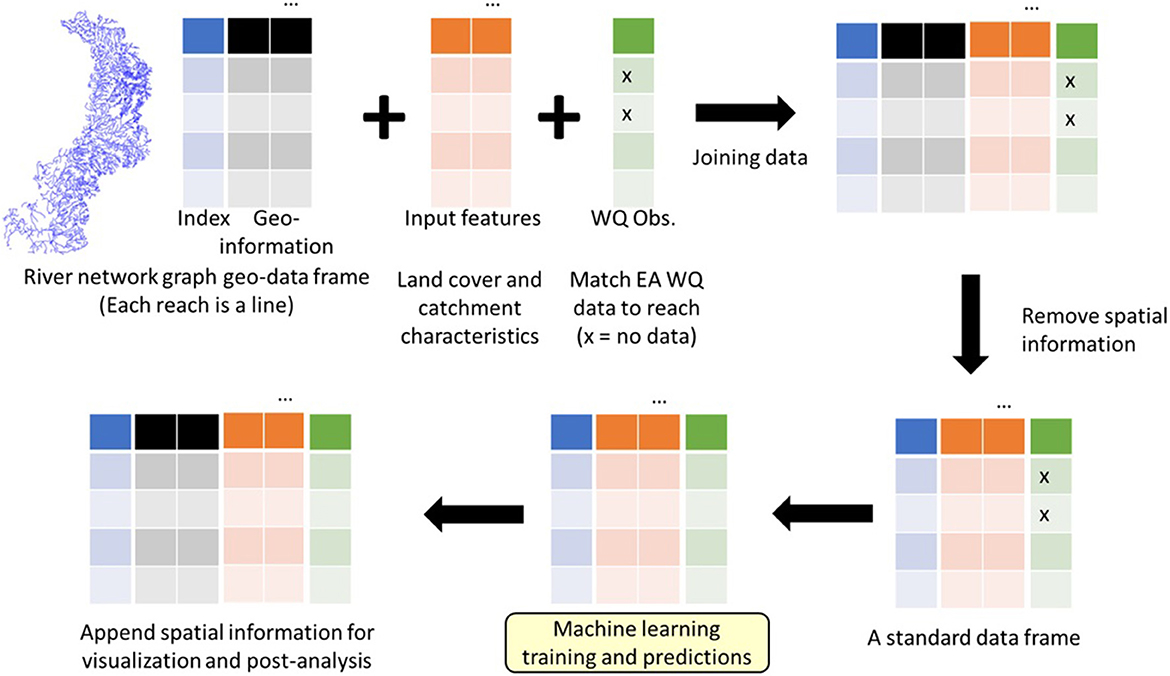
Figure 1. Overall framework for river reach-level machine learning predictions of water quality. Note that this framework is statistics-free and only involves the joining of data frames. It includes the following steps: (1) Input features and water quality observations are first matched to river reaches. (2) Spatial information is then removed to obtain a standard data frame so that standard machine learning methods can be used. (3) The spatial information is appended to the results for visualisation and post-analysis.

Details of the data sources and machine learning methods used to demonstrate this method are given in the remainder of this section. Jupyter notebooks to reproduce our workflow in Python are available in Magee et al. (2023).

2.2. Data sources

2.2.1. High-resolution river network graph for the UK

In our study, we subdivided our analysis based on 107 UK hydrometric areas (National River Flow Archive, 2014). These 107 hydrometric areas were either integral catchments with a single outlet to the sea or tidal estuary, or they included several river catchments having topographical similarity with separate tidal outlets. We also used a UK reach-level river network digitised from OS mapping at a 1:50,000 scale (Fry et al., 2000). Canals and other artificial water bodies were removed, and the flow paths through lakes were represented by centrelines. Rivers stretches contain connectivity information, but this was not explicitly made use of in this study. Most river stretches in the network represented the entire line between confluences and included bifurcations. The river network graph also included information such as length, identifier, and name of the parent river (for larger rivers), hydrometric area, and the Strahler and Shreve stream order for each reach.

2.2.2. UK Environment Agency (EA) water quality data

The Environment Agency maintains water quality monitoring data for a multitude of water sampling sites throughout England for a range of water body types from coastal or estuarine waters, rivers, lakes, ponds, canals, or ground waters in the Water Quality Archive (WQA, https://environment.data.gov.uk/water-quality/view/landing). Readings are taken for a variety of purposes, including compliance assessments against discharge permits, environmental monitoring, as well as investigations for pollution incidents. The WQA only contains complete samples where all analyses have been completed. The data analysed for this study was accessed on 23 June 2021.

We extracted the data from WQA for 2010–2020 for “orthophosphate, reactive as P” and “nitrate as N.” These datasets were further filtered to consider only sample material types from rivers or running surface water bodies. We then aggregated the data by taking the mean for each season for each year at each sampling location contained within the datasets (i.e., winter: December, January, and February; spring: March, April, and May; summer: June, July, and August; autumn: September, October, and November). Note that the typical sampling interval for nitrates and orthophosphates varies considerably but is roughly between biweekly and monthly. However, it is not uncommon that at some sites, there may be periods of more than 8 weeks between samples. To minimise the effects of outliers, we used only the middle 95% of the data. The modelling was performed on log-transformed nitrate and orthophosphate data.

2.2.3. Catchment descriptors and Land Cover Map

Unlike some of the studies mentioned earlier, we used physical descriptions of the catchment area to aid with predictions for the machine learning models in this study. The UK Centre for Ecology and Hydrology (CEH) develops and maintains a number of catchment descriptor datasets to inform its UK freshwater research. Catchment descriptors are available on a gridded representation of the UK at 50 m resolution—the CEH Integrated Hydrological Digital Terrain Model, IHDTM (Morris and Flavin, 1990), where the values for each cell represent the catchment upstream of that cell. Cells are connected using topographical information but also include information from mapped contours and the digital river network to ensure consistency where mapped surface water bodies are present. The Flood Estimation Handbook (FEH) provides a dataset of landform catchment descriptors for every grid cell with a catchment area > 0.5 km². Further catchment descriptors, including land cover fractions from the UK Land Cover Map 2015 (Rowland et al., 2017), are maintained and provided at the same scale by the National River Flow Archive. For this study, the FEH descriptors and catchment land cover statistics were extracted for each individual river reach within the digital river network. A representative IHDTM grid cell was identified for each reach as that closest to the 70th percentile by area of all grid cells intersecting with the reach river line to maximise the likelihood that the cell correctly lies on the river stretch. All catchment descriptors were from the raster datasets and stored alongside the river reach attributes.

The full list of FEH descriptors and land cover input features initially considered for machine learning algorithms are described in Table 1. The full and final features chosen for the final model are discussed in Section 3. The FEH descriptors were then matched to the river stretch ID for the Environment Agency's phosphate and nitrate readings.

TABLE 1

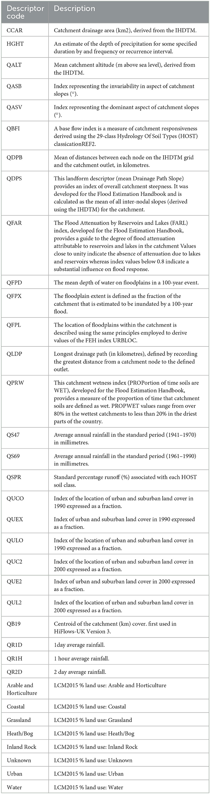
Table 1. Description of catchment descriptors used as input features for the construction of water quality machine learning models.

2.3. Training data, pre-processing, and feature engineering

After collating all data sources, the sample point IDs from the WQA were matched to the closest river stretch in the digital river network to integrate the two data sources. Note that this matching was a statistics-free process—all variables were matched to a river reach. As illustrated in Figure 1, all spatial information was excluded from the machine learning model and was not used in the post-analysis of results. Once the datasets were integrated, rows with missing data were excluded. The filtered nitrate and phosphate datasets contained 5,187 and 5,594 rows, respectively, for winter and a similar number of rows for other seasons. Once all missing values were removed, continuous features were normalised using min-max transformation. The reason for such a transformation is that large input values in a neural network can result in a model that learns large weights; models with large weight values are often unstable and may result in poor performance during learning, resulting in a higher generalisation error.

Min-max scaling was also chosen since it does not affect Pearson correlation scores between the potential features, helping with feature reduction in machine learning models. Feature reduction is a key part of data prepossessing, as reducing the dimensionality of a machine learning algorithm potentially reduces the execution time of machine learning algorithms, which is especially important for the tree-based algorithms implemented in this study. Irrelevant features within training data may also mislead the learning process of the final model, resulting in unexpected predictions. Including too many features may also result in overfitting of the model to the training data, resulting in poor predictions of new data (Kantardzic, 2019).

Highly correlated features can often be considered candidates for feature reduction, and the inclusion of highly correlated features provides little extra information from the data. Feature selection algorithms tend to fall within two categories: philtre and wrapper methods. Philtre methods rely on the general characteristics of the considered datasets to select features without involving the training of any machine learning methods. Therefore, this method is not affected by any inherent bias in the machine learning methods used. Wrapper methods, on the other hand, take up large amounts of processing time due to the training of many machine learning models (Kohavi and John, 1997). For this reason, a basic correlation philtre was applied to all continuous features. For each feature, the first feature that was correlated with an absolute value above 0.8 was removed from the datasets. The list of land cover and FEH descriptors with the descriptor codes that were used as input features are outlined in Table 1.

2.4. Seasonal nitrate and orthophosphate predictions

2.4.1. Random forest regressor for water quality modelling

Random forest models offer great flexibility and high predictive performance for environmental applications (e.g., Tyralis et al., 2019; Vergopolan et al., 2021). In this study, we trained a random forest (RF) model (Ho, 1995; Breiman, 2001) to predict either nitrate or orthophosphate levels for each season. Input features and water quality observations were matched to river reaches. The data were then used for training and predictions in the RF model. The final results were matched back to the river reaches. Fitting different models for each season and each chemical species allowed the RF models to select the most relevant input features for the given data.

The RF models are ensemble learners for classification and regression tasks. Ensemble methods use multiple weak learners to obtain a better predictive performance than using any of the constituent learning algorithms alone (Zhang, 2012). Ensemble learners such as RF models always converge by the strong law of large numbers and provide a distinct advantage over single decision trees, as overfitting is not as large of a problem (Ho, 1995; Breiman, 2001). To generate each tree in this ensemble method, bagging is often utilised. Bagging, also referred to as bootstrap aggregation, works as follows: given an initial training dataset D of size N, bagging generates new training sets D_i, each of size n by random sampling with replacement. Should N = n, then for large n, the set of training data in D_i is expected to have the fraction 1 − 1/e ~ 63% of the unique examples of D, with the rest being duplicates (Aslam et al., 2007). Sampling with replacement ensures that each bootstrap is independent of other bootstrapped samples since it does not depend on the previously chosen samples when sampling. For each training dataset D_i, a tree is trained, and the tree's outputs are combined, usually as an average of all tree outputs or as a voting system for classification. Bagging reduces variance and hence limits overfitting; however, unlike single trees, bagging and ensemble learners lose interpretability. Moreover, sampling and generation of many learners to produce suitable bagging ensemble models can be computationally expensive. RF models can also benefit from randomisation of features where a random subset of features is considered for splitting at each node. Boosting and the ability to consider random subsets for splitting tree nodes decreases the variance of the RF estimator. Moreover, for regression tasks, by taking an average of tree predictions, errors within single trees can be mitigated with a large number of estimators.

To obtain the optimal RF model, we tested each RF model with combinations of hyperparameters, which are listed in Table 2. We have reported only the results from RF methods in this study. For a comparison of the performance of different machine learning methods, see the preliminary study of Huxley (2021).

TABLE 2

Table 2. The combination of hyper-parameters tested to optimise the random forest model in a random grid search.

2.4.2. Feature importance and selection

To avoid overfitting, we performed a two-step procedure to select input features for the final RF models. First, we ran full RF models with all available features and ranked the features by descending importance values. Subsequently, the list of features was iterated by adding one feature at a time and calculating the variance inflation factor (VIF), which is defined as VIF = 1/(1 − R²), where R² is the coefficient of determination between two feature pairs. If the inclusion of the feature caused the VIF to exceed 10, then the feature was dropped. Otherwise, the feature was retained.

2.4.3. Cross-validation

It is not recommended to train a model on the same data it will be tested on since machine learning models tend to overfit the training data (Srivastava et al., 2014). Machine learning algorithms should be developed to maximise predictive accuracy on new data, not necessarily the training data. Fixation on fitting the best fit on training data will fit its noise by memorising its peculiarities rather than finding a general predictive rule (i.e., overfitting; Dietterich, 1995). To analyse whether a machine learning model is overfitted to the training data, we can use cross-validation and assess the performance of a machine learning algorithm on separate testing datasets.

To implement a random grid search, each nitrate and orthophosphate dataset was split into a training and a testing set. This was done by randomly assigning data points to the sets, with each testing set comprising 25% of the original dataset and the training sets with the remaining. The grid search was performed on the testing sets with k-fold cross-validation where k = 4. In k-fold validation, data is partitioned into k-equal or nearly equal sets using a stratification process or randomisation. Training and testing are performed on these partitioned sets, referred to as folds, in k iterations such that at each iteration, we leave 1-fold out for testing the trained model, where the remaining k-1 folds are used for training (Yadav and Shukla, 2016). The performance of the machine learning algorithm is determined by the mean of the metric scores of the k iterations. It has been shown for classification problems that k-fold validation provides a good indicator of model performance for large datasets. This is despite a trade-off between the number of cross-validation folds and the computation time for evaluating metrics, where more folds lead to increased computation time (Yadav and Shukla, 2016). K-fold validation is selected over other validation techniques, such as “hold one out,” mainly due to time and computational restraints. “Hold one out” trains the model with the whole training set except a single point and tests with a single point. For a random grid search, this would have led to a longer search time for the best hyperparameters compared to a k-fold validation approach due to the greater number of models trained. Using the “hold one out” method with a large training set could also lead to the selection of a hyperparameter set that overfits, with more outlier trends being learnt that lead to a final model that generalises poorly to new data. Due to the number of folds and time trade-off, k = 3 folds were used in the random grid search for hyperparameters to reduce searching time. Once the hyperparameters were selected, final models, which included 3-folds as the final training data, were trained. The final performance was determined using metrics on a held-out testing dataset, as illustrated in the next section.

2.4.4. Performance evaluation

To evaluate the performance of our machine learning methods, we considered the mean squared error (MSE), Nash-Sutcliffe model efficiency coefficient (NSE; Nash and Sutcliffe, 1970), and the Kling-Gupta efficiency (KGE; Gupta et al., 2009). The mean squared error (MSE) is defined as:

$\begin{array}{ll}MSE={\displaystyle \sum _i^n}{(x_i-{\widehat{x}}_i)}^2/n& (1)\end{array}$

where x_i represents the observation and ${\widehat{x}}_i$ represents the predicted value for data (i). The Nash-Sutcliffe model efficiency coefficient (NSE) is defined as:

$\begin{array}{ll}NSE=1-\frac{{\displaystyle {\sum }_i^n}{(x_i-{\widehat{x}}_i)}^2}{{\displaystyle {\sum }_i^n}{(x_i-\overline{x_i})}^2}& (2)\end{array}$

where $\overline{x_i}$ represents the mean of observations. The Kling-Gupta efficiency (KGE) is defined as:

$\begin{array}{ll}KGE=1-\sqrt{{(r-1)}^2+{(\alpha -1)}^2+{(\beta -1)}^2}& (3)\end{array}$

where r is the linear correlation between observations and simulations, α is a measure of the variability error, and β is a bias term, which can also be written as:

$\begin{array}{ll}KGE=1-\sqrt{{(r-1)}^2+{(\frac{\widehat{\sigma }}{\sigma }-1)}^2+{(\frac{\widehat{\mu }}{\mu }-1)}^2}& (4)\end{array}$

where μ and σ correspond to the mean and standard deviation, respectively. When NSE = 1 and KGE = 1, it indicates perfect agreement between simulation and observations. When NSE = 0, it indicates that the mean of observations provides better estimates than simulations.

3. Results

3.1. Feature selections and predictions

As discussed in the methods section, we adopted a two-step approach to initially run full RF models with all features and then select a subset of the features to run the final RF models. Table 3 shows the features selected for the models for each water quality species and season. In all models, coastal and unknown land use had zero feature importance. The Flood Attenuation by Reservoirs and Lakes (FARL) index [QFAR], catchment wetness index [QPRW], as well as 1-day, 2-day, 1-h average rainfall [QR1D, QR1H, and QR2D] were not selected in any models. Arable and horticulture land use was an important feature of all nitrate models. While five or more catchment descriptors were selected as input features in all other models, only three and four of them were selected for the winter and autumn nitrate models, respectively. While all nitrate models did not select grassland as an input feature, it was included in three of the four orthophosphate models. For predicting orthophosphate in winter, fewer land use features were selected, while average annual rainfall [QS69] and arable and horticulture were selected instead.

TABLE 3

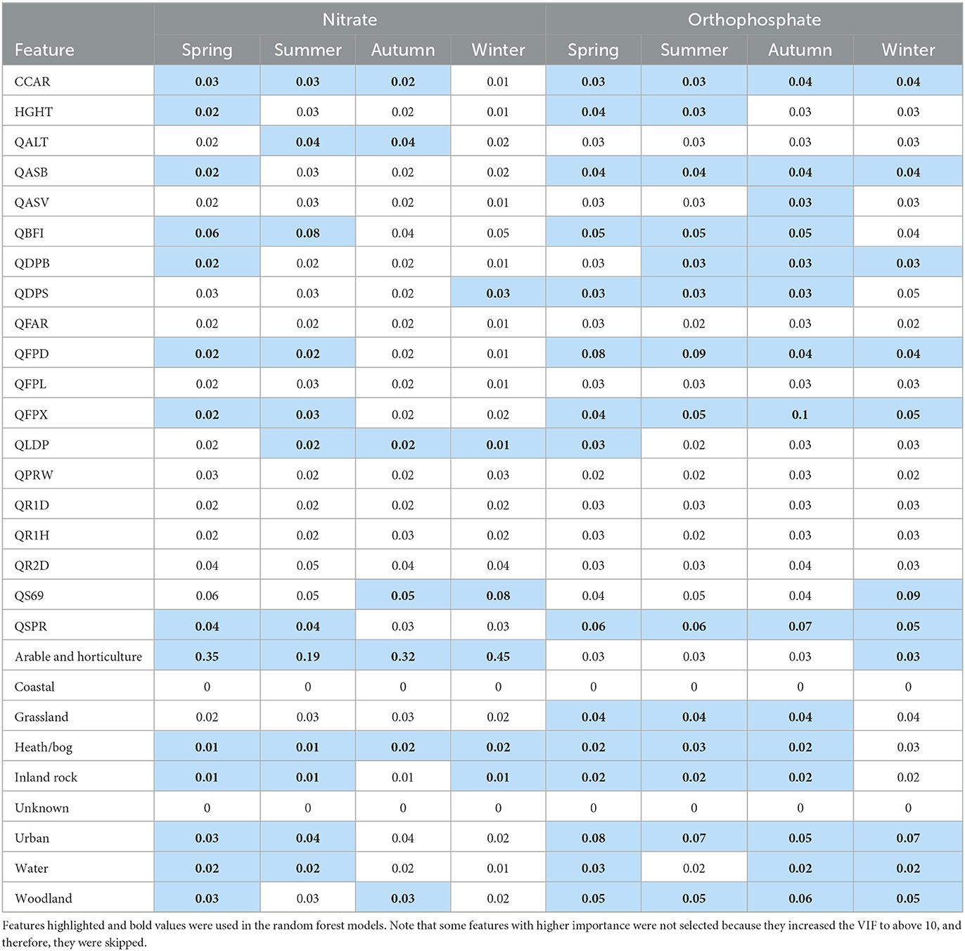
Table 3. Feature screening results.

The selected features listed in Table 3 were then used to run the final RF models and the final feature selection results are reported in Figure 2. For nitrate models, arable and horticulture land use was by far the most important input feature, while other land use features mostly had low importance. Catchment descriptors tended to have higher importance in autumn and winter, partly because fewer of them were selected in the previous stage. In the orthophosphate models, the contributions of feature importance were much more evenly distributed. The spring, summer, and autumn models were very similar, while the winter model had a rather different set of features, and their feature importance values were non-trivial. Specifically, the longest drainage length [QLDP], average annual rainfall [QS69], and arable and horticulture land use were included, while the baseflow index [QBFI], mean distance to catchment outlet [QDPB], and grassland were excluded. Catchment drainage area [CCAR], catchment slope invariability [QASB], mean depth of water and floodplain extent of a 100-year event [QFPD, QFPX], standard percentage runoff [QSPR], and urban and woodland land use were included in all orthophosphate models.

FIGURE 2

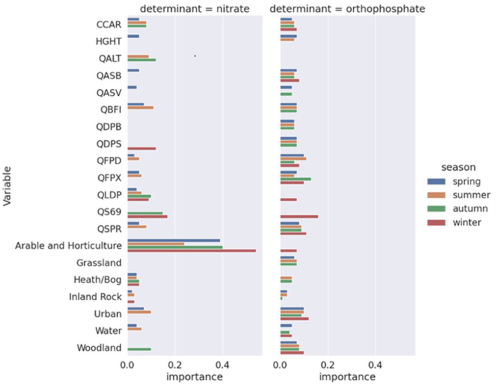
Figure 2. Final feature selection results of the random forest models. Note that features with zero importance are not included in the final models.

3.2. Overall model performance

3.2.1. Nitrate models

Once the predictions of nitrate concentrations were made by the RF model at each river reach, they were mapped back to the river network graph. Figure 3 shows the long-term predicted nitrate levels at each river reach in GB for each season. Central and eastern England were predicted to have higher nitrate concentrations, and they are higher in winter and spring than in summer and autumn. The exception was the Pennines, which had a low nitrate concentration that may be attributed to its topography, lower-intensity land use, lack of sewage inputs, and low base flow index. In Scotland and northern England, higher nitrate concentrations were mostly observed on the East Coast alone. While in some cases, small streams in remote areas had higher nitrate concentrations, in general, nitrate concentrations were higher in bigger streams.

FIGURE 3

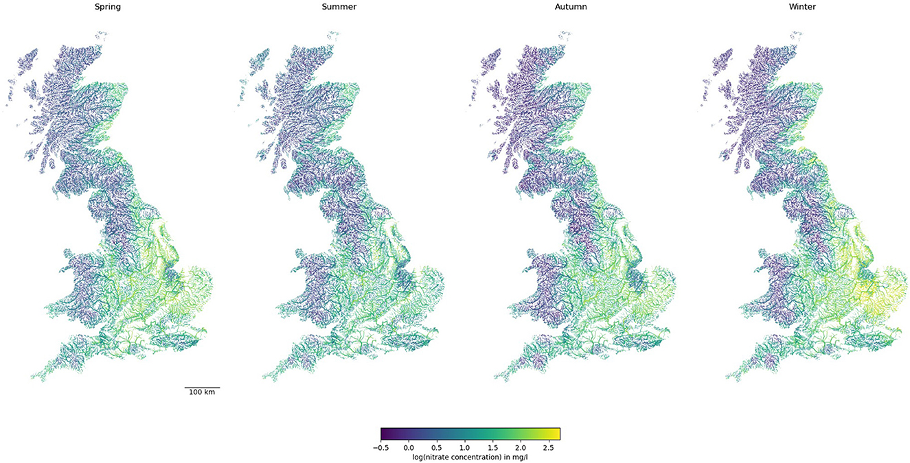
Figure 3. Predictions of nitrate concentration in rivers across GB. Note line widths are proportional to Strahler stream order (i.e., thicker for larger streams downstream).

Figures 5A, B illustrate the nitrate model performance in training and testing. For brevity, we grouped the results from all seasons together. The training data achieved a very good R² value of 0.96 (NSE of 0.91 and KGE of 0.83), and there was a very high density along the 1:1 line. It was also obvious from the Hexbin plot that nitrate observations were mostly concentrated between 1.0 and 2.0 of the log-transformed data, and there was a long tail for concentrations below 1.0.

There is evidence that the nitrate RF model exhibited slight overfitting as the training MSE of 0.25 (NSE of 0.51 and KGE of 0.61) was not as good as the testing MSE. However, its R² value of 0.71 was good, and despite some spread, the scatter points fell along the 1:1 line well.

Spatially, Figure 6 and Table 4 show that the nitrate RF model performed well and better generalised the whole of England based on testing the MSE values for each hydrometric area (HA, see Supplementary Figure 1). The RF models, on average, showed the larger HAs, and those not along the south and northeast coasts made better predictions and showed more consistent performance. The NSEs of many HAs reported a good value of 0.3 or above. A few HAs reported negative NSEs, indicating they had issues reproducing the mean. These were small Has, so their small sample size can be attributed to the NSE value, and it is not an indication of the model's predictive power in general. For KGE, better-than-average performances were observed in Tweed (HA = 21) and the HAs on the southwest coast.

TABLE 4

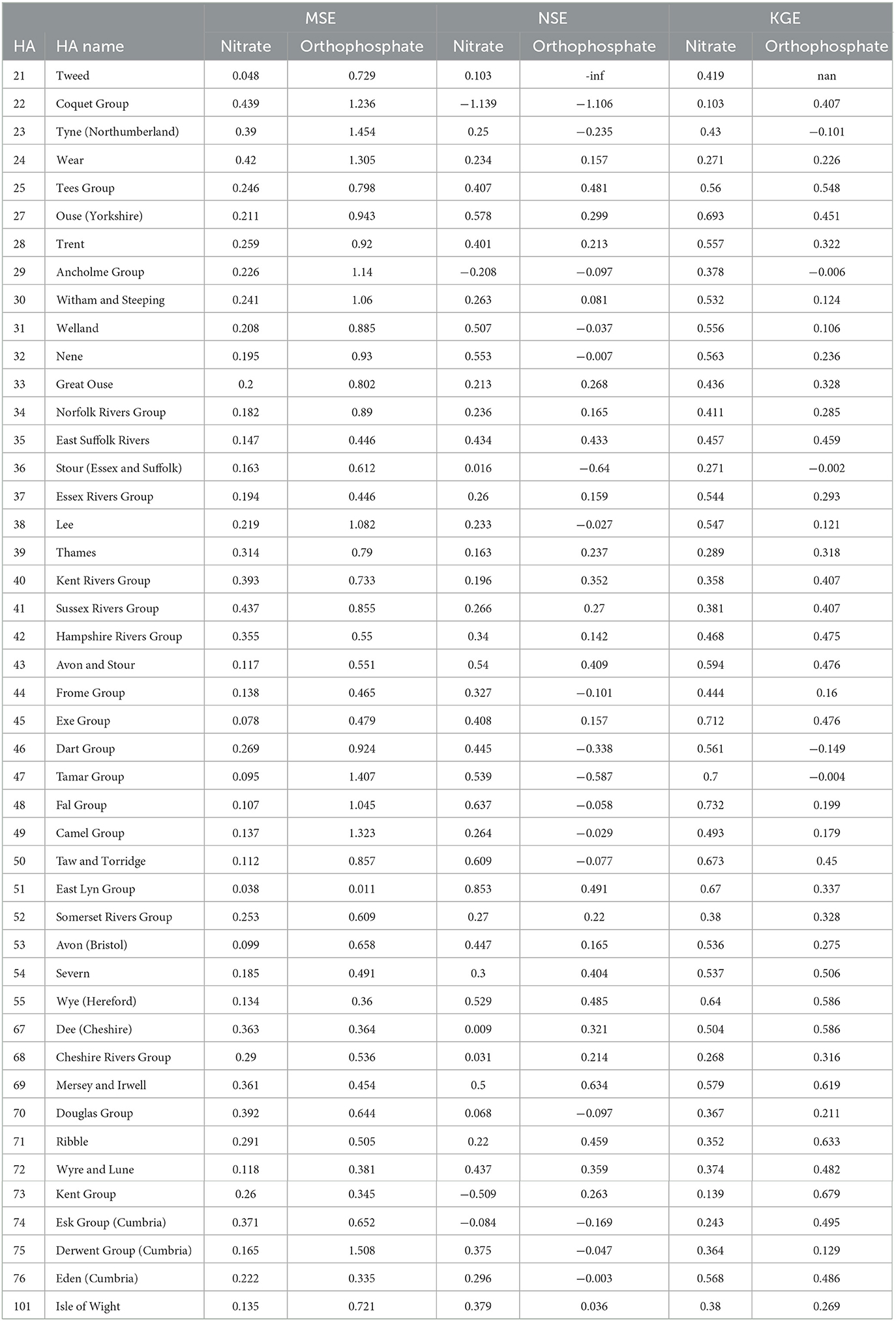
Table 4. Model performance metrics based on hydrometric areas (HAs) in England.

Based on the MSE, the nitrate RF models performed better on river reaches with a Strahler stream order 4–7 (Table 5) than lower-order streams. Based on the NSE and KGE, streams of orders 5 and 6 outperformed other streams. In particular, based on the NSE, the performance of order 1 and 7 streams were very similar. This indicated that nitrate predictions were more challenging for small streams and very large streams (order = 7), with the latter only having a few occurrences in the UK river network graph.

TABLE 5

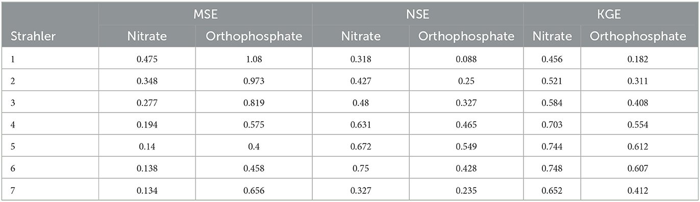
Table 5. Model performance metrics based on the Strahler stream order.

Figure 3 shows only subtle changes in nitrate levels between any two seasons. While nitrate levels between seasons are well-correlated, considerable variability within +/– 0.5 order of magnitude exists (Supplementary Figure 2A). This highlighted that with good training and cross-validation results for the models for each season (Figure 5), applying machine learning methods for nitrate predictions in every reach of the UK river network could lead to greater variability in predictions.

3.2.2. Orthophosphate models

Figure 4 illustrates the long-term predicted orthophosphate levels at each river reach in GB for each season. Similar to nitrate, central and eastern England had higher orthophosphate levels, but regions with high orthophosphate levels appeared to be smaller. Unlike nitrate levels, orthophosphate levels were higher in summer and autumn than in spring and winter.

FIGURE 4

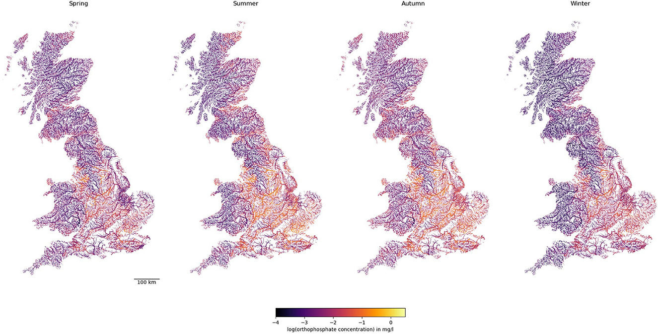
Figure 4. Predicted concentrations of orthophosphate in rivers across GB. Note line widths are proportional to Strahler stream order (i.e., thicker for larger streams downstream).

Figure 5 shows the orthophosphate model's performance in training and testing. The training data achieved a good R² value of 0.95 (NSE of 0.88 and KGE of 0.77), and there was a very high density along the 1:1 line. Furthermore, unlike nitrate, the Hexbin plot for orthophosphate did not show a skewed distribution. Some bias was noticeable in the predictions; the slope of the best-fit line was slightly steeper than the 1:1 line, indicating predicted values were higher than observed for high orthophosphate levels, while the opposite was true for low orthophosphate levels.

FIGURE 5

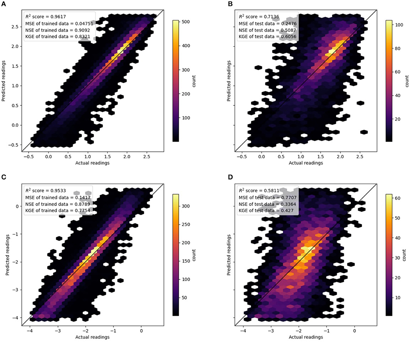
Figure 5. Hexbin plots showing the performance of random forest models. Note that models from the four seasons are plotted on a single plot. (A) Nitrate. Training data. (B) Nitrate. Testing data. (C) Orthophosphate. Training data. (D) Orthophosphate. Testing data.

There is evidence that the orthophosphate RF models exhibited slight overfitting as the training MSE of 0.77 (NSE of 0.33 and KGE of 0.43) was not as good as the testing MSE. Despite a rather large spread of the scatter points, the R² value of 0.77 indicated a good correlation between the predicted and observed data.

Overall, Figure 6 and Table 4 demonstrate that the orthophosphate RF models performed well and better generalised the whole of England based on the testing MSE values for each HA. The RF models, on rage, registered lower MSE at larger HAs and in the west of England (excluding the southwest coasts). The NSE of many HAs reported negative values, indicating they had issues reproducing the mean, which we partly observed in the Hexbin plots in Figure 5. For KGE, good performance (KGE > 0.5) could be observed in the Tees group (HA = 25), Severn (HA = 54), Wye (Hereford; HA = 55), Dee (Cheshire; HA = 67), Ribble (HA = 71), and Kent group (HA = 73), with many other HAs achieving similar performance. Meanwhile, Tyne (Northumberland; HA = 23) and Dart group (HA = 46) performed poorly (KGE < 0.1).

FIGURE 6

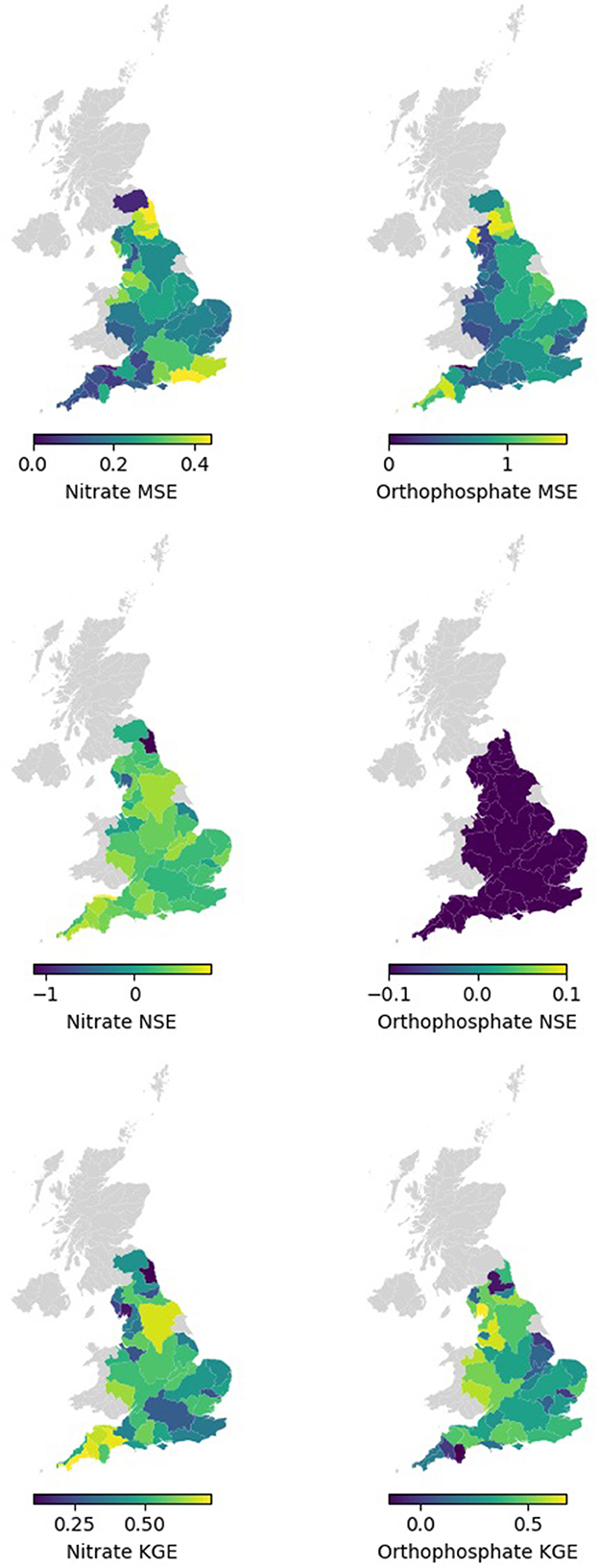
Figure 6. Spatial map of mean MSE, NSE, and KGE by hydrometric areas for testing data for nitrate, and orthophosphate.

Identical to the results for nitrate, the orthophosphate RF models performed better on river reaches with a Strahler stream order 4–7 (Table 5) than lower-order streams based on MSE. Based on NSE and KGE, streams of order 5 and 6 outperformed other streams. Again, this indicated that the orthophosphate predictions were more challenging for small streams and very large streams (order = 7).

Supplementary Figure 2B shows a scatter plot of predicted nitrate against orthophosphate at each river reaches in spring. It shows that despite some higher correlations in high nitrate-high orthophosphate conditions and at high Strahler stream order (6 or above), nitrate and orthophosphate levels were not well-correlated. This highlighted the differences in sources for nitrate and orthophosphate and in their sensitivity to input features. This also suggested that nitrate and orthophosphate may not be suitable to be used as a proxy measurement for each other.

3.3. Results from selected catchments

It can be difficult to visualise the nitrate and orthophosphate prediction at individual river reaches when all the river reaches of GB are presented in the same plot. Therefore, we focused on the results of four selected hydrometric areas in Figure 7. In Tweed (HA = 21), we observed much higher nitrate concentrations in streams in the east of the HA in winter. However, it caused just a small increase in nitrate concentration in its main river channel (i.e., River Tweed). Orthophosphate levels in the Tweed were generally very low; however, their levels were higher in smaller streams in summer and autumn. In the Thames (HA = 39) area, higher nitrate levels were observed in River Mole in the southeast of the HA, while higher orthophosphate levels tended to occur in smaller tributaries in the northwest of the HA. We observed slightly higher nitrate in spring and winter than in summer and autumn. There were a few localised orthophosphate hotspots in summer and autumn, causing some increase in orthophosphate in the Thames. In Wye (Hereford; HA = 55), nitrate levels were generally seasonally invariant. Obvious increases in orthophosphate in small streams near Hereford in summer and autumn were observed. However, it did not lead to a change in the very low orthophosphate levels in its 6th order streams—River Wye and River Monnow. For the Tay (HA = 15) in Scotland (note that all training data is from England), we observed very low nitrate levels in most of the HAs. These were slightly higher in the larger streams, and high levels were observed in the southeast corner of the HAs, which were slightly higher in spring and winter. Orthophosphate levels were also very low for most of the HAs. Slightly higher levels were observed in very small streams and some streams in the southeast corner of the HAs, while higher orthophosphate levels were observed in summer and autumn.

FIGURE 7

Figure 7. Nitrate and orthophosphate prediction results at (A) Tweed (HA = 21), (B) Thames (HA = 39), (C) Wye (Hereford; HA = 55), and (D) Tay (HA = 15). Note line widths are proportional to Strahler stream order (i.e., thicker for larger streams downstream). The maps on the right overlay the spring nitrate predictions on a UK map. In the right column, spring nitrate results are overlaid on a base map. To view results from other HAs, go to the following web application: https://moisture-wqmlviewer.datalabs.ceh.ac.uk/wqml_viewer.

4. Discussion

4.1. Key findings

We presented a flexible modelling framework that mapped point observations of river water quality of more than 200,000 river reaches across GB using machine learning. Our key findings are as follows:

• Model skill: The modelling approach we developed was able to estimate nitrate and orthophosphate levels with higher skill than existing statistical modelling approaches (Rothwell et al., 2010). A testing R² of 0.71 and 0.58, was attained for nitrate and orthophosphate, respectively.

• Flexibility: Our modelling approach is highly flexible. After matching the input features and observations to the river reaches, they could be used to build machine learning models without geographical or network information. This meant that input datasets required no modifications for commonly used machine learning methods to be applied. After the machine learning predictions are made, they can be mapped back to the river network (Section 2.1). Therefore, our method is applicable in all situations where (i) a high-resolution river network graph is available and (ii) input features and observations can be mapped to the graph. Features that were not considered in this study can be easily incorporated.

• Stream order: Plotting river-reach concentration predictions with stream order information is highly informative as it allows the visualisation of the evolution of nutrient levels downstream. Further, our model performs better with streams with higher Strathler stream order. This may be due to challenges in accurately linking catchment and land cover attributes to small streams with fewer observations.

The ability to estimate water quality at every point in a river network [based on the models of everywhere concept (Beven and Alcock, 2012; Blair et al., 2019)] has huge potential to revolutionise environmental science. For example, the chemical levels or other properties at any point in the river network can be queried, the effects along reaches on downstream biodiversity can be studied, and the cumulative exposure to a chemical to an organism can be calculated based on their trajectory in a simple and straightforward manner.

4.2. Drivers for water quality variability in the GB river network

Predicting river water quality using catchment characteristics (Davies and Neal, 2004, 2007; Rothwell et al., 2010; Oehler and Elliott, 2011; Lintern et al., 2018) and land use (Jarvie et al., 2008; Hutchins et al., 2010; Worrall et al., 2012) has been common practise. However, existing methods rely on multi-linear relationships between these characteristics and water quality, and they have rarely been applied at the national level. Furthermore, previous catchment characteristics and land use attributes are not matched at a fine scale. Similar to the findings by Rothwell et al. (2010), we found nitrate concentrations in UK rivers highly linked to agricultural land use, while diffuse and point sources (Bowes et al., 2008, 2009) tended to play a major role in orthophosphate concentrations. This was because household sources dominate P loads in many of GB's waters near high population density (White and Hammond, 2009).

4.3. Challenges, limitations, and future work

It is important to note that in this study, machine learning predictions were made at each river reach without any reference to their spatial location or connectivity. The land cover and catchment descriptors of each river reach were used as input features in a non-spatial way, and the resultant predictions were mapped back on the river network graph. This offered a very flexible approach to convert point observations of river water quality to maps at the relevant spatial scale (i.e., river reach). This method could be applied to other chemical species or geographical regions. Future studies could also investigate the method's applicability to river biodiversity indicators such as macroinvertebrate abundance (Powell et al., 2022).

A trade-off for the ease of use of our framework was that we did not make explicit assumptions on geostatistics based on distance or connectivity. However, as emerging approaches such as graph neural networks (Sun et al., 2022) or graph Gaussian processes (Pinder et al., 2022) have highlighted the importance of the connectivity of networks and provided more flexible tools to model them, future studies can extend our framework to include geostatistics or network connectivity.

Our study focused on the use of static input features for long-term predictions of water quality. An opposite group of approaches used very high temporal resolution driving data and sparse water quality data, as well as methods such as Long Short-term Memory (LSTM) to model the dynamics of water quality variations at chemically ungauged basins (Zhi et al., 2021). Future studies can consider both static and dynamic input features to obtain predictions that capture spatial trends and temporal variations.

Many physical processes that control the distribution and evolution of nitrate and orthophosphate are not explicitly considered in our study. For instance, the long-term evolution of these chemical species (Bell et al., 2021), the migration of nitrate from land surface to groundwater and its storage in the vadose zone (Wang et al., 2016; Ascott et al., 2017), or the discharge from sewage treatment works (Jarvie et al., 2006; Bowes et al., 2010) have not been explicitly considered. Future studies can also strive to improve the joint use and interpretation of process-based and machine learning water quality model results.

Because of the flexibility of the methods described in this study, they can potentially be applied elsewhere in the world or with different input variables. The water quality portal (Read et al., 2017) in the United States and the Global River Water Quality Archive (Virro et al., 2021) are examples of other centralised databases for water quality measurements where the models from this study can be applied. The availability of global high-resolution river network graphs makes it possible to repeat a similar analysis globally (Linke et al., 2019; Yan et al., 2022). However, if the use of river reach characteristics that are not provided in those graphs is required, users need to match those characteristics to the graphs. For GB, CAMELS-GB (Coxon et al., 2020) may be a richer, alternative dataset that can be matched to the river network graph for an analysis similar to the one presented in this study. Future studies can also compare river network water quality predictions with remote sensing of water quality for inland waters, such as those obtained from AquaSat (Ross et al., 2019).

Finally, the proposed framework may be applied iteratively to optimise the design of water quality monitoring networks. It can be used to design the placement of new point sampling locations or to assess the information content of sampling locations by comparing the resultant reach scale water quality maps.

5. Conclusion

Current methods for water quality mapping are often conducted at a grid-based level, masking the important sense of network connectivity that is intrinsic to rivers. This limits their utility to inform policy and decision-making. While some methods have been developed for mapping river quality in networks, they are often not readily applicable at a national scale.

With the advancement of machine learning and very high-resolution river graphs becoming available at national levels, it becomes possible to map the spatial variability of water quality variables nationally. To our knowledge, this study is the first to predict water quality at each river reach nationally for Great Britain. Our study builds on previous approaches by integrating static variables into seasonal water quality prediction and by demonstrating the use of machine learning to effectively make water quality predictions without the need to specify geostatistical constraints. Mapping the water quality of every British river reach also has the potential to serve as a new fit-for-purpose tool when evaluating the water quality in British rivers (Whelan et al., 2022).

By demonstrating a practical way to map water quality monitoring data from a network of stations to river reaches in an entire country, this study provides a way for reach-scale interrogation of water quality data in decision-making, which allows much more targeted actions to improve and protect water quality in rivers.

Data availability statement

The data presented in the study are deposited in the Environmental Information Data Centre, accession number https://doi.org/10.5285/ba208b6c-6f1a-43b1-867d-bc1adaff6445.

Author contributions

C-HT: conceptualisation, software, visualisation, and writing—original draught preparation. EM: formal analysis, investigation, and software. DH: methodology, investigation, and software. ME: methodology. MF: conceptualisation, data curation, methodology, resources, and supervision. All authors: writing—reviewing and editing. All authors contributed to the article and approved the submitted version.

Funding

This work was part of the UK-SCAPE: UK Status, Change and Projections of the Environment project, a National Capability award funded by the UK Natural Environmental Research Council (NERC: NE/R016429/1).

Acknowledgments

This study was developed during DH's summer placement at UKCEH as part of his M.Sc. in Data Science dissertation at Lancaster University. We thank Mike Bowes (UKCEH) for his helpful feedback on the manuscript.

Conflict of interest

The authors declare that the research was conducted in the absence of any commercial or financial relationships that could be construed as a potential conflict of interest.

Publisher's note

All claims expressed in this article are solely those of the authors and do not necessarily represent those of their affiliated organizations, or those of the publisher, the editors and the reviewers. Any product that may be evaluated in this article, or claim that may be made by its manufacturer, is not guaranteed or endorsed by the publisher.

Supplementary material

The Supplementary Material for this article can be found online at: https://www.frontiersin.org/articles/10.3389/frwa.2023.1244024/full#supplementary-material

References

Ahmed, U., Mumtaz, R., Anwar, H., Shah, A. A., Irfan, R., and García-Nieto, J. (2019). Efficient water quality prediction using supervised machine learning. Water 11, 2210. doi: 10.3390/w11112210

PubMed Abstract | CrossRef Full Text | Google Scholar

Ascott, M. J., Gooddy, D. C., Wang, L., Stuart, M. E., Lewis, M. A., Ward, R. S., et al. (2017). Global patterns of nitrate storage in the vadose zone. Nat. Commun. 8, 1416. doi: 10.1038/s41467-017-01321-w

PubMed Abstract | CrossRef Full Text | Google Scholar

Aslam, J. A., Popa, R. A., and Rivest, R. L. (2007). “On estimating the size and confidence of a statistical audit,” in Proceedings of the USENIX Workshop on Accurate Electronic Voting Technology, EVT'07 (Philadelphia, PA: USENIX Association), 8.

Google Scholar

Bell, V. A., Naden, P. S., Tipping, E., Davies, H. N., Carnell, E., Davies, J. A. C., et al. (2021). Long term simulations of macronutrients (C, N and P) in UK freshwaters. Sci. Total Environ. 776, 145813. doi: 10.1016/j.scitotenv.2021.145813

CrossRef Full Text | Google Scholar

Beven, K. J., and Alcock, R. E. (2012). Modelling everything everywhere: a new approach to decision-making for water management under uncertainty. Freshw. Biol. 57, 124–132. doi: 10.1111/j.1365-2427.2011.02592.x

CrossRef Full Text | Google Scholar

Bhattarai, A., Dhakal, S., Gautam, Y., and Bhattarai, R. (2021). Prediction of nitrate and phosphorus concentrations using machine learning algorithms in watersheds with different landuse. Water 13, 3096. doi: 10.3390/w13213096

CrossRef Full Text | Google Scholar

Blair, G. S., Beven, K., Lamb, R., Bassett, R., Cauwenberghs, K., Hankin, B., et al. (2019). Models of everywhere revisited: a technological perspective. Environ. Model. Softw. 122, 104521. doi: 10.1016/j.envsoft.2019.104521

CrossRef Full Text | Google Scholar

Bowes, M. J., Neal, C., Jarvie, H. P., Smith, J. T., and Davies, H. N. (2010). Predicting phosphorus concentrations in British rivers resulting from the introduction of improved phosphorus removal from sewage effluent. Sci. Total Environ. 408, 4239–4250. doi: 10.1016/j.scitotenv.2010.05.016

PubMed Abstract | CrossRef Full Text | Google Scholar

Bowes, M. J., Smith, J. T., Jarvie, H. P., and Neal, C. (2008). Modelling of phosphorus inputs to rivers from diffuse and point sources. Sci. Total Environ. 395, 125–138. doi: 10.1016/j.scitotenv.2008.01.054

PubMed Abstract | CrossRef Full Text | Google Scholar

Bowes, M. J., Smith, J. T., Jarvie, H. P., Neal, C., and Barden, R. (2009). Changes in point and diffuse source phosphorus inputs to the River Frome (Dorset, UK) from 1966 to 2006. Sci. Total Environ. 407, 1954–1966. doi: 10.1016/j.scitotenv.2008.11.026

PubMed Abstract | CrossRef Full Text | Google Scholar

Breiman, L. (2001). Random forests. Mach. Learn. 45, 5–32. doi: 10.1023/A:1010933404324

CrossRef Full Text | Google Scholar

Comber, S. D. W., Smith, R., Daldorph, P., Gardner, M. J., Constantino, C., and Ellor, B. (2013). Development of a chemical source apportionment decision support framework for catchment management. Environ. Sci. Technol. 47, 9824–9832. doi: 10.1021/es401793e

PubMed Abstract | CrossRef Full Text | Google Scholar

Coxon, G., Addor, N., Bloomfield, J. P., Freer, J., Fry, M., Hannaford, J., et al. (2020). CAMELS-GB: hydrometeorological time series and landscape attributes for 671 catchments in Great Britain. Earth Syst. Sci. Data 12, 2459–2483. doi: 10.5194/essd-12-2459-2020

CrossRef Full Text | Google Scholar

Davies, H., and Neal, C. (2004). GIS-based methodologies for assessing nitrate, nitrite and ammonium distributions across a major UK basin, the Humber. Hydrol. Earth Syst. Sci. 8, 823–833. doi: 10.5194/hess-8-823-2004

CrossRef Full Text | Google Scholar

Davies, H., and Neal, C. (2007). Estimating nutrient concentrations from catchment characteristics across the UK. Hydrol. Earth Syst. Sci. 11, 550–558. doi: 10.5194/hess-11-550-2007

CrossRef Full Text | Google Scholar

Demir, I., and Szczepanek, R. (2017). Optimization of river network representation data models for web-based systems. Earth Sp. Sci. 4, 336–347. doi: 10.1002/2016EA000224

CrossRef Full Text | Google Scholar

Dietterich, T. (1995). Overfitting and undercomputing in machine learning. ACM Comput. Surv. 27, 326–327. doi: 10.1145/212094.212114

CrossRef Full Text | Google Scholar

Evans, C. D., Cooper, D. M., Juggins, S., Jenkins, A., and Norris, D. (2006). A linked spatial and temporal model of the chemical and biological status of a large, acid-sensitive river network. Sci. Total Environ. 365, 167–185. doi: 10.1016/j.scitotenv.2006.02.037

PubMed Abstract | CrossRef Full Text | Google Scholar

Frei, R. J., Lawson, G. M., Norris, A. J., Cano, G., Vargas, M. C., Kujanpää, E., et al. (2021). Limited progress in nutrient pollution in the U.S. caused by spatially persistent nutrient sources. PLoS ONE 16, e0258952. doi: 10.1371/journal.pone.0258952

PubMed Abstract | CrossRef Full Text | Google Scholar

Fry, M., Moore, R. V., Morris, D. G., and Flavin, R. W. (2000). UKCEH Digital River Network of Great Britain (1:50,000). Available online at: https://catalogue.ceh.ac.uk/documents/7d5e42b6-7729-46c8-99e9-f9e4efddde1d

Google Scholar

Giachetta, E., and Willett, S. D. (2018). A global dataset of river network geometry. Sci. Data 5, 180127. doi: 10.1038/sdata.2018.127

PubMed Abstract | CrossRef Full Text | Google Scholar

Granata, F., Papirio, S., Esposito, G., Gargano, R., and De Marinis, G. (2017). Machine learning algorithms for the forecasting of wastewater quality indicators. Water 9, 105. doi: 10.3390/w9020105

CrossRef Full Text | Google Scholar

Grizzetti, B., Bouraoui, F., de Marsily, G., and Bidoglio, G. (2005). A statistical method for source apportionment of riverine nitrogen loads. J. Hydrol. 304, 302–315. doi: 10.1016/j.jhydrol.2004.07.036

CrossRef Full Text | Google Scholar

Gupta, H. V., Kling, H., Yilmaz, K. K., and Martinez, G. F. (2009). Decomposition of the mean squared error and NSE performance criteria: implications for improving hydrological modelling. J. Hydrol. 377, 80–91. doi: 10.1016/j.jhydrol.2009.08.003

CrossRef Full Text | Google Scholar

Ho, T. K. (1995). “Random decision forests,” in Proceedings of 3rd International Conference on Document Analysis and Recognition (Montreal: IEEE Computer Society Press), 278–282.

Google Scholar

Howden, N. J. K., and Burt, T. P. (2009). Statistical analysis of nitrate concentrations from the Rivers Frome and Piddle (Dorset, UK) for the period 1965-2007. Ecohydrology 2, 55–65. doi: 10.1002/eco.39

CrossRef Full Text | Google Scholar

Hutchins, M. G., Deflandre-Vlandas, A., Posen, P. E., Davies, H. N., and Neal, C. (2010). How do river nitrate concentrations respond to changes in land-use? A modelling case study of headwaters in the River Derwent Catchment, North Yorkshire, UK. Environ. Model. Assess. 15, 93–109. doi: 10.1007/s10666-009-9218-2

CrossRef Full Text | Google Scholar

Huxley, D. (2021). Spatiotemporal Analysis of Nitrate and Phosphate in UK River Stretches Using Machine Learning. Lancaster: Lancaster University.

Google Scholar

Jarvie, H. P., Neal, C., and Withers, P. J. A. (2006). Sewage-effluent phosphorus: a greater risk to river eutrophication than agricultural phosphorus? Sci. Total Environ. 360, 246–253. doi: 10.1016/j.scitotenv.2005.08.038

PubMed Abstract | CrossRef Full Text | Google Scholar

Jarvie, H. P., Withers, P. J. A., Hodgkinson, R., Bates, A., Neal, M., Wickham, H. D., et al. (2008). Influence of rural land use on streamwater nutrients and their ecological significance. J. Hydrol. 350, 166–186. doi: 10.1016/j.jhydrol.2007.10.042

CrossRef Full Text | Google Scholar

Kantardzic, M. (2019). Data Mining: Concepts, Models, Methods, and Algorithms, 3rd Edn. Hoboken, NJ: Wiley-IEEE Press.

Google Scholar

Kohavi, R., and John, G. H. (1997). Wrappers for feature subset selection. Artif. Intell. 97, 273–324. doi: 10.1016/S0004-3702(97)00043-X

CrossRef Full Text | Google Scholar

Lane, R. A., and Kay, A. L. (2021). Climate change impact on the magnitude and timing of hydrological extremes across Great Britain. Front. Water 3, 684982. doi: 10.3389/frwa.2021.684982

CrossRef Full Text | Google Scholar

Lin, J., Compton, J. E., Hill, R. A., Herlihy, A. T., Sabo, R. D., Brooks, J. R., et al. (2021). Context is everything: interacting inputs and landscape characteristics control stream nitrogen. Environ. Sci. Technol. 55, 7890–7899. doi: 10.1021/acs.est.0c07102

PubMed Abstract | CrossRef Full Text | Google Scholar

Lin, P., Pan, M., Wood, E. F., Yamazaki, D., and Allen, G. H. (2021). A new vector-based global river network dataset accounting for variable drainage density. Sci. Data 8, 28. doi: 10.1038/s41597-021-00819-9

PubMed Abstract | CrossRef Full Text | Google Scholar

Linke, S., Lehner, B., Ouellet Dallaire, C., Ariwi, J., Grill, G., Anand, M., et al. (2019). Global hydro-environmental sub-basin and river reach characteristics at high spatial resolution. Sci. Data 6, 283. doi: 10.1038/s41597-019-0300-6

PubMed Abstract | CrossRef Full Text | Google Scholar

Lintern, A., Webb, J. A., Ryu, D., Liu, S., Waters, D., Leahy, P., et al. (2018). What are the key catchment characteristics affecting spatial differences in riverine water quality? Water Resour. Res. 54, 7252–7272. doi: 10.1029/2017WR022172

CrossRef Full Text | Google Scholar

Magee, E., Huxley, D., and Tso, C. M. (2023). Random Forest Model to Predict Long-Term Seasonal Nitrate and Orthophosphate Concentrations in British River Reaches. NERC EDS Environmental Information Data Centre. Available online at: https://catalogue.ceh.ac.uk/documents/ba208b6c-6f1a-43b1-867d-bc1adaff6445

Google Scholar

Morris, D. G., and Flavin, R. W. (1990). “A digital terrain model for hydrology,” in Proc 4th International Symposium on Spatial Data Handling (Zürich), 250–262.

Google Scholar

Morton, R., and Henderson, B. L. (2008). Estimation of nonlinear trends in water quality: an improved approach using generalized additive models. Water Resour. Res. 44. doi: 10.1029/2007WR006191

PubMed Abstract | CrossRef Full Text | Google Scholar

Mueller, N. D., Gerber, J. S., Johnston, M., Ray, D. K., Ramankutty, N., and Foley, J. A. (2012). Closing yield gaps through nutrient and water management. Nature 490, 254–257. doi: 10.1038/nature11420

PubMed Abstract | CrossRef Full Text | Google Scholar

Najah Ahmed, A., Binti Othman, F., Abdulmohsin Afan, H., Khaleel Ibrahim, R., Ming Fai, C., Shabbir Hossain, M., et al. (2019). Machine learning methods for better water quality prediction. J. Hydrol. 578, 124084. doi: 10.1016/j.jhydrol.2019.124084

CrossRef Full Text | Google Scholar

Nash, J. E., and Sutcliffe, J. V. (1970). River flow forecasting through conceptual models part I—a discussion of principles. J. Hydrol. 10, 282–290. doi: 10.1016/0022-1694(70)90255-6

CrossRef Full Text | Google Scholar

National River Flow Archive (2014). Hydrometric Areas for Great Britain and Northern Ireland. National River Flow Archive. Available online at: https://nrfa.ceh.ac.uk/

Google Scholar

O'Donnell, D., Rushworth, A., Bowman, A. W., Scott, E. M., and Hallard, M. (2014). Flexible regression models over river networks. J. R. Stat. Soc. Ser. C 63, 12024. doi: 10.1111/rssc.12024

PubMed Abstract | CrossRef Full Text | Google Scholar

Oehler, F., and Elliott, A. H. (2011). Predicting stream N and P concentrations from loads and catchment characteristics at regional scale: a concentration ratio method. Sci. Total Environ. 409, 5392–5402. doi: 10.1016/j.scitotenv.2011.08.025

PubMed Abstract | CrossRef Full Text | Google Scholar

O'Sullivan, C. M., Ghahramani, A., Deo, R. C., Pembleton, K., Khan, U., and Tuteja, N. (2022). Classification of catchments for nitrogen using Artificial Neural Network Pattern Recognition and spatial data. Sci. Total Environ. 809, 151139. doi: 10.1016/j.scitotenv.2021.151139

PubMed Abstract | CrossRef Full Text | Google Scholar

Pinder, T., Turnbull, K., Nemeth, C., and Leslie, D. (2022). “Street-level air pollution modelling with graph gaussian processes,” in ICLR: AI for Earth and Space Science.

Google Scholar

Powell, K. E., Oliver, T. H., Johns, T., González-Suárez, M., England, J., and Roy, D. B. (2022). Abundance trends for river macroinvertebrates vary across taxa, trophic group and river typology. Glob. Chang. Biol. 29, 1282–1295. doi: 10.1111/gcb.16549

PubMed Abstract | CrossRef Full Text | Google Scholar

Read, E. K., Carr, L., De Cicco, L., Dugan, H. A., Hanson, P. C., Hart, J. A., et al. (2017). Water quality data for national-scale aquatic research: the Water Quality Portal. Water Resour. Res. 53, 1735–1745. doi: 10.1002/2016WR019993

CrossRef Full Text | Google Scholar

Ross, M. R. V., Topp, S. N., Appling, A. P., Yang, X., Kuhn, C., Butman, D., et al. (2019). AquaSat: a data set to enable remote sensing of water quality for inland waters. Water Resour. Res. 55, 10012–10025. doi: 10.1029/2019WR024883

CrossRef Full Text | Google Scholar

Rothwell, J. J., Dise, N. B., Taylor, K. G., Allott, T. E. H., Scholefield, P., Davies, H., et al. (2010). Predicting river water quality across North West England using catchment characteristics. J. Hydrol. 395, 153–162. doi: 10.1016/j.jhydrol.2010.10.015

CrossRef Full Text | Google Scholar

Rowland, C. S., Morton, R. D., Carrasco, L., McShane, G., O'Neil, A. W., and Wood, C. M. (2017). Land Cover Map 2015 (1 km Percentage Aggregate Class, GB). NERC EDS Environmental Information Data Centre (Dataset). doi: 10.5285/7115bc48-3ab0-475d-84ae-fd3126c20984

CrossRef Full Text | Google Scholar

Sarker, S., Veremyev, A., Boginski, V., and Singh, A. (2019). Critical nodes in river networks. Sci. Rep. 9, 11178. doi: 10.1038/s41598-019-47292-4

PubMed Abstract | CrossRef Full Text | Google Scholar

Shen, L. Q., Amatulli, G., Sethi, T., Raymond, P., and Domisch, S. (2020). Estimating nitrogen and phosphorus concentrations in streams and rivers, within a machine learning framework. Sci. Data 7, 161. doi: 10.1038/s41597-020-0478-7

PubMed Abstract | CrossRef Full Text | Google Scholar

Smith, R. A., Schwarz, G. E., and Alexander, R. B. (1997). Regional interpretation of water-quality monitoring data. Water Resour. Res. 33, 2781–2798. doi: 10.1029/97WR02171

CrossRef Full Text | Google Scholar

Srivastava, N., Hinton, G., Krizhevsky, A., Sutskever, I., and Salakhutdinov, R. (2014). Dropout: a simple way to prevent neural networks from overfitting. J. Mach. Learn. Res. 15, 1929–1958.

PubMed Abstract | Google Scholar

Sun, A. Y., Jiang, P., Yang, Z.-L., Xie, Y., and Chen, X. (2022). A graph neural network approach to basin-scale river network learning: the role of physics-based connectivity and data fusion. Hydrol. Earth Syst. Sci. Discuss. 2022, 1–35. doi: 10.5194/hess-26-5163-2022

CrossRef Full Text | Google Scholar

Tyralis, H., Papacharalampous, G., and Langousis, A. (2019). A brief review of random forests for water scientists and practitioners and their recent history in water resources. Water 11, 910. doi: 10.3390/w11050910

CrossRef Full Text | Google Scholar

Vergopolan, N., Xiong, S., Estes, L., Wanders, N., Chaney, N. W., Wood, E. F., et al. (2021). Field-scale soil moisture bridges the spatial-scale gap between drought monitoring and agricultural yields. Hydrol. Earth Syst. Sci. 25, 1827–1847. doi: 10.5194/hess-25-1827-2021

CrossRef Full Text | Google Scholar

Virro, H., Amatulli, G., Kmoch, A., Shen, L., and Uuemaa, E. (2021). GRQA: global river water quality archive. Earth Syst. Sci. Data 13, 5483–5507. doi: 10.5194/essd-13-5483-2021

CrossRef Full Text | Google Scholar

Wang, L., Stuart, M. E., Lewis, M. A., Ward, R. S., Skirvin, D., Naden, P. S., et al. (2016). The changing trend in nitrate concentrations in major aquifers due to historical nitrate loading from agricultural land across England and Wales from 1925 to 2150. Sci. Total Environ. 542, 694–705. doi: 10.1016/j.scitotenv.2015.10.127

PubMed Abstract | CrossRef Full Text | Google Scholar

Whelan, M. J., Linstead, C., Worrall, F., Ormerod, S. J., Durance, I., Johnson, A. C., et al. (2022). Is water quality in British rivers “better than at any time since the end of the Industrial Revolution”? Sci. Total Environ. 843, 157014. doi: 10.1016/j.scitotenv.2022.157014

PubMed Abstract | CrossRef Full Text | Google Scholar

White, P. J., and Hammond, J. P. (2009). The sources of phosphorus in the waters of Great Britain. J. Environ. Qual. 38, 13–26. doi: 10.2134/jeq2007.0658

PubMed Abstract | CrossRef Full Text | Google Scholar

Whitehaed, P., Wilson, E., and Butterfield, D. (1998). A semi-distributed ntegrated itrogen model for multiple source assessment in tchments (INCA): part I—model structure and process equations. Sci. Total Environ. 210–211, 547–558. doi: 10.1016/S0048-9697(98)00037-0

CrossRef Full Text | Google Scholar

Worrall, F., Davies, H., Burt, T., Howden, N. J. K., Whelan, M. J., Bhogal, A., et al. (2012). The flux of dissolved nitrogen from the UK—evaluating the role of soils and land use. Sci. Total Environ. 434, 90–100. doi: 10.1016/j.scitotenv.2012.01.035

PubMed Abstract | CrossRef Full Text | Google Scholar

Xu, J., Xu, Z., Kuang, J., Lin, C., Xiao, L., Huang, X., et al. (2021). An alternative to laboratory testing: random forest-based water quality prediction framework for inland and nearshore water bodies. Water 13, 3262. doi: 10.3390/w13223262

CrossRef Full Text | Google Scholar

Yadav, S., and Shukla, S. (2016). “Analysis of k-fold cross-validation over hold-out validation on colossal datasets for quality classification,” in 2016 IEEE 6th International Conference on Advanced Computing (IACC) (Bhimavaram: IEEE), 78–83.

Google Scholar

Yan, D., Li, C., Zhang, X., Wang, J., Feng, J., Dong, B., et al. (2022). A data set of global river networks and corresponding water resources zones divisions v2. Sci. Data 9, 770. doi: 10.1038/s41597-022-01888-0

PubMed Abstract | CrossRef Full Text | Google Scholar

Yang, G., and Moyer, D. L. (2020). Estimation of nonlinear water-quality trends in high-frequency monitoring data. Sci. Total Environ. 715, 136686. doi: 10.1016/j.scitotenv.2020.136686

PubMed Abstract | CrossRef Full Text | Google Scholar

Zhang, C. (2012). Ensemble Machine Learning: Methods and Applications. New York, NY: Springer.

Google Scholar

Zhi, W., Feng, D., Tsai, W. P., Sterle, G., Harpold, A., Shen, C., et al. (2021). From hydrometeorology to river water quality: can a deep learning model predict dissolved oxygen at the continental scale? Environ. Sci. Technol. 55, 2357–2368. doi: 10.1021/acs.est.0c06783

PubMed Abstract | CrossRef Full Text | Google Scholar

Zounemat-Kermani, M., Batelaan, O., Fadaee, M., and Hinkelmann, R. (2021). Ensemble machine learning paradigms in hydrology: a review. J. Hydrol. 598, 126266. doi: 10.1016/j.jhydrol.2021.126266

CrossRef Full Text | Google Scholar