 Abdessamad Jari1*El Mostafa Bachaoui1
 Soufiane Hajaj1*Achraf Khaddari2Younes Khandouch3Abderrazak El Harti1Amine Jellouli1
 Mustapha Namous4
- 1Geomatics, Georesources and Environment Laboratory, Faculty of Sciences and Techniques, Sultan Moulay Slimane University, Beni Mellal, Morocco
- 2Laboratory of Geosciences, Department of Geology, Faculty of Sciences, Ibn Tofail University, Kenitra, Morocco
- 3Laboratory of Metrology and Information Processing, Physics Department, Ibn Zohr University, Agadir, Morocco
- 4Laboratory of Data Science for Sustainable Earth, Sultan Moulay Slimane University, Beni Mellal, Morocco
Groundwater resource management in arid regions has a critical importance for sustaining human activities and ecological systems. Accurate mapping of groundwater potential plays a vital role in effective water resource planning. This study investigates the effectiveness of machine learning models, including Random Forest (RF), Adaboost, K-Nearest Neighbors (KNN), and Gaussian Process in groundwater potential mapping (GWPM) in the Tan-Tan arid region, Morocco. Fourteen groundwater conditional factors were considered following multicollinearity test, including topographical, hydrological, climatic, and geological factors. Additionally, point data with 174 sites indicative of groundwater occurrences were incorporated. The groundwater inventory data underwent random partitioning into training and testing datasets at three different ratios: 55/45%, 65/35%, and 75/25%. Ultimately, a comprehensive ranking of the 13 models, encompassing both individual and ensemble models, was determined using the prioritization rank technique. The results revealed that ensemble learning (EL) models, particularly RF and Adaboost (RF-Adaboost), outperformed individual models in groundwater potential mapping. Based on accuracy assessment using the validation dataset, the RF-Adaboost EL results yielded an Area Under the Receiver Operating characteristic Curve (AUROC) and Overall Accuracy (OA) of 94.02 and 94%, respectively. Ensemble models have been effectively applied to integrate 14 factors, capturing their intricate interrelationships, and thereby enhancing the accuracy and robustness of groundwater prediction in the Tan-Tan water-scarce region. Among the natural factors, the current study identified lithology, structural elements (such as faults and tectonic lineaments), and land use as significant contributors to groundwater potential. However, the critical characteristics of the study area showing a coastal position as well as a low background in groundwater prospectivity (low borehole points) are challenging in GWPM. The findings highlight the importance of the significant factors in assessing and managing groundwater resources in arid regions. Moreover, this study makes a contribution to the management of groundwater resources by demonstrating the effectiveness of ensemble learning algorithms in the groundwater potential mapping (GWPM) in arid regions.
1 Introduction
Groundwater resource management is a critical component of sustainable development, particularly in arid regions where water scarcity poses significant challenges (Elbeltagi et al., 2022; Orimoloye et al., 2022). To ensure effective water resource planning and management, accurate mapping of groundwater potential is essential. A wide range of applications in groundwater resources has been investigated using Machine Learning (ML). Accordingly, these applications include groundwater potential prediction (Anh et al., 2023), groundwater level prediction (e.g., Anh et al., 2023; Khan et al., 2023), and groundwater quality assessment (Haggerty et al., 2023). In recent years, machine learning techniques have emerged as promising tools for analyzing and modeling complex geospatial data, offering new possibilities for groundwater potential mapping (Masroor et al., 2023). Machine learning algorithms have the capability to process large datasets and capture intricate relationships among multiple variables, enabling more accurate and efficient predictions (Namous et al., 2021; Garg et al., 2022; Hajaj et al., 2023; Jari et al., 2023). Among the machine learning techniques, ensemble learning, which combines the outputs of multiple models, has shown enhanced performance and improved prediction accuracy compared to individual models (Bai et al., 2022). In recent years, major advancements have been observed in the development, evaluation, and validation of innovative techniques pertaining to artificial intelligence (AI) that leverage machine learning (ML) and deep learning (DL) techniques focused on the domain of GWP mapping (Thanh et al., 2022). Determination of groundwater potential sites and various hydrological, hydrogeological, geological, topographic, and climatic factors is a preliminary step before applying any modeling approach. Within the aforementioned studies, several commonly employed models have been utilized, these models include decision tree (DT) (Naghibi et al., 2019), random forest (RF) (Rahmati et al., 2016), support vector machine (SVM) (Anh et al., 2023), naive bayes (NB) (Pham et al., 2021), AdaBoost (AB) (Naghibi et al., 2017), long short-term memory (LSTM) (Hakim et al., 2022), convolutional neural network (CNN) (Hakim et al., 2022), and artificial neural network (ANN) (Tamiru and Wagari, 2022). Additionally, researchers have proposed diverse methodologies to enhance the efficiency and the accuracy of prediction models, including ensemble models and optimization models. Besides, despite the development and the efficiency of artificial intelligence algorithms (AIAs), many researchers prefer to use multi-criteria decision-making as analytical hierarchy process heuristic model (Ahmad et al., 2023; Shelar et al., 2023). Indeed, GWPM validation can be supported with other additional data such as electrical resistivity tomography (Sangawi et al., 2023).
Around the world, several studies have employed ML and EL models in GWP mapping, e.g., Arabameri et al. (2021), Sachdeva and Kumar (2021), and Van Phong and Pham (2023). In the recent study by Van Phong and Pham (2023), the MBAB-NBT ensemble model resulted from MultiBoost (MBAB) techniques and Naïve Bayes Tree (NBT) shows a high performance in GWPM in the Central Highlands of Vietnam (AUC = 0.741). Mosavi et al. (2021) evaluated the effectiveness of Boosting and Bagging EL models for modeling groundwater potential in the Dezekord-Kamfiruz watershed, Iran. The modeling outcomes revealed that Bagging models, specifically RF and Bagged CART, exhibited superior performance with an accuracy of 0.86. The novel boosting machine learning algorithms (CatBoost, GBDT, XGBoost, AdaBoost, Random Forest, and LightGBM) were assessed in mountainous regions by Xiong et al. (2023). As result, XGBoost revealed relatively the best prediction of GWP zones, with an AUC of 0.899. In arid regions, Wang et al. (2022) compared RF, CNN, and deep neural network (DNN) in groundwater potential mapping within an arid endorheic basin. CNN was reported to have precise results than the two other models, showing an area under curve (AUC) of 0.846. Guo et al. (2023) applied six ensemble models, including RF-C, XGBoost-C, LightGBM-C, RF, XGBoost, and LightGBM, with (-C) and without considering climatic factors for GWPM in arid regions. LightGBM-C outperformed the other models, showing an AUC of 0.921. Morgan et al. (2023) used the RF EL model to assess GWPM in dry wadis within arid conditions, focusing on the East Idfu-Esna area in Egypt's Eastern desert. The research achieved an impressive accuracy rate of 97%. Subsequently, ROC analysis was employed to identify key controlling factors, with the RF-based ROC results indicating that land use, lineament density, soil type, and TWI were the most influential factors affecting groundwater potential.
In Morocco, a few studies of GWPM were undertaken using machine learning and ensemble learning algorithms (Namous et al., 2021; Ouali et al., 2023). RF-LR-DT-ANN ensemble model demonstrated stable and suitable prediction results in mountainous karstic region (High Atlas Mountains of Beni Mellal) (Namous et al., 2021). Additionally, other studies in Toudgha arid oasis at southeast Morocco reveal the relative effectiveness of boosted models e.g., Gradient Boosting and the bagged RF to model groundwater withdrawal (Ouali et al., 2023).
This research is dedicated to assessing the effectiveness of machine learning and ensemble learning models in groundwater potential mapping in Morocco's Tan-Tan region. The Tan-Tan region serves as a representative arid region characterized by limited water resources and the necessity for sustainable water managing strategies. However, prior to this study, groundwater potential in this region remained unexplored. By integrating a diverse set of remotely sensed and geospatial data, i.e., topographic, hydrological, climatic, and geological data, alongside well point data indicating groundwater presence, this study as well aims to provide valuable insights into the complex factors influencing groundwater potential in Tan-Tan arid region. The employed machine learning models in this investigation include K-Nearest Neighbors (KNN), Adaboost, Random Forest (RF), and Gaussian Process (GP). These models have been chosen due to their capability to handle diverse data types, flexibility in capturing non-linear relationships, and their proven success in various geospatial applications. Additionally, the ensemble learning techniques applied, such as combining RF and Adaboost, aim to further improve the accuracy and reliability of groundwater potential predictions. The current study provides an opportunity to compare the above-mentioned models individually and their potential ensemble models in the specific context of the study area, characterized by an arid climate, a coastal location, and a limited training dataset.
The objectives of this study are 3-fold: first, to evaluate the performance of individual machine learning models and ensemble learning models in groundwater potential mapping, where several ensembles of K-Nearest Neighbors (KNN), Adaboost, Random Forest (RF), Gaussian Process classifier (GPC) are tested; and second, to identify the key influential factors contributing to groundwater potential in the Tan-Tan region. Thirdly, to provide decision-makers with valuable, easy-to-use and inexpensive methods.
2 Study area geography and hydrological sitting
The study area is located northeast of the Tan-Tan province, Morocco (Figure 1). The region climate is arid with De Martonne aridity index values between 2.7 and 3.5, as well as a minimum and maximum temperatures of 9.6 and 29.6°C, respectively. The average annual rainfall in Tan-Tan region is around 90 mm (Jari et al., 2022). The land in this region is mainly used for industrial and residential purposes, the study area covers most of urbanized regions within the Tan-Tan province, as well as for subsistence farming and the planting of cacti. As a result of the rural exodus and demographic growth, the province's urban centers have seen a significant increase in their population (from 8,079 in 1994 to 86,088 in 2014). This demographic conditions change results in an analogous increase in drinking water requirements.
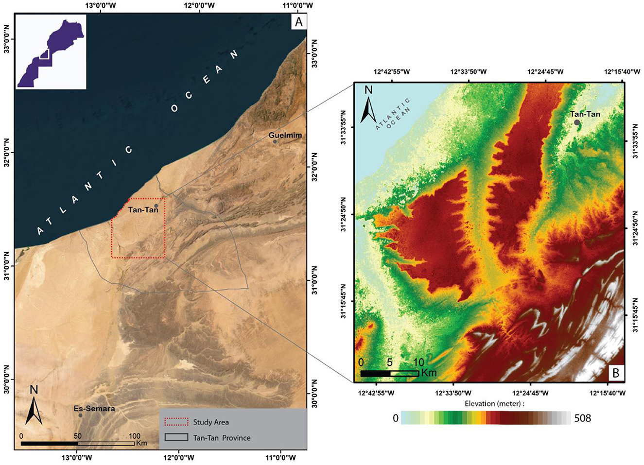
Figure 1. Location of study area within Tan-Tan province; (A) regional geographic location, (B) digital elevation map of study area.
Study area pedology is characterized by the abundance of eolian erosion soils. They are classified as poor quality soils with a high salt content; consequently, the agricultural production potential of these soils is very week. Well as, these soils present the absence of forest cover. Besides, the hydrographic network in the study area is characterized by seasonal and inter-annual irregularity of the inflows. The flow regime of the latter is considered as torrential and rapid. In order to limit the risks of flooding and contribute to the artificial recharge of the surface alluvial aquifers, the Moroccan government has built more than ten hill dams on several rivers. However, the majority of these rivers are not perennial and dry up for most of the year due to the arid climate of the province.
2.1 Geological setting of Tan-Tan area
The used geological map in this study (Figure 2) was derived from the Tan-Tan geological map (Scale of 1: 250, 000) provided by the Ministry of Energy Transition and Sustainable Development of Morocco, published last year. From a geological point of view, the study area is part of the Saharan coastal plateau located in south-west Morocco. The latter is located on the Atlantic coast, dipping westwards. The study area is formed of lithounits from Cambrian to Quaternary, which cover as well as show the outcropping of Neoproterozoic formations extended from the western Anti-Atlas (Choubert, 1963). Figure 2 shows also two cross-sections demonstrating the dominance of cretaceous formations in Tan-Tan region, which appears in the coastal domain.
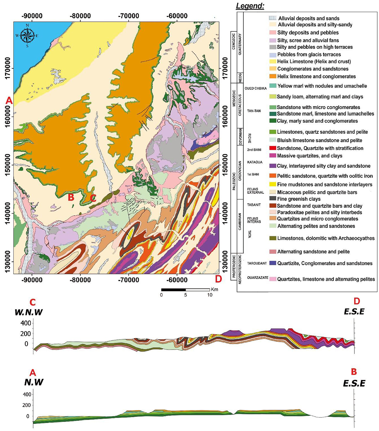
Figure 2. Geological map of Tan-Tan region and cross-sections.
Proterozoic lithounits are mainly formed by the quartzites from Neoproterozoic, which is ended by Adoudou formations. In general, the Precambrian and Triassic terrains are impermeable formations that have been discovered at depths of over 4,000 meters by drilling activities in the area. These formations form the bedrock of strategic aquifers located at considerable depths; the Cambrian is essentially formed by sandstone and pelite intercalations; the Ordovician shows in its bottom pelitique sandstone intercalations and mudstone, then topped by sandstone; Devonian period is essentially calcareous, formed by Riches formations (see Figure 2). Rich 1 showing Bluish Orthoceras limestone, quartzose sandstones, and interbedded pelitique layers, then, Rich 2 showing Crystalline lumachelles limestone, quartzose sandstones, and interbedded pelitique layers; the Lower Cretaceous strata are made up of two distinct lithological series: The first series corresponds to the continental Cretaceous, characterized by the presence of conglomerates, sands, sandstones, red clays and gypsum. These deposits have been identified at Oued Chebika by oil drilling. The second series corresponds to the marine Cretaceous, whose formations are widely exposed in the Hameidia, Telia and El Gueblia slopes. The lithology of this last series is mainly made up of detrital sedimentary rocks, in particular marly limestones which sometimes alternate with sandy marls. There are also coarse sediments such as sandstone and sand, which follow one another in the sequence. Both rock series have medium to high permeability, although they may contain significant groundwater reservoirs; the Neogene consists mainly of very impermeable limestone crusts. It outcrops in the Hamaidias hills. The coastal zone to the north of Tan-Tan is covered by a conglomeratic formation of Moghrebian age (Plio-Villafranchian), surmounted by permeable Quaternary formations comprising alluvial deposits, scree, alluvial fans and highly permeable limestone crusts. Recent alluvial deposits, which fill watercourses, are commonly considered to be alluvial aquifers, provided they are underlain by impermeable substrates and are of significant thickness. It is important to note that these two stratigraphic series constitute the different levels of surface aquifers in the study area (Bentayeb and Leclerc, 1977).
3 Materials and methods
Groundwater potential mapping is intrinsically dependent on a complex set of conditioning factors. In this study, a total of thirteen controlling groundwater-related factors are selected and grouped into four distinct categories: topographical, hydrological, geological and climatological factors. To assess the groundwater potential in this study area, the methodology summarized in the Figure 3 is adopted.
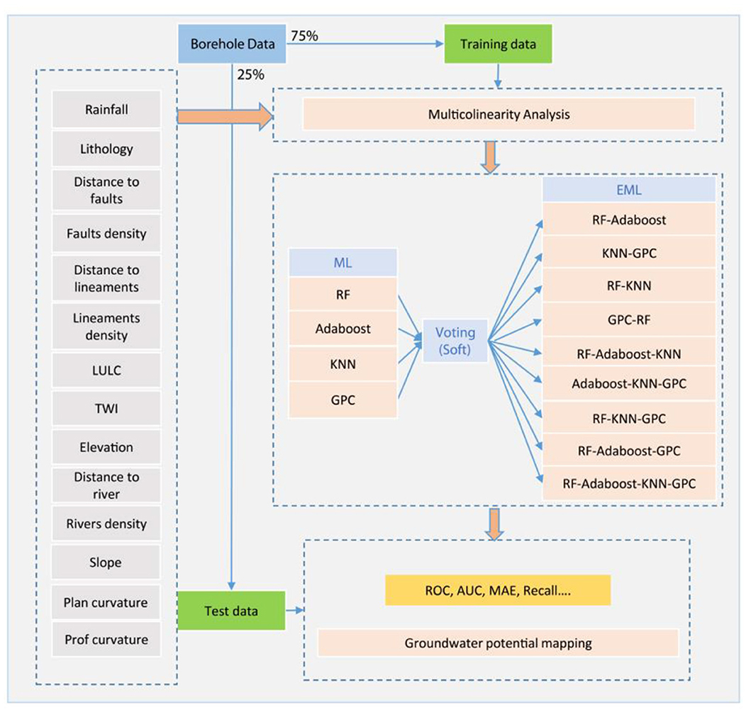
Figure 3. Flowchart applying single machine learning and ensemble learning techniques in groundwater potential mapping in the study area.
This analysis begins with (i) the preparation of data for modeling. This stage includes the setting up of layers representing the influencing factors and a layer listing the boreholes present in the study area. Then, in order to effectively select the factors contributing to the occurrence of groundwater (Multicolinearity), a technique based on the calculation of the variance inflation factor (VIF) was applied; (ii) The RF, Adaboost, KNN and GPC models were used to model groundwater potential; different sets of models were then tested to find the best prediction in the generated GWP maps; (iii) Several statistical parameters were applied to assess the precision of the results of applying the models, and an overall comparison was made on the basis of assessing the accuracy of the models.
3.1 Materials
3.1.1 Groundwater data
Over the last few decades, the province of Tan-Tan has been the scene of intense hydrogeological prospecting activity. A considerable amount of drilling works with a total of about 70,000 meters have been carried out, resulting in 1,500 groundwater potential sites. In this study, data relating to groundwater collection points and boreholes were collected from the Sakia El Hamra-Oued Eddahab hydraulic Basin Agency (AHB SHOE), Tan-Tan Provincial Directorate of Agriculture (DPA Tan-Tan) and [the National Agency for Drinking Water (ONEP)]. The groundwater potential was determined by analyzing the results of pumping tests carried out during the development phase of each water point by the organizations mentioned above. Consequently, boreholes with a flow rate >10.0 m3/s have been categorized as having a high potential for groundwater resources. In this context, more than 174 groundwater potential sites have been identified as having high potential. On the other hand, 133 water points are considered to be non-potential or to have limited potential in terms of groundwater supply (Figure 4). Due to the low frequency of non-productive or very low-yielding boreholes in the study area, we have included sampling data from areas where no groundwater abstraction has been carried out, in order to balance the input data set (Manna et al., 2022). The selection of non-potential sampling sites was based on in-depth geological and geophysical studies carried out as part of the groundwater prospecting programs. Boreholes considered to be productive were assigned a value of 1, indicating a high potential for water supply. On the other hand, low-yield boreholes, listed dry boreholes and sampling sites with non-groundwater potential were assigned a value of 0, indicating very limited groundwater potential.
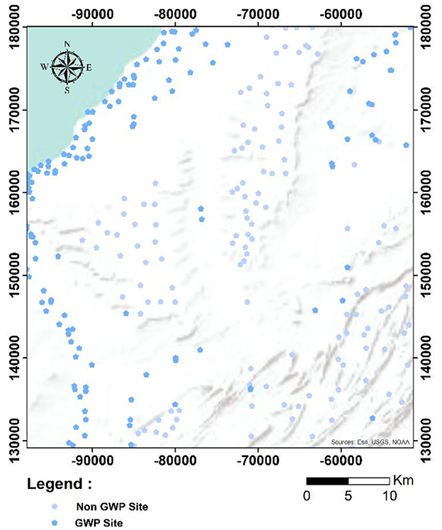
Figure 4. Groundwater potential and non-potential point's location. GWP, groundwater potential.
3.1.2 Conditioning factors
3.1.2.1 Hydrological factor
In order to assess surface water run-off and determine groundwater infiltration, it is necessary to take into account various hydrological factors, including drainage density and distance from the watercourse. The drainage process is controlled by hydrogeomorphological parameters such as geological composition, bedrock structure, soil permeability, type of vegetation cover and land topography (Razandi et al., 2015). Drainage density is quantified by the ratio between the total length of watercourses and the unit area of the study zone (Magesh et al., 2012).
3.1.2.2 Climatic factor
Precipitation is the main source of freshwater supply, which can either infiltrate aquifers or flow through watercourses. This depends on the specific topographical features of each region. This precipitation plays a fundamental role in the aquifer recharge process (Maity and Mandal, 2019). Various previous studies have revealed a positive correlation between precipitation levels and groundwater potential (Adiat et al., 2012). In this study, annual precipitation mapping was carried out using a time series of annual precipitation estimates from 2004 to 2014 in the Geotiff format of the PERSIANN-CSSCDR (Precipitation Estimation from Remotely Sensed Information Using Artificial Neural Networks—Climate Data) product and data measured at 20 existing weather stations around the study area. Next, annual precipitation was estimated using a polynomial model that was applied to satellite precipitation data (CCS-CDR PERSIANN). The data was then specialized using the raster calculator algorithm integrated into the ArcGIS 10.5 software. According to the rainfall map produced, average annual rainfall varies between 73 and 104 mm/year in the study area. The highest values are found in the northern part, while in the south precipitation decreases intensely (Figure 5A).

Figure 5. Used environmental factors for GWP modeling, (A) precipitation, (B) distance to faults, (C) fault density, (D) distance to lineaments, (E) lineament density, (F) land use/land cover, (G) TWI, (H) elevation, (I) distance to rivers, (J) rivers density, (K) slope, (L) plan curvature, (M) profile curvature and (N) lithology (refer to the geological map in Figure 2 for the abbreviations).
3.1.2.3 Geological factor
Lithology plays a crucial role in the permeability of aquifers (Jari et al., 2022) and geological faults increase the infiltration of rainwater due to the presence of highly permeable weathered materials. Faults can act as productive underground reservoirs by inducing the formation of an alteration zone around them (Jari et al., 2022). Accurate mapping of faults and surrounding areas is essential to identify potentially productive regions and discover new reservoirs in fractured zones (Jari et al., 2022). Lineaments are linear or curvilinear geological structures associated with various geomorphological or tectonic features (Adiri et al., 2017; Hajaj et al., 2022). Their orientation, density, and connectivity are important factors in their characterization (Hajaj et al., 2022). Lineament density is used as a hydrodynamic indicator to assess groundwater resources and identify productive zones (Razandi et al., 2015). The proximity of lineaments is also important for identifying hydrogeological zones of interest, generally near geological faults. In this study, the lithology and faults were mapped using the Tan-Tan geological map at a scale of 1:125,000. The maps were digitized in ArcGIS 10.5 software, where the fault density and Euclidean distance from the faults were calculated. The lineaments were mapped by filtering Landsat 8 OLI satellite images, and their accuracy was checked by comparing them with the fault maps from the Tan-Tan geological map.
3.1.2.4 Topographic factor
Topographic factors play a key role in regulating hydrological conditions, including groundwater flow and soil moisture. In this study, we used five topographic factors, namely elevation, slope, curvature, profile curvature, and plane curvature, as well as the topographic moisture index (TWI). These topographic factors were obtained from a digital terrain model and processed using the ArcGIS 10.5 environment, as illustrated in Figure 5. The topographic moisture index (TWI) is a parameter widely used to describe spatial moisture patterns and to explain the impact of topographic conditions on these patterns (Moore et al., 1991). The TWI influences the movement and accumulation of flows. When the TWI was calculated for the study area, it revealed the influence of topography on flow generation and flow accumulation. In general, high TWI values favor increased groundwater potential. Elevation and slope factors generally have a negative impact on groundwater potential, since in flat, low-lying areas rainwater has more time to infiltrate and recharge groundwater reserves (Jari et al., 2022).
3.1.2.5 LULC factor
Hydrological processes are strongly influenced by land use/cover factors (LULC), thereby exerting a significant impact on groundwater potentiality. Within the scope of this study, the study land cover map was performed: land use/land cover (LU/LC) layer was generated using supervised classification and the maximum likelihood algorithm in the ENVI software, based on the Sentinel-2A data. Concurrently, the resulting LULC map exhibited three distinct classes, including Water body, Built-up, Bare soil, Vegetation, Agriculture, and Forest (Figure 5). Table 1 shows the data sources used to generate the layers associated with each GW controlling Factor.
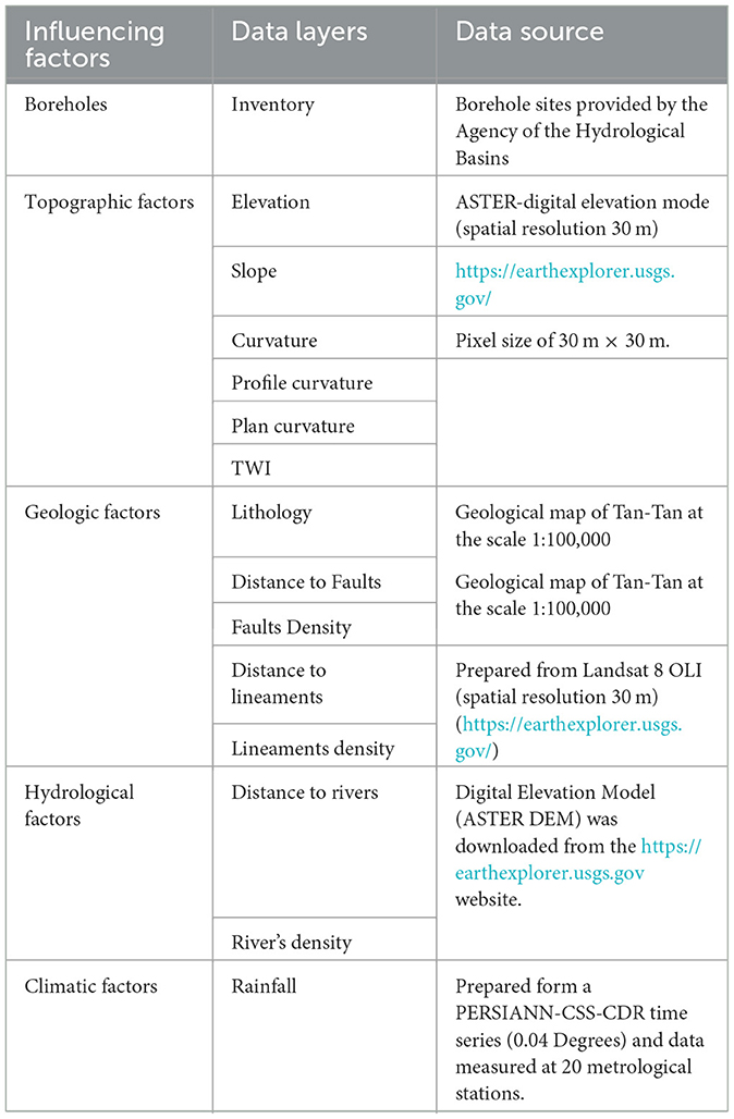
Table 1. Spatial database of the study area.
3.2 Methods
3.2.1 Random forest
The random forest (RF) (Breiman, 2001) is an ensemble classifier consisting of various individual decision trees which operate as an ensemble. Within the Random Forest, these individual trees partition class predictions, and the class with the highest number of votes is adopted as the model's prediction. This randomization helps to overfitting reduction and improves the generalization capabilities of the model. The final prediction of the Random Forest is achieved by aggregating the predictions of all the individual trees. This ensemble approach allows Random Forest to handle complex relationships and interactions between variables (see Supplementary Figure S1).
The description of the RF algorithm with a training dataset “d” and “n” features can be described as follows:
1. Use the bagging algorithm to create k random subsets (d1; d2; …; dk) from the training dataset d.
2. For each training subset dk, a decision tree model is created.
3. Combine the k trees h1(x1); h2 (x2); …; dk (xk) into a random forest ensemble, and determine the final classification results by aggregating majority votes from the individual trees.
In the training process, tuning hyperparameters for RF algorithm include n_estimators: number of trees in the forest; Criterion: in a decision tree, criterion dictates the method for measuring the split quality. Criterion, on the other hand, offers options as “entropy” for information gain or “gini” for Gini Impurity; Bootstrap: method for sampling data points is used in trees building. If “bootstrap” is set to “false”, the entire dataset is utilized for building each tree.
3.2.2 AdaBoost
The AdaBoost algorithm, known as Adaptive Boosting, was proposed by Freund and Schapire (1996). It has gained significant popularity as an iterative boosting algorithm for enhancing the performance of decision tree methods. AdaBoost effectively addresses the limitations of weak learners by iteratively correcting their errors and bolstering their abilities. The approach employed by AdaBoost involves sequentially adding weak learners to a model. These weak learners are trained on a training dataset that is weighted based on their performance. By incorporating this iterative procedure, AdaBoost transforms these initially weak models into strong ones. To create a robust final model, multiple weak learners are combined using a weighted voting scheme. The weights assigned to each weak learner reflect their individual contributions to the overall model's accuracy. In this manner, the final output model generated by AdaBoost benefits from the collective wisdom of the diverse weak learners. To formally depict The AdaBoost algorithm (Supplementary Figure S2), consider a training set denoted as dn = (x1, y1), …, (xn, yn). The algorithm proceeds for k iterations. During each iteration, for t = 1, …, k we select a base classifier h(k) from a set H of classifiers and assign it a coefficient α(k). In the basic version of the algorithm, H represents a finite collection of binary classifiers of the form h:ℝd → (−1, 1), and the base learner performs a comprehensive search within H during each iteration. The work of Freund and Schapire (1997) further emphasizes the effectiveness of AdaBoost, solidifying its standing as a powerful ensemble learning technique. In training process, adjustable hyperparameters include “n_estimators” for the quantity of weak learners trained iteratively and “learning_rate” that controlling each classifier's contribution. Balancing “learning_rate” with “n_estimators” significantly influences the model's performance and learning behavior.
3.2.3 K-nearest neighbor
The KNN algorithm is a non-parametric method. It is based on the principle that similar data points tend to have similar class labels or output values. For a given data set, the algorithm identifies its K nearest neighbors from the training dataset (Fix and Hodges, 1952; Cover and Hart, 1967) (see Supplementary Figure S3). The proximity between data points is typically determined using a distance metric, such as Euclidean distance or Manhattan distance. The K nearest neighbors are the K data points in the training set that have the smallest distances to the new data point. For classification, KNN employs a majority voting scheme among the K nearest neighbors to assign the class label to the new data point. The class label that occurs most frequently among the neighbors is considered the predicted class for the new data point. The K parameter in KNN determines the number of neighbors to consider. It is a crucial hyperparameter that needs to be carefully chosen. A smaller K value makes the model more sensitive to local variations, potentially leading to overfitting. Conversely, a larger K value can smooth out predictions but may lose local details.
3.2.4 Gaussian Process classification
Gaussian Process is probabilistic model used for regression and classification tasks. It is based on the concept of modeling functions as random variables, where any finite set of function values follows a joint Gaussian distribution (Hensman et al., 2015). Gaussian Process defines a distribution over functions, where each function is represented by its mean and covariance. The mean function provides the average behavior of the process, while the covariance function captures the relationships between different points in the input space. The choice of covariance function, also known as a kernel function, determines the smoothness, periodicity, and other properties of the functions generated by the GPC. The GP is determined by the mean function m(x) and the covariance function k(x, x′); f(x)~gp(m(x), k(x, x′)). GPC often referred to as a normal random process, represents a mathematical model that quantitatively characterizes the evolving connections among a sequence of stochastic events. GP relies on the utilization of the kernel function, which plays an important role in predictive and classification tasks by incorporating the hypothesis of the function to be acquired. In the training task, the hyperparameters configuration for the GPC model must be performed. The primary hyperparameter, crucially managed through the “kernel” argument, dictates the covariance function in Gaussian Processes (GP). Examples of frequently used kernels include RBF, WhiteKernel, Matern, DotProduct, and RationalQuadratic.
3.2.5 Ensemble machine learning
Ensemble learning is a method that involves training multiple machine learning models to produce enhanced predictions (Supplementary Figure S4), thereby boosting the performance compared to individual models. The term “ensemble” pertains to these predictors trained to collectively improve overall performance and predictive accuracy (Sagi and Rokach, 2018). Ensemble models work on the principle of the “wisdom of the crowd,” where diverse models contribute their unique perspectives, and their combined predictions often outperform any individual model. The underlying idea is that different models may have different strengths and weaknesses, and by combining their predictions, we can reduce biases and errors. Ensemble methods can be implemented by different types, including bagging, boosting, and stacking. Bagging is the approach used in the current research, multiple prediction models are trained on various subsets of the training dataset following bootstrapping. Then, the outputs of these models are combined using voting soft (for classification) in the final prediction. Bagging works well when the models used are diverse in nature and prone to overfitting. The choice of the ensemble in this study was based on a weighted aggregation of the individual RF, AB, GB and KNN models to determine the best possible combination. Three different combinations were tested: two models, three models and four models.
3.2.6 Grid search
A hyperparameter is a unique characteristic of a model whose value cannot be inferred from the data itself. In the context of any machine learning algorithm, the hyperparameter values must be established before the training process starts. This process serves as a means to identify the most suitable hyperparameter settings for a model, which, in turn, contributes to achieving higher prediction accuracy. Hyperparameter tuning can be perform through various methods, including grid search, random search, and manual exploration/n (Bergstra and Bengio, 2012). Grid search is a methodical approach for identifying the optimal hyperparameter configuration by automatically training models using all conceivable settings, as predefined within specified ranges of hyperparameter values. In this research, we integrated grid search into our program. Grid search has been applied to all machine learning models used in the current study.
3.2.7 Accuracy assessment
Results validation is a necessary stage to check the results performance as well as the results strength. On the other hand, by varying the dataset partitions, it is essential to evaluate the computation stability. In the order to perform this task, we have examined the following sample divisions: 55/45%, 65/35% and 75/25%. Thereafter, to assess the effectiveness of various ensemble methods, we applied statistical measures and calculated the area under the receiver operating characteristic curve (AUC) on the testing dataset.
The comparison between models is based on the calculation of the error criteria, FP-Rate, Kappa, MCC, RMSE, MSE, Sensitivity, Specificity, Accuracy and Precision. Higher values of Sensitivity, Specificity, Accuracy, Precision, FP-Rate, and MCC; lower values of RMSE and MSE; indicate a better performance of a model. A Kappa index value of 1 indicates a perfect model, whereas 0 represents a non-reliable model. The equations of the error criteria are written below (Equations 1–11):
Where,
TP True positive, TN True negative, FP False positive, FN False negative, n total number of predicted and real values, xp is the predicted classes, xa is the actual class.
To examine the excellence and the performance of machine learning models, the ROC curve represents a useful way to validate the results. The curve is a graphical representation that plots the true positive percentage in the y-axis and the cumulative false positive percentage in the x-axis. Finally, the area under the curve was calculated (AUC) from the ROC curve. The area under the ROC curve varies between 0 and 1; it can be categorized as low (0.5–0.6), medium (0.6–0.7), good (0.7–0.8), very good (0.8–0.9), and excellent (0.9–1.0) (Fawcett, 2006).
Where TP is the true positive, TN is the true negative, FP is the false positive, FN is the false negative, P is positive, and N is negative.
4 Results
4.1 Factors evaluation
GIF Screening and Analysis Following the initial stage of the analysis, which involved creating an inventory map of springs and non-springs as the foundational reference for the modeling phase, a thorough examination of the influential factors was conducted. This examination aimed to identify and retain the most relevant GIFs while eliminating those that exhibit no discernible impact or demonstrate multicollinearity. Multicollinearity analysis results show that VIF values of fifteen factors were all < 10, ranging from 1.044 to 8.162. However, the exact VIF (Variance Inflation Factor) threshold remains a topic of debate, consensus exists regarding a maximum threshold. If the VIF value of a factor surpasses 10.0 (or the tolerance drops below 0.1), it indicates a higher level of multicollinearity, which can potentially diminish the predictive capability the models (Kutner et al., 2004). The correlation matrix (CM) (Figure 6) depicted a strong positive correlation between elevation with line density (0.70), a moderate positive correlation between elevation and slope (0.40), line density and slope (0.51), distance to faults and distance to lines (0.49). A strong negative correlation was observed between rivers density and distance to river (−0.72). Indeed, there is no precise threshold as to what constitutes an acceptable level of correlation between two variables, although the literature shows that values between 0.4 and 0.85 can be acceptable (Dormann et al., 2013). However, the multicollinearity analysis demonstrates no required elimination of any factor, following their acceptable values in both of the VIF and CM (Table 2; Figure 6).

Figure 6. Correlation matrix of the fourteen GIFs for Multicolinearity analysis.

Table 2. Multicolinearity diagnosis for the groundwater influencing factors using the variance inflation factor (VIF).
4.2 GWPM
The primary aim of this investigation was to generate groundwater potential maps (GPMs) utilizing distinct and ensemble learning models. A total of thirteen model output combinations were generated by employing four models individually (RF, Adaboost, GPC, and KNN) as well as in ensemble configurations. Table 3 displays the hyperparameters employed in our models. The obtained GWPMs were subsequently categorized into five distinct classes using the Jenks' natural break classification method based on the calibration results. These classes were designated as very low, low, moderate, high, and very high. For the individual models, four groundwater potential maps are presented in Figure 7, where the GWPMs of RF, AdaBoost, KNN, and GPC were represented in Figures 7A–D, respectively. The integration of two or three models concurrently led to the development of novel GPM models, namely RF-AdaBoost (e), KNN-GPC, RF-GPC, AdaBoost-GPC, RF-AdaBoost-KNN, RF-KNN-GPC, Adaboost-KNN-GPC, and RF-AdaBoost-GPC. Figures 8E–L presents both the outcomes and spatial distribution of the distinct potentiality classes. Last, a set of the four models was used to produce another GPM model, RF-AdaBoost-KNN-GPC as shown in Figure 7M. Overall the models show that the very high GWP values are concentrated at the coastal part, and they are moderately represented in high river density zones. Meanwhile, the very low GWP values are localized in the central part within Neogene calcareous formations and the southwestern part of study area.

Table 3. Summary of the used hyperparameters.
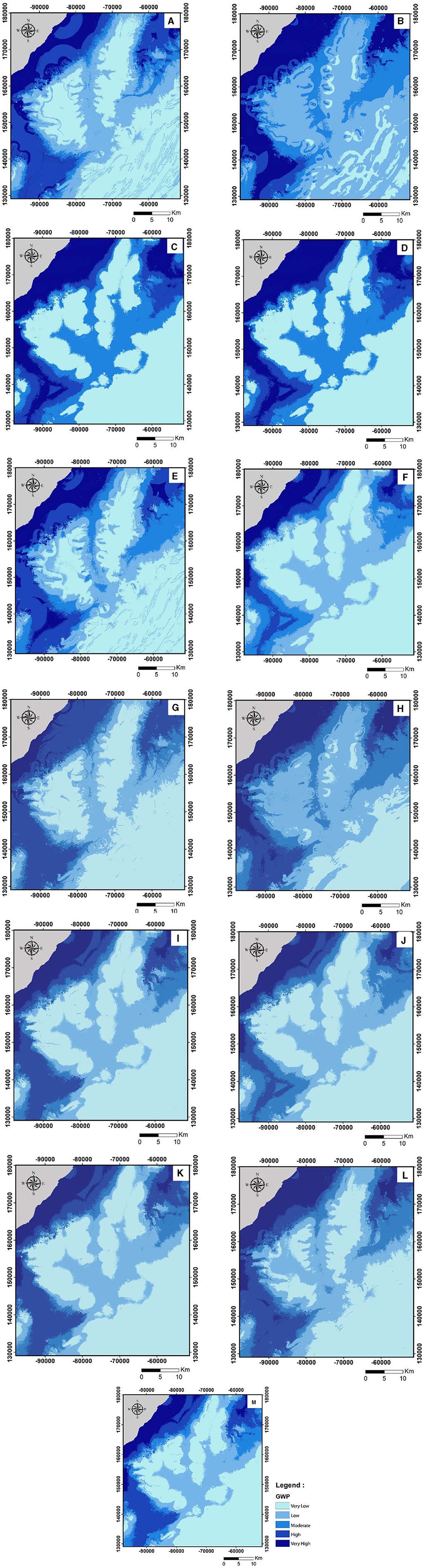
Figure 7. GWPM extracted using RF (A), AdaBoost (B), KNN (C), GPC (D), RF-AdaBoost (E), KNN-GPC (F), RF-GPC (G), AdaBoost-GPC (H), RF-AdaBoost-KNN (I), RF-KNN-GPC (J), Adaboost-KNN-GPC (K), RF-AdaBoost-GPC (L), and RF-AdaBoost-KNN-GPC (M).
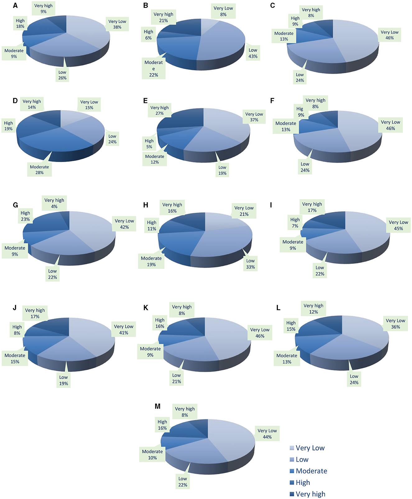
Figure 8. Percentage of the area occupied by GWP classes for the used models, RF (A), AdaBoost (B), KNN (C), GPC (D), RF-AdaBoost (E), KNN-GPC (F), RF-GPC (G), AdaBoost-GPC (H), RF-AdaBoost-KNN (I), RF-KNN-GPC (J), Adaboost-KNN-GPC (K), RF-AdaBoost-GPC (L), and RF-AdaBoost-KNN-GPC (M).
For the individual models (Figures 8A–D), the largest areas with very high GWP in a decreasing order were obtained by AdaBoost (21%), Gaussian process (14%), Random forest (9%), and K-nearest neighbor (8%). Besides the largest very low GWP areas in decreasing order were obtained by KNN (48%), Adaboost (43%), RF (38%), and Gaussian process (15%). Considering EM of two or three models (Figures 8E–L), the largest area with very high GWP was derived from RF-AdaBoost (27%) while the smallest was derived from RF-GPC (4%). On the other hand, the largest very low GWP area was derived from KNN-GPC and Adaboost-KNN-GPC (k) with (46%) while the smallest was obtained by h (21%). Concerning, the EM RF-AdaBoost-KNN-GPC (Figure 8M), the results show that the very low, low, moderate, high, and very high GWP covers 44, 22, 10, 16, and 8% of the study area, respectively. The EM with four models show a considerable similarity with RF and KNN, where much close values of GWP area percentages were revealed by the three models (Figure 8).
The determination of the success rate was based on the training dataset, providing an assessment of the model's accuracy in fitting the observed Groundwater Potential (GWP). Conversely, the prediction rate was evaluated using testing data, offering insights into the model's predictive performance for the GWP. To analyze the performance of the applied models, success and prediction rates were investigated across three different training/testing partitions: 55/45%, 65/35%, and 75/25% of the dataset. The corresponding results can be seen in Figure 9. The higher success rate was obtained by RF, FR-Adaboost, RF-GPC, and RF-Adaboost-KNN for the 75/25% partition. However, Adaboost and Adaboost-KNN-GPC displayed high prediction rates (0.95), while the ensemble models RF-GPC and RF-KNN-GPC showed the lowest prediction rate (0.92) for the 75/25% partition.
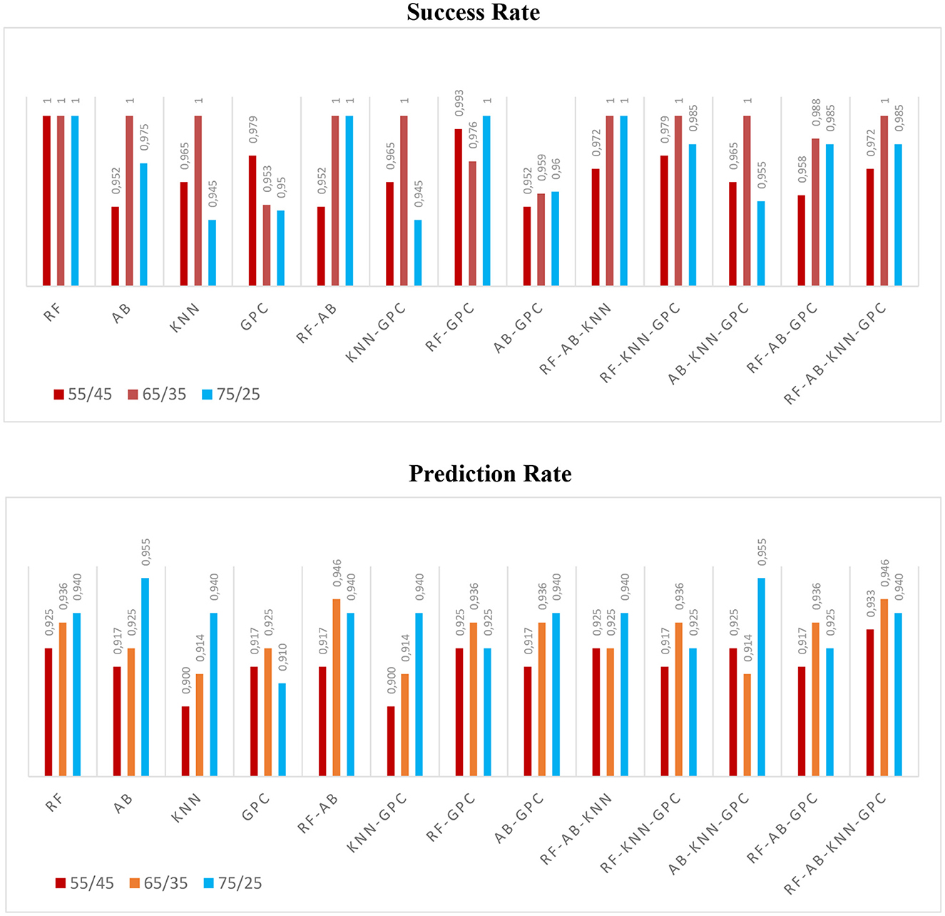
Figure 9. The success and prediction rates of the used ML and ensemble learning utilized models using 55/45%, 65/35%, and 75/25% partition.
In order to comprehensively evaluate the predictive performance of the thirteen models in terms of Groundwater Potential (GWP), various evaluation metrics including MSE, RMSE, R-square, F1-score, Specificity, kappa, MCC, Sensitivity, Pre, FFR, Ac, and AUC were assessed using both the training dataset (75%) and the testing dataset (25%). Moreover, the assessment of prediction capability for the thirteen models was accomplished through the examination of congruence between the training and validation inventories and the Groundwater Potential Maps (GPMs). Computed metrics for train and test were gathered in Table 4, respectively. For the training dataset, the RF, RF-AdaBoost, RF-GPC and RF-AdaBoost-KNN show an excellent prediction performance, presented by null MSE, RMSE and FPR (value = 0), and a maximum (value = 1) R square, F1-score, Spe, kappa, MCC, Sen, Pre, Ac, and AUC. The EMs RF-KNN-GPC, RF-AdaBoost-GPC, and RF-AdaBoost-KNN-GPC yield a good performance results following the minor gaps values with MSE = 0.015, RMSE = 0.12, an FPR = 0.01.
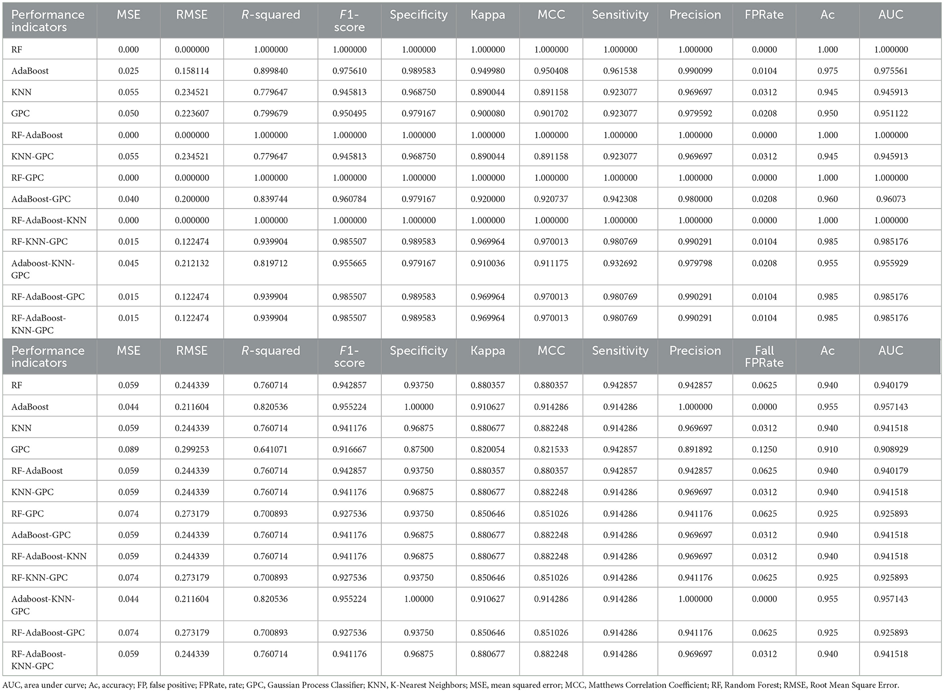
Table 4. Results of validation techniques based on training data and results of validation techniques based on test data.
Regarding the test dataset, various performance metrics were assessed. Assessing reliability through the MSE and RMSE methods, Adaboost and Adaboost-KNN-GPC models displayed the minimum values (MSE = 0.044, and RMSE = 0.21), whereas the GPC model exhibits the maximum values (MSE = 0.089, and RMSE = 0.30). R-squared presents a values range from 0.70 (RF-GPC, and RF-AdaBoost-GPC) and 0.76 that was achieved with several models including, RF, KNN, RF-Adaboost, and RF-AdaBoost-KNN-GPC. The computed F1-score ranges from 0.921 (GPC) and 0.9 (Adaboost and Adaboost-KNN-GPC). Accordingly, the accuracy values range from 0.91 to 0.95. Similar trends were observed for sensitivity, that has a maximum value of 0.94 (GPC and RF-Adaboost), while a minimum value of 0.14 observed in several models. Specificity varied between 0.93 (RF, RF-Adaboost, RF-GPC and RF-KNN-GPC) and 1.000 (Adaboost and Adaboost-KNN-GPC). Precision values ranged from 0.89 (GPC) and 1 (Adaboost and Adaboost-KNN-GPC).
In order to assess the prediction capability of the thirteen models, an evaluation was conducted by comparing the train and validation datasets with the GWPMs. The resulting rate curves, known as ROC curves, were generated, and the areas under each curve (AUCs) were computed (see Figure 10). The Area Under Curve (AUC) is a valuable metric that quantifies the system's ability to predict the presence or absence of “groundwater,” highlighting the significance of its estimation. Ranging from 0 to 1, AUC values provide insights into the predictive usefulness and accuracy of the models. Smaller AUC values indicate more meaningful predictions, while larger values indicate more precise estimations. The analysis of the train data (Figure 10 upper curves) revealed that the RF, RF-Adaboost, RF-GPC and RF-Adaboost-KNN models achieved the highest AUC value of 1.000, followed by RF-KNN-GPC, RF-Adaboost-GPC, RF-Adaboost-KNN-GPC and GPC with AUCs values superior to 0.97. Additionally, when comparing the validation data (Figure 10 lower curves) with GWPMs, it was observed that all models exhibited satisfactory performance for groundwater potentiality mapping, surpassing an AUC threshold of 0.90. Notably, Adaboost and Adaboost-KNN-GPC demonstrated the highest performance, with an AUC of 0.95. Almost all the models show an AUC of more than 0.94.

Figure 10. The area under curve (AUC) values for the models.
Figure 11 shows the prioritization rank of all the used models. Based on the analysis of Figure 11 the best success rates were revealed by RF, RF-Adaboost, RF-GPC, and RF-Adaboost-KNN models with (R-test = 1), while the EM models RF-KNN-GPC, RF-Adaboost-GPC, and FR-Adaboost-KNN-GPC show a considerable success rate (R-test = 5). Besides the best prediction rate was achieved by Adaboost, and Adaboost-KNN-GPC with R-train = 1, whereas a good prediction rate was observed with numerous models (R-train = 3) including, KNN, KNN-GPC, Adaboost-GPC, RF-Adaboost-KNN and FR-Adaboost-KNN-GPC. By considering both of success and prediction rate, prioritization analysis demonstrated that the best results were achieved by the EMs RF-Adaboost-KNN and FR-Adaboost-KNN-GPC demonstrating the benefit of ensemble modeling implementation in models stabilization (see Figure 11).
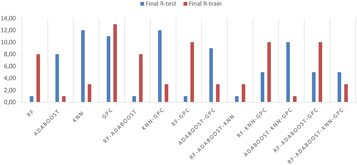
Figure 11. Prioritization graph extracted for the thirteen applied models.
Feature importance refers to the degree of influence or relevance of different features or variables on a model performance (Hooker et al., 2019). It is used to identify which features have the most impact on the model. The feature with a higher score means that the specific feature will have a larger effect on the model performance than others. Negative feature importance value means that the feature makes the loss go up. Feature importance allows us to understand the relationship between the features and the target variable, and also helps to understand what features are irrelevant for the model. As can be seen in Figure 12, variables TWI is identified as the important input for the RF model about 12%. For the KNN model, the variables of distance to faults, Slope, Rainfall, and LULC (respectively with the values of 10, 6.5, 6, and 3.5%) had a higher contribution in the modeling process. Additionally, for AdaBoost model, results have demonstrated that the variables of lines density, elevation, and LULC were the most important variables which had the values of 32, 6.5, 4%. For the GPC model, the variables fault density, LULC and Lithology had the most importance with the values of 6.2, 3.8, 2%.

Figure 12. Importance of the input variables for the used machine learning algorithms.
5 Discussion
The investigation described aims to generate groundwater potential maps (GPMs) using different machine learning models, both individually and in ensemble configurations. The study utilized four models: Random Forest (RF), Adaboost, Gaussian Process Classifier (GPC), and K-Nearest Neighbors (KNN). Thirteen model output combinations were generated, including individual models and ensemble models. The generated GPMs were categorized into five distinct classes: very low, low, moderate, high, and very high. These classes were determined using the Jenks' natural break classification method based on calibration results. Figures 7A–D presents the groundwater potential maps for the individual models (RF, Adaboost, KNN, and GPC), while Figures 7E–M shows the GPMs for the ensemble models. The distribution of groundwater potential classes is described based on the GPMs. The very high groundwater potential values are concentrated in the coastal part of the study area and moderately represented in high river density zones. Conversely, the very low groundwater potential values are localized in the central part within Neogene calcareous formations and the southwestern part of the study area.
The success and prediction rates of the models were analyzed to evaluate their performance. Three different training/testing partitions were used: 55/45%, 65/35%, and 75/25% of the dataset. The success rate represents the model's accuracy in fitting the observed groundwater potential, while the prediction rate indicates the model's predictive performance. Figure 9 displays the success and prediction rates for each model and partition. The performance indicators, including MSE, RMSE, R-squared, F1-score, specificity, Kappa, MCC, sensitivity, precision, fall FPRate, Accuracy and area AUC, were calculated for each model. Table 4 presents the results of the validation techniques based on training and test data. From the results, it can be observed that RF consistently achieved a high success rate (1) across all partitions. Adaboost and EN Adaboost-KNN-GPC demonstrated high prediction rates (0.95), while the ensemble models RF-GPC and RF-KNN-GPC had the lowest prediction rate (0.92) for the 75/25% partition. The AUC values, shown in Figure 10, provide further insights into the performance of the models.
The Random Forest model (RF) alone also performs well, achieving the lowest prioritization rank on the test data (R-test = 1.00). It demonstrates strong predictive capabilities and generalization power. The AdaBoost model performs exceptionally well on the train data (R-train = 1.00) but shows a slightly higher prioritization rank on the test data (R-test = 8.00), suggesting some degree of overfitting. Even, the inclusion of Adaboost with RF has no significant improvement in increasing the prioritization of RF in terms of prediction performance. The prediction rate rank of RF remain week (R-train =8.00) after applying the EM RF-Adaboost. Additionally, the inclusion of the K-Nearest Neighbors (KNN) in the two EM as RF-AdaBoost-KNN combination further enhances the model's stability. It achieves competitive results on both test and train data, indicating a good balance between generalizations and fitting the training data. This combination is likely to provide accurate predictions and maintain stability across various datasets, making it a reliable choice for practical applications. Although KNN alone has relatively a weak prioritization ranks on test data (R-test = 12.00), its incorporation into the ensemble contributes to a more robust prediction as well as permitted the optimization of RF prediction rate. The RF-AdaBoost-KNN ensemble model superior performance can be attributed to the strengths of its constituent models. RF excels in identifying complex patterns, and providing variable importance measures. RF when used individually demonstrated a good performance in GWP studies in other Moroccan areas, outperforming Linear regression (LR), decision trees (DT), and artificial neural networks (ANN) models in High Atlas Mountains (Namous et al., 2021). KNN captures local patterns and relationships in an unknown data distribution (Liu et al., 2019). Adaboost enhances accuracy by combining multiple weak learners and adjusting weights based on misclassified instances (Carty, 2011).
By leveraging the strengths of these models, the ensemble model achieves high performance in GWP mapping accuracy. Accordingly, numerous studies demonstrated the stability and the high prediction capability of ensemble learning, compared to individual ML algorithms (Tiwari and Chatterjee, 2010). It's important to note that model selection should also consider other factors such as computational efficiency, interpretability, and specific requirements of the problem. Additionally, it's recommended to further validate the performance of the chosen combination using cross-validation or additional evaluation metrics to ensure its effectiveness in real-world scenarios. Following a comprehensive analysis of factors influencing groundwater, our results align with previous research emphasizing the significant role of land use, lithology, and fault density in predicting groundwater spatial potentiality (Senanayake et al., 2016; Senthilkumar et al., 2019; Jaafarzadeh et al., 2021).
As limitation, the used of the totality of the factors that were reported in bibliography in the same area is a challenging task. The application of ML algorithms should be with caution in the order to avoid misclassifications and overfitting issues. However, in our study the evapotranspiration factor (i.e., evaporation) has been avoided. The non-integration of evaporation layer is explained by the geographical location of the studies area. Indeed, the proximity to the ocean often means that seawater intrusion can be a significant concern for groundwater resources. Additionally, the variable salinity of coastal groundwater systems can complicate the relationship between evaporation and groundwater. The coming studies by the authors will consider this thematic. In arid region, it has been empirically established that the evaporation factor exerts a pronounced influence on groundwater. This influence is particularly pronounced due to evaporation rates in these areas, which can exceed rainfall rates by several times or even by an order of magnitude, thereby significantly impacting groundwater reserves (Wang et al., 2022). On the other hand, the training dataset presents only 174 GWP sites. The amount of the used data can limit the application of DL models within the study area. However, the ML and EL algorithms show a satisfactory findings in terms of accuracy (see Table 4). Overall, the investigation utilized ensemble learning models to generate groundwater potential maps and evaluate their performance using various metrics. The results highlight the potential of these models for assessing groundwater potential and can provide valuable information for water resource management and planning.
6 Conclusion
This study employed a diverse range of methodologies in GIS environment, based on remote sensing, as well as individual and ensemble machine learning algorithms to assess Groundwater Potential (GWP) in extensive Saharan coastal water-scarce region. The unique characteristics of the study area, characterized by its coastal position and a low background in groundwater prospectivity as evidenced by low well points, posed distinct challenges in groundwater potential mapping (GWPM). These challenges led us to explore the utility of ensemble models for a more robust assessment. Multiple machine learning algorithms, including RF, AB, KNN, and GPC models, were employed for GWP mapping, chosen due to their satisfactory performance in other global regions. Individual model application revealed that RF exhibited the highest success rate, while not achieving a very high prediction rate. Besides the Adaboost model shows the inverse with a high prediction rate and a not showing a very high success rate. To further enhance prediction accuracy and robustness, ensemble models with two, three, and four algorithms have been applied. The RF-AB -KNN and RF-Adaboost-KNN-GPC were developed to explore their capacity to accurate prediction of groundwater potential zones in the study area, showing their high stability. The AUC (Area Under the Curve) metric showed notable improvement, with the ensemble model achieving the highest value of AUC = 0.94. Furthermore, various statistical metrics were applied to assess the efficiency and dependability of the various ensembles and individual models, culminating in a prioritization rank. The RF-AB-KNN ensemble model yielded the most promising results. This study's methodology holds potential for identifying groundwater potential zones, particularly in challenging-to-access mountainous regions, where implementing geophysical exploration methods remains costly and logistically demanding for vast areas. The outcomes of this study hold great importance for authorities and decision-makers for planning and managing groundwater resources, especially for urban and agricultural needs.
Data availability statement
The raw data supporting the conclusions of this article will be made available by the authors, without undue reservation.
Author contributions
AJa: Conceptualization, Data curation, Methodology, Software, Writing—original draft. EB: Project administration, Supervision, Validation, Writing—review & editing. SH: Methodology, Software, Validation, Visualization, Writing—original draft, Writing—review & editing. AK: Resources, Writing—review & editing. YK: Conceptualization, Methodology, Software, Writing—review & editing. AE: Methodology, Supervision, Validation, Writing—review & editing. AJe: Writing—original draft, Writing—review & editing. MN: Validation, Writing—review & editing.
Funding
The author(s) declare that no financial support was received for the research, authorship, and/or publication of this article.
Conflict of interest
The authors declare that the research was conducted in the absence of any commercial or financial relationships that could be construed as a potential conflict of interest.
Publisher's note
All claims expressed in this article are solely those of the authors and do not necessarily represent those of their affiliated organizations, or those of the publisher, the editors and the reviewers. Any product that may be evaluated in this article, or claim that may be made by its manufacturer, is not guaranteed or endorsed by the publisher.
Supplementary material
The Supplementary Material for this article can be found online at: https://www.frontiersin.org/articles/10.3389/frwa.2023.1305998/full#supplementary-material
References
Adiat, K., Nawawi, M., and Abdullah, K. (2012). Assessing the accuracy of GIS-based elementary multi criteria decision analysis as a spatial prediction tool–a case of predicting potential zones of sustainable groundwater resources. J. Hydrol. 440, 75–89. doi: 10.1016/j.jhydrol.2012.03.028
Adiri, Z., El Harti, A., Jellouli, A., Lhissou, R., Maacha, L., Azmi, M., et al. (2017). Comparison of Landsat-8, ASTER and Sentinel 1 satellite remote sensing data in automatic lineaments extraction: a case study of Sidi Flah-Bouskour inlier, Moroccan Anti Atlas. Adv. Space Res. 60, 2355–2367. doi: 10.1016/j.asr.2017.09.006
Ahmad, I., Hasan, H., Jilani, M. M., and Ahmed, S. I. (2023). Mapping potential groundwater accumulation zones for Karachi city using GIS and AHP techniques. Environ. Monit. Assess. 195, 381. doi: 10.1007/s10661-023-10971-x
Anh, D. T., Pandey, M., Mishra, V. N., Singh, K. K., Ahmadi, K., Janizadeh, S., et al. (2023). Assessment of groundwater potential modeling using support vector machine optimization based on Bayesian multi-objective hyperparameter algorithm. Appl. Soft Comput. 132, 109848. doi: 10.1016/j.asoc.2022.109848
Arabameri, A., Pal, S. C., Rezaie, F., Nalivan, O. A., Chowdhuri, I., Saha, A., et al. (2021). Modeling groundwater potential using novel GIS-based machine-learning ensemble techniques. J. Hydrol. 36, 100848. doi: 10.1016/j.ejrh.2021.100848
Bai, Z., Liu, Q., and Liu, Y. (2022). Groundwater potential mapping in hubei region of china using machine learning, ensemble learning, deep learning and automl methods. Nat. Resour. Res. 31, 2549–2569. doi: 10.1007/s11053-022-10100-4
Bentayeb, A., and Leclerc, C. (1977). Les ressources en eau du Maroc, tome 3, domaines atlasique et sud-atlasique. Service Geologique du Maroc, 37–84.
Bergstra, J., and Bengio, Y. (2012). Random search for hyper-parameter optimization. J. Mach. Learn. Res. 13.
Carty, D. M. (2011). An analysis of boosted regression trees to predict the strength properties of wood composites (Masters Theses). The University of Tennessee Knoxville, Knoxville, TN, United States.
Choubert, G. (1963). Essai de mise au point du problème des “ignimbrites”. Bull. Volcanol. 25, 123–140. doi: 10.1007/BF02596545
Cover, T., and Hart, P. (1967). Nearest neighbor pattern classification. IEEE Transact. Inf. Theory 13, 21–27. doi: 10.1109/TIT.1967.1053964
Dormann, C. F., Elith, J., Bacher, S., Buchmann, C., Carl, G., Carré, G., et al. (2013). Collinearity: a review of methods to deal with it and a simulation study evaluating their performance. Ecography 36, 27–46. doi: 10.1111/j.1600-0587.2012.07348.x
Elbeltagi, A., Kumar, N., Chandel, A., Arshad, A., Pande, C. B., and Islam, A. R. M. T. (2022). Modelling the reference crop evapotranspiration in the Beas-Sutlej basin (India): an artificial neural network approach based on different combinations of meteorological data. Environ. Monit. Assess. 194, 141. doi: 10.1007/s10661-022-09812-0
Fawcett, T. (2006). An introduction to ROC analysis. Pattern Recognit. Lett. 27, 861–874. doi: 10.1016/j.patrec.2005.10.010
Fix, E., and Hodges Jr, J. L. (1952). Discriminatory Analysis-Nonparametric Discrimination: Small Sample Performance. Berkeley, CA: California Univ.
Freund, Y., and Schapire, R. E. (1996). “Experiments with a new boosting algorithm,” in icml (Citeseer), 148–156.
Freund, Y., and Schapire, R. E. (1997). A decision-theoretic generalization of on-line learning and an application to boosting. J. Comp. Syst. Sci. 55, 119–139. doi: 10.1006/jcss.1997.1504
Garg, R., Kumar, A., Prateek, M., Pandey, K., and Kumar, S. (2022). Land cover classification of spaceborne multifrequency SAR and optical multispectral data using machine learning. Adv. Space Res. 69, 1726–1742. doi: 10.1016/j.asr.2021.06.028
Guo, X., Gui, X., Xiong, H., Hu, X., Li, Y., Cui, H., et al. (2023). Critical role of climate factors for groundwater potential mapping in arid regions: Insights from random forest, XGBoost, and LightGBM algorithms. J. Hydrol. 621, 129599. doi: 10.1016/j.jhydrol.2023.129599
Haggerty, R., Sun, J., Yu, H., and Li, Y. (2023). Application of machine learning in groundwater quality modeling-A comprehensive review. Water Res. 233, 119745. doi: 10.1016/j.watres.2023.119745
Hajaj, S., El Harti, A., and Jellouli, A. (2022). Assessment of hyperspectral, multispectral, radar, and digital elevation model data in structural lineaments mapping: A case study from Ameln valley shear zone, Western Anti-Atlas Morocco. Remote Sens. Appl. 27, 100819. doi: 10.1016/j.rsase.2022.100819
Hajaj, S., El Harti, A., Jellouli, A., Pour, A. B., Mnissar Himyari, S., Hamzaoui, A., et al. (2023). Evaluating the performance of machine learning and deep learning techniques to hymap imagery for lithological mapping in a semi-arid region: case study from Western Anti-Atlas, Morocco. Minerals 13, 766. doi: 10.3390/min13060766
Hakim, W. L., Nur, A. S., Rezaie, F., Panahi, M., Lee, C.-W., and Lee, S. (2022). Convolutional neural network and long short-term memory algorithms for groundwater potential mapping in Anseong, South Korea. J. Hydrol. 39, 100990. doi: 10.1016/j.ejrh.2022.100990
Hensman, J., Matthews, A., and Ghahramani, Z. (2015). “Scalable variational Gaussian process classification,” in Proceedings of the 18th International Conference on Artificial Intelligence and Statistics (AISTATS) (San Diego, CA: PMLR), 351–360.
Hooker, S., Erhan, D., Kindermans, P.-J., and Kim, B. (2019). A benchmark for interpretability methods in deep neural networks. Adv. Neural Inf. Process. Syst. 32.
Jaafarzadeh, M. S., Tahmasebipour, N., Haghizadeh, A., Pourghasemi, H. R., and Rouhani, H. (2021). Groundwater recharge potential zonation using an ensemble of machine learning and bivariate statistical models. Sci. Rep. 11, 5587. doi: 10.1038/s41598-021-85205-6
Jari, A., El Mostafa Bachaoui, A. J., El Harti, A., Khaddari, A., and El Jazouli, A. (2022). Use of GIS, remote sensing and analytical hierarchy process for groundwater potential assessment in an arid region–a case study. Ecol. Eng. 5, 234–255. doi: 10.12912/27197050/152141
Jari, A., Khaddari, A., Hajaj, S., Bachaoui, E. M., Mohammedi, S., Jellouli, A., et al. (2023). Landslide susceptibility mapping using multi-criteria decision-making (MCDM), statistical, and machine learning models in the Aube Department, France. Earth 4, 698–713. doi: 10.3390/earth4030037
Khan, J., Lee, E., Balobaid, A. S., and Kim, K. (2023). A Comprehensive review of conventional, machine leaning, and deep learning models for groundwater level (GWL) forecasting. Appli. Sci. 13, 2743. doi: 10.3390/app13042743
Kutner, M. H., Nachtsheim, C. J., Neter, J., and Wasserman, W. (2004). Applied Linear Regression Models. New York, NY: McGraw-Hill/Irwin.
Liu, Z.-G., Zhang, Z., Liu, Y., Dezert, J., and Pan, Q. (2019). A new pattern classification improvement method with local quality matrix based on K-NN. Knowl. Based Syst. 164, 336–347. doi: 10.1016/j.knosys.2018.11.001
Magesh, N. S., Chandrasekar, N., and Soundranayagam, J. P. (2012). Delineation of groundwater potential zones in Theni district, Tamil Nadu, using remote sensing, GIS and MIF techniques. Geosci. Front. 3, 189–196. doi: 10.1016/j.gsf.2011.10.007
Maity, D. K., and Mandal, S. (2019). Identification of groundwater potential zones of the Kumari river basin, India: an RS & GIS based semi-quantitative approach. Environ. Dev. Sustain. 21, 1013–1034. doi: 10.1007/s10668-017-0072-0
Manna, F., Kennel, J., and Parker, B. (2022). Understanding mechanisms of recharge through fractured sandstone using high-frequency water-level-response data. Hydrogeol. J. 30, 1599–1618. doi: 10.1007/s10040-022-02515-3
Masroor, M., Sajjad, H., Kumar, P., Saha, T. K., Rahaman, M. H., Choudhari, P., et al. (2023). Novel Ensemble machine learning modeling approach for groundwater potential mapping in Parbhani District of Maharashtra, India. Water 15, 419. doi: 10.3390/w15030419
Moore, I. D., Grayson, R., and Ladson, A. (1991). Digital terrain modelling: a review of hydrological, geomorphological, and biological applications. Hydrol. Process. 5, 3–30. doi: 10.1002/hyp.3360050103
Morgan, H., Madani, A., Hussien, H. M., and Nassar, T. (2023). Using an ensemble machine learning model to delineate groundwater potential zones in desert fringes of East Esna-Idfu area, Nile valley, Upper Egypt. Geosci. Lett. 10, 9. doi: 10.1186/s40562-023-00261-2
Mosavi, A., Sajedi Hosseini, F., Choubin, B., Goodarzi, M., Dineva, A. A., and Rafiei Sardooi, E. (2021). Ensemble boosting and bagging based machine learning models for groundwater potential prediction. Water Resour. Manag. 35, 23–37. doi: 10.1007/s11269-020-02704-3
Naghibi, S. A., Dolatkordestani, M., Rezaei, A., Amouzegari, P., Heravi, M. T., Kalantar, B., et al. (2019). Application of rotation forest with decision trees as base classifier and a novel ensemble model in spatial modeling of groundwater potential. Environ. Monit. Assess. 191, 1–20. doi: 10.1007/s10661-019-7362-y
Naghibi, S. A., Moghaddam, D. D., Kalantar, B., Pradhan, B., and Kisi, O. (2017). A comparative assessment of GIS-based data mining models and a novel ensemble model in groundwater well potential mapping. J. Hydrol. 548, 471–483. doi: 10.1016/j.jhydrol.2017.03.020
Namous, M., Hssaisoune, M., Pradhan, B., Lee, C.-W., Alamri, A., Elaloui, A., et al. (2021). Spatial prediction of groundwater potentiality in large semi-arid and karstic mountainous region using machine learning models. Water 13, 2273. doi: 10.3390/w13162273
Orimoloye, I. R., Olusola, A. O., Belle, J. A., Pande, C. B., and Ololade, O. O. (2022). Drought disaster monitoring and land use dynamics: identification of drought drivers using regression-based algorithms. Nat. Hazards 112, 1085–1106. doi: 10.1007/s11069-022-05219-9
Ouali, L., Kabiri, L., Namous, M., Hssaisoune, M., Abdelrahman, K., Fnais, M. S., et al. (2023). Spatial prediction of groundwater withdrawal potential using shallow, hybrid, and deep learning algorithms in the Toudgha Oasis, Southeast Morocco. Sustainability 15, 3874. doi: 10.3390/su15053874
Pham, B. T., Jaafari, A., Van Phong, T., Mafi-Gholami, D., Amiri, M., Van Tao, N., et al. (2021). Naïve Bayes ensemble models for groundwater potential mapping. Ecol. Inform. 64, 101389. doi: 10.1016/j.ecoinf.2021.101389
Rahmati, O., Pourghasemi, H. R., and Melesse, A. M. (2016). Application of GIS-based data driven random forest and maximum entropy models for groundwater potential mapping: a case study at Mehran Region, Iran. Catena 137, 360–372. doi: 10.1016/j.catena.2015.10.010
Razandi, Y., Pourghasemi, H. R., Neisani, N. S., and Rahmati, O. (2015). Application of analytical hierarchy process, frequency ratio, and certainty factor models for groundwater potential mapping using GIS. Earth Sci. Inf. 8, 867–883. doi: 10.1007/s12145-015-0220-8
Sachdeva, S., and Kumar, B. (2021). Comparison of gradient boosted decision trees and random forest for groundwater potential mapping in Dholpur (Rajasthan), India. Stochast. Environ. Res. Risk Assess. 35, 287–306. doi: 10.1007/s00477-020-01891-0
Sagi, O., and Rokach, L. (2018). Ensemble learning: a survey. Wiley Interdiscipl. Rev. 8, e1249. doi: 10.1002/widm.1249
Sangawi, A., Al-Manmi, D. A. M., and Aziz, B.Q. (2023). Integrated GIS, remote sensing, and electrical resistivity tomography methods for the delineation of groundwater potential zones in Sangaw Sub-Basin, Sulaymaniyah, KRG-Iraq. Water 15, 1055. doi: 10.3390/w15061055
Senanayake, I., Dissanayake, D., Mayadunna, B., and Weerasekera, W. (2016). An approach to delineate groundwater recharge potential sites in Ambalantota, Sri Lanka using GIS techniques. Geosci. Front. 7, 115–124. doi: 10.1016/j.gsf.2015.03.002
Senthilkumar, M., Gnanasundar, D., and Arumugam, R. (2019). Identifying groundwater recharge zones using remote sensing & GIS techniques in Amaravathi aquifer system, Tamil Nadu, South India. Sustain. Environ. Res. 29, 1–9. doi: 10.1186/s42834-019-0014-7
Shelar, R. S., Nandgude, S. B., Pande, C. B., Costache, R., El-Hiti, G. A., Tolche, A. D., et al. (2023). Unlocking the hidden potential: groundwater zone mapping using AHP, remote sensing and GIS techniques. Geomat. Nat. Hazards Risk 14, 2264458. doi: 10.1080/19475705.2023.2264458
Tamiru, H., and Wagari, M. (2022). Comparison of ANN model and GIS tools for delineation of groundwater potential zones, Fincha Catchment, Abay Basin, Ethiopia. Geocarto Int. 37, 6736–6754. doi: 10.1080/10106049.2021.1946171
Thanh, N. N., Thunyawatcharakul, P., Ngu, N. H., and Chotpantarat, S. (2022). Global review of groundwater potential models in the last decade: parameters, model techniques, and validation. J. Hydrol. 128501. doi: 10.1016/j.jhydrol.2022.128501
Tiwari, M. K., and Chatterjee, C. (2010). Development of an accurate and reliable hourly flood forecasting model using wavelet–bootstrap–ANN (WBANN) hybrid approach. J. Hydrol. 394, 458–470. doi: 10.1016/j.jhydrol.2010.10.001
Van Phong, T., and Pham, B. T. (2023). Performance of Naïve Bayes Tree with ensemble learner techniques for groundwater potential mapping. Phys. Chem. Earth Parts A/B/C 103503. doi: 10.1016/j.pce.2023.103503
Wang, Z., Wang, J., and Han, J. (2022). Spatial prediction of groundwater potential and driving factor analysis based on deep learning and geographical detector in an arid endorheic basin. Ecol. Indic. 142, 109256. doi: 10.1016/j.ecolind.2022.109256
Keywords: groundwater potential mapping, machine learning, ensemble learning, arid regions, Tan-Tan region, Morocco
Citation: Jari A, Bachaoui EM, Hajaj S, Khaddari A, Khandouch Y, El Harti A, Jellouli A and Namous M (2023) Investigating machine learning and ensemble learning models in groundwater potential mapping in arid region: case study from Tan-Tan water-scarce region, Morocco. Front. Water 5:1305998. doi: 10.3389/frwa.2023.1305998
Received: 02 October 2023; Accepted: 20 November 2023;
Published: 13 December 2023.
Edited by:
Francesco Granata, University of Cassino, ItalyReviewed by:
Fabio Di Nunno, University of Cassino, ItalyChaitanya B. Pande, Indian Institute of Tropical Meteorology (IITM), India
Copyright © 2023 Jari, Bachaoui, Hajaj, Khaddari, Khandouch, El Harti, Jellouli and Namous. This is an open-access article distributed under the terms of the Creative Commons Attribution License (CC BY). The use, distribution or reproduction in other forums is permitted, provided the original author(s) and the copyright owner(s) are credited and that the original publication in this journal is cited, in accordance with accepted academic practice. No use, distribution or reproduction is permitted which does not comply with these terms.
*Correspondence: Soufiane Hajaj, c291ZmlhbmVoYWphajEzQGdtYWlsLmNvbQ==; Abdessamad Jari, amFyaWdlb21pbmVzZnB0QGdtYWlsLmNvbQ==