1
NeuroMathComp Laboratory, INRIA/ENS, France
2
Laboratoire Jean-Alexandre Dieudonné, Nice, France
3
Université de Nice, Nice, France
We deal with the problem of bridging the gap between two scales in neuronal modeling. At the first (microscopic) scale, neurons are considered individually and their behavior described by stochastic differential equations that govern the time variations of their membrane potentials. They are coupled by synaptic connections acting on their resulting activity, a nonlinear function of their membrane potential. At the second (mesoscopic) scale, interacting populations of neurons are described individually by similar equations. The equations describing the dynamical and the stationary mean-field behaviors are considered as functional equations on a set of stochastic processes. Using this new point of view allows us to prove that these equations are well-posed on any finite time interval and to provide a constructive method for effectively computing their unique solution. This method is proved to converge to the unique solution and we characterize its complexity and convergence rate. We also provide partial results for the stationary problem on infinite time intervals. These results shed some new light on such neural mass models as the one of Jansen and Rit (1995)
: their dynamics appears as a coarse approximation of the much richer dynamics that emerges from our analysis. Our numerical experiments confirm that the framework we propose and the numerical methods we derive from it provide a new and powerful tool for the exploration of neural behaviors at different scales.
Modeling neural activity at scales integrating the effect of thousands of neurons is of central importance for several reasons. First, most imaging techniques are not able to measure individual neuron activity (“microscopic” scale), but are instead measuring mesoscopic effects resulting from the activity of several hundreds to several hundreds of thousands of neurons. Second, anatomical data recorded in the cortex reveal the existence of structures, such as the cortical columns, with a diameter of about 50ÃÂ μm to 1ÃÂ mm, containing of the order of 100–100000 neurons belonging to a few different species. These columns have specific functions. For example, in the visual cortex V1, they respond to preferential orientations of bar-shaped visual stimuli. In this case, information processing does not occur at the scale of individual neurons but rather corresponds to an activity integrating the collective dynamics of many interacting neurons and resulting in a mesoscopic signal. The description of this collective dynamics requires models which are different from individual neurons models. In particular, if the accurate description of one neuron requires “m” parameters (suchÃÂ as sodium, potassium, calcium conductances, membrane capacitance, etc…), it is not necessarily true that an accurate mesoscopic description of an assembly of N neurons requires Nm parameters. Indeed, when N is large enough averaging effects appear, and the collective dynamics is well described by an effective mean-field, summarizing the effect of the interactions of a neuron with the other neurons, and depending on a few effective control parameters. This vision, inherited from statistical physics requires that the space scale be large enough to include a large number of microscopic components (here neurons) and small enough so that the region considered is homogeneous. This is in effect for instance the case of cortical columns.
However, obtaining the evolution equations of the effective mean-field from microscopic dynamics is far from being evident. In simple physical models this can be achieved via the law of large numbers and the central limit theorem, provided that time correlations decrease sufficiently fast. This type of approach has been generalized to such fields as quantum field theory or non equilibrium statistical mechanics. To the best of our knowledge, the idea of applying mean-field methods to neural networks dates back to Amari (Amari, 1972
; Amari et al., 1977
). In his approach, the author uses an assumption that he called the “local chaos hypothesis”, reminiscent of Boltzmann’s “molecular chaos hypothesis”, that postulates the vanishing of individual correlations between neurons, when the number N of neurons tends to infinity. Later on, Sompolinsky et al. (1998)
used a dynamic mean-field approach to conjecture the existence of chaos in an homogeneous neural network with random independent synaptic weights. This approach was formerly developed by Sompolinsky and colleagues for spin-glasses (Crisanti and Sompolinsky, 1987a
,b
; Sompolinsky and Zippelius, 1982
), where complex effects such as aging or coexistence of a diverging number of metastable states, renders the mean-field analysis delicate in the long time limit (Houghton et al., 1983
).
On the opposite, these effects do not appear in the neural network considered in Sompolinsky et al. (1998)
because the synaptic weights are independent (Cessac, 1995
) (and especially non symmetric, in opposition to spin-glasses). In this case, the Amari approach and the dynamic mean-field approach lead to the same mean-field equations. Later on, the mean-field equations derived by Sompolinsky and Zippelius (1982)
for spin-glasses were rigorously obtained by Ben-Arous and Guionnet (Ben-Arous and Guionnet, 1995
, 1997
; Guionnet, 1997
). The application of their method to a discrete time version of the neural network considered in Sompolinsky et al. (1998) and in Molgedey et al. (1992)
was done by Moynot and Samuelides (2002)
.
Mean-field methods are often used in the neural network community but there are only a few rigorous results using the dynamic mean-field method. The main advantage of dynamic mean-field techniques is that they allow one to consider neural networks where synaptic weights are random (and independent). The mean-field approach allows one to state general and generic results about the dynamics as a function of the statistical parameters controlling the probability distribution of the synaptic weights (Samuelides and Cessac, 2007
). It does not only provide the evolution of the mean activity of the network but, because it is an equation on the law of the mean-field, it also provides information on the fluctuations around the mean and their correlations. These correlations are of crucial importance as revealed in the paper by Sompolinsky et al. (1998)
. Indeed, in their work, the analysis of correlations allows them to discriminate between two distinct regimes: a dynamics with a stable fixed point and a chaotic dynamics, while the mean is identically 0 in the two regimes.
However, this approach has also several drawbacks explaining why it is so seldom used. First, this method uses a generating function approach that requires heavy computations and some “art” for obtaining the mean-field equations. Second, it is hard to generalize to models including several populations. Finally, dynamic mean-field equations are usually supposed to characterize in fine a stationary process. It is then natural to search for stationary solutions. This considerably simplifies the dynamic mean-field equations by reducing them to a set of differential equations (see Section “Numerical Experiments”) but the price to pay is the unavoidable occurrence in the equations of a non free parameter, the initial condition, that can only be characterized through the investigation of the nonstationary case.
Hence it is not clear whether such a stationary solution exists, and, if it is the case, how to characterize it. To the best of our knowledge, this difficult question has only been investigated for neural networks in one paper by Crisanti et al. (1990)
.
Different alternative approaches have been used to get a mean-field description of a given neural network and to find its solutions. In the neuroscience community, a static mean-field study of multi-population network activity was developed by Treves (1993)
. This author did not consider external inputs but incorporated dynamical synaptic currents and adaptation effects. His analysis was completed in Abbott and Van Vreeswijk (1993)
, where the authors considered a unique population of nonlinear oscillators subject to a noisy input current. They proved, using a stationary Fokker–Planck formalism, the stability of an asynchronous state in the network. Later on, Gerstner (1995)
built a new approach to characterize the mean-field dynamics for the Spike Response Model, via the introduction of suitable kernels propagating the collective activity of a neural population in time.
Brunel and Hakim (1999)
considered a network composed of integrate-and-fire neurons connected with constant synaptic weights. In the case of sparse connectivity, stationarity, and considering a regime where individual neurons emit spikes at low rate, they were able to study analytically the dynamics of the network and to show that the network exhibited a sharp transition between a stationary regime and a regime of fast collective oscillations weakly synchronized. Their approach was based on a perturbative analysis of the Fokker–Planck equation. A similar formalism was used in Mattia and Del Giudice (2002)
which, when complemented with self-consistency equations, resulted in the dynamical description of the mean-field equations of the network, and was extended to a multi-population network.
Finally, Chizhov and Graham (2007)
have recently proposed a new method based on a population density approach allowing to characterize the mesoscopic behavior of neuron populations in conductance-based models. We shortly discuss their approach andÃÂ compare it to ours in Section “Discussion”.
In the present paper, we investigate the problem of deriving the equations of evolution of neural masses at mesoscopic scales from neurons dynamics, using a new and rigorous approach based on stochastic analysis.
The article is organized as follows. In Section “Mean-Field Equations for Multi-Populations Neural Network Models” we derive from first principles the equations relating the membrane potential of each of a set of neurons as function of the external injected current and noise and of the shapes and intensities of the postsynaptic potentials in the case where these shapes depend only on the postsynaptic neuron (the so-called voltage-based model). Assuming that the shapes of the postsynaptic potentials can be described by linear (possibly time-dependent) differential equations we express the dynamics of the neurons as a set of stochastic differential equations. Assuming that the synaptic connectivities between neurons satisfy statistical relationship only depending on the population they belong to, we obtain the mean-field equations summarizing the interactions of the P populations in the limit where the number of neurons tend to infinity. These equations can be derived in several ways, either heuristically following the lines of Amari (Amari, 1972
; Amari et al., 1977
), Sompolinsky (Crisanti et al., 1990
; Sompolinsky et al., 1998
), and Cessac (Cessac, 1995
; Samuelides and Cessac, 2007
), or rigorously as in the work of Ben-Arous and Guionnet ( Ben-Arous and Guionnet, 1995
, 1997
; Guionnet, 1997
). The purpose of this article is not the derivation of these mean-field equations but to prove that they are well-posed and to provide an algorithm for computing their solution. Before we do this we provide the reader with two important examples of such mean-field equations. The first example is what we call the simple model, a straightforward generalization of the case studied by Amari and Sompolinsky. The second example is a neuronal assembly model, or neural mass model, as introduced by Freeman (1975) and exemplified in Jansen and Rit’s (1995)
cortical column model.
In Section “Existence and Uniqueness of Solutions in Finite Time” we consider the problem of solutions over a finite time interval [t0, T]. We prove, under some mild assumptions, the existence and uniqueness of a solution of the dynamic mean-field equations given an initial condition at time t0. The proof consists in showing that a nonlinear equation defined on the set of multidimensional Gaussian random processes defined on [t0, T] has a fixed point. We extend this proof in Section “Existence and Uniqueness of Stationary Solutions” to the case of stationary solutions over the time interval [−∞, T] for the simple model. Both proofs are constructive and provide an algorithm for computing numerically the solutions of the mean-field equations.
We then study in Section “Numerical Experiments” the complexity and the convergence rate of this algorithm and put it to good use: We first compare our numerical results to the theoretical results of Sompolinsky and colleagues (Crisanti et al., 1990
; Sompolinsky et al., 1998
). We then provide an example of numerical experiments in the case of two populations of neurons where the role of the mean-field fluctuations is emphasized.
Along the paper we introduce several constants. To help the reader we have collected in Table 1
of Appendix D, the most important ones and the place where they are defined in the text.
In this section we introduce the classical neural mass models and compute the related mean-field equations they satisfy in the limit of an infinite number of neurons.
The General Model
General framework
We consider a network composed of N neurons indexed by ià∈à{1,…,N} belonging to P populations indexed by αà∈à{1,…,P} such as those shown in Figure 1
. Let Nα be the number of neurons in population α. We have  . We define the population which the neuron i, iÃÂ =ÃÂ 1,…,N belongs to.
. We define the population which the neuron i, iÃÂ =ÃÂ 1,…,N belongs to.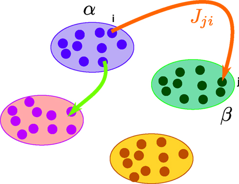
FigureÃÂ 1. General network considered: N neurons belonging to P populations are interconnected with random synaptic weights whose probability distributions only depend upon the population indexes, see text.
Definition 1. The function p: {1,…,N}à→à{1,…,P} associates to each neuron ià∈à{1,…,N}, the population αà=àp(i)à∈à{1,…,P}, it belongs to.
We consider that each neuron i is described by its membrane potential Vi(t), and the related instantaneous firing rate is deduced from it through a relation of the form νi(t)ÃÂ =ÃÂ Si(Vi(t)) (Dayan and Abbott, 2001
; Gerstner and Kistler, 2002
), where Si is a sigmoidal function.
A single action potential from neuron j generates a postsynaptic potential PSPij(u) on the postsynaptic neuron i, where u is the time elapsed after the spike is received. We neglect the delays due to the distance traveled down the axon by the spikes.
Assuming that the postsynaptic potentials sum linearly, the average membrane potential of neuron i is
where the sum is taken over the arrival times of the spikes produced by the neurons j after some reference time t0. The number of spikes arriving between t and tÃÂ +ÃÂ dt is νj(t)dt. Therefore we have
or, equivalently
The PSPijs can depend on several variables in order to account for instance for adaptation or learning.
We now make the simplifying assumption that the shape of the postsynaptic potential PSPij only depends on the postsynaptic population, which corresponds to the voltage-based models in Ermentrout’s (1998)
classification.
The voltage-based model. The assumption, made in Hopfield (1984)
, is that the postsynaptic potential has the same shape no matter which presynaptic population caused it, the sign and amplitude may vary though. This leads to the relation
gi represents the unweighted shape (called a g-shape) of the postsynaptic potentials and  is the strength of the postsynaptic potentials elicited by neuron j on neuron i. At this stage of the discussion, these weights are supposed to be deterministic. This is reflected in the notation which indicates an average value
1
. From Eq.ÃÂ 1 we have
is the strength of the postsynaptic potentials elicited by neuron j on neuron i. At this stage of the discussion, these weights are supposed to be deterministic. This is reflected in the notation which indicates an average value
1
. From Eq.ÃÂ 1 we have
is the strength of the postsynaptic potentials elicited by neuron j on neuron i. At this stage of the discussion, these weights are supposed to be deterministic. This is reflected in the notation which indicates an average value
1
. From Eq.ÃÂ 1 we have
So far we have only considered the synaptic inputs to the neurons. We enrich our model by assuming that the neuron i receives also an external current density composed of a deterministic part, noted Ii(t), and a stochastic part, noted ni(t), so that
We assume, and this is essential for deriving the mean-field equations below, that all indexed quantities depend only upon the P populations of neurons (see Definition 1), i.e.,
where xÃÂ ∼ÃÂ y indicates that the two random variables x and y have the same probability distribution. In other words, all neurons in the same population are described by identical equations (in law).
The g-shapes describe the shape of the postsynaptic potentials and can reasonably well be approximated by smooth functions.
In detail we assume that gα, αà=à1,…,P is the Green function of a linear differential equation of order k, i.e., satisfies

where δ(t) is the Dirac delta function.
The functions blα(t), là=à0,…,k, αà=à1,…,P, are assumed to be continuous. We also assume for simplicity that

for all tÃÂ ∈ÃÂ  We note
  the corresponding differential operator:
We note the corresponding differential operator:
Applying  to both sides of Eq.ÃÂ 3, using Eq.ÃÂ 7 and the fact that νj(s)ÃÂ =ÃÂ Sj(Vj(s)), we obtain a kth-order differential equation for Vi
to both sides of Eq.ÃÂ 3, using Eq.ÃÂ 7 and the fact that νj(s)ÃÂ =ÃÂ Sj(Vj(s)), we obtain a kth-order differential equation for Vi
With a slight abuse of notation, we split the sum with respect to j into P sums:

We classically turn the kth-order differential Eq.ÃÂ 8 into a k-dimensional system of coupled first-order differential equations (we divided both sides of the last equation by ci, see Eq.ÃÂ 6):
A well-known example of g-shapes, see Section “Example II: The model of Jansen and Rit” below or Gerstner and Kistler (2002)
,ÃÂ is

where Y(t) is the Heaviside function. This is an exponentially decaying postsynaptic potential corresponding to
in Eq.ÃÂ 5.
Another well-known example is

This is a somewhat smoother function corresponding to
in Eq.ÃÂ 5.
The dynamics. We modify the Eq.ÃÂ 9 by perturbing the first kÃÂ −ÃÂ 1 equations with Brownian noise and assuming that ni(t) is white noise. This has the effect that the quantities that appear in Eq.ÃÂ 9 are not anymore the derivatives up to order kÃÂ −ÃÂ 1 of Vi. This becomes true again only in the limit where the added Brownian noise is null. This may seem artificial at first glance but (1) it is a technical assumption that is necessary in the proofs of the well-posedness of the mean-field equations, see Assumption 1 below, and (2) it generates a rich class of external stochastic input, as shown below. With this in mind, the Eq.ÃÂ 9 now read

Wli(t), lÃÂ =ÃÂ 0,…,kÃÂ −ÃÂ 1, iÃÂ =ÃÂ 1,…,N, are kN independent standard Brownian processes. Because we want the neurons in the same class to be essentially identical we also assume that the functions fli(t) that control the amount of noise on each derivative satisfy
fli(t)ÃÂ =ÃÂ flp(i)(t), lÃÂ =ÃÂ 0,…,kÃÂ −ÃÂ 1, iÃÂ =ÃÂ 1,…,N
Note that in the limit flα(t)à=à0 for là=à0,…,kà−à1 and αà=à1,…,P, the components Vli(t) of the vector  are the derivatives of the membrane potential Vi, for là=à0,…,kà−à1 and the Eq.à12 turn into Eq.à9. The system of differential Eq.à12 implies that the class of admissible external stochastic input ni(t) to the neuron i are Brownian noise integrated through the filter of the synapse, i.e., involving the lth primitives of the Brownian motion for là≤àk.
are the derivatives of the membrane potential Vi, for là=à0,…,kà−à1 and the Eq.à12 turn into Eq.à9. The system of differential Eq.à12 implies that the class of admissible external stochastic input ni(t) to the neuron i are Brownian noise integrated through the filter of the synapse, i.e., involving the lth primitives of the Brownian motion for là≤àk.We now introduce the kà−à1 N-dimensional vectors Vl(t)à= [Vl1,…,VlN]T, là=à1,…,kà−à1 of the lth-order derivative (in the limit of flp(i)(t)à=à0) of V(t), and concatenate them with V(t) into the Nk-dimensional vector
The N-neurons network is described by the Nk-dimensional vector  . By definition the lth N-dimensional component
  of
of  is equal to Vl. In the limit flα(t)ÃÂ =ÃÂ 0 we have
. By definition the lth N-dimensional component of is equal to Vl. In the limit flα(t)ÃÂ =ÃÂ 0 we have
We next write the equations governing the time variation of the k N-dimensional sub-vectors of , i.e., the derivatives of order 0,…,kÃÂ −ÃÂ 1 of . These are vector versions of Eq.ÃÂ 12. We write
. These are vector versions of Eq.ÃÂ 12. We write
Fl(t) is the Nà×àN diagonal matrix
diag 
where flα(t), αà=à1,…,P is repeated Nα times, and the Wl(t), là=à0,…,kà−à2, are kà−à1 N-dimensional independent standard Brownian processes.
The equation governing the (kà−à1)th differential of the membrane potential has a linear part determined by the differential operators  , αà=à1,…,P and accounts for the external inputs (deterministic and stochastic) and the activity of the neighbors. We note
  the Nà×àNk matrix describing the relation between the neurons membrane potentials and their derivatives up to the order kà−à1 and the (kà−à1)th derivative of V. This matrix is defined as the concatenation of the k Nà×àN diagonal matrixes
, αà=à1,…,P and accounts for the external inputs (deterministic and stochastic) and the activity of the neighbors. We note the Nà×àNk matrix describing the relation between the neurons membrane potentials and their derivatives up to the order kà−à1 and the (kà−à1)th derivative of V. This matrix is defined as the concatenation of the k Nà×àN diagonal matrixesBl(t)à=àdiag
for lÃÂ =ÃÂ 0,…,kÃÂ −ÃÂ 1:
We have:
where Wk−1(t) is an N-dimensional standard Brownian process independent of Wl(t), lÃÂ =ÃÂ 0,…,kÃÂ −ÃÂ 2. The coordinates of the N-dimensional vector I(t) are the external deterministic input currents,
 the Nà×àN matrix of the weights
  which are equal to
  (see Eq.ÃÂ 4), and S is a mapping from
  N to N such that
We define
where IdN is the Nà×àN identity matrix and 0Nà×àN the Nà×àN null matrix. We also define the two kN-dimensional vectors:
where 0N is the N-dimensional null vector.
Combining Eqs.ÃÂ 14 and 15 the full equation satisfied by  can be written:
can be written:
where the kNà×àkN matrix F(t) is equal to diag(F0,…,Fk−1) and Wt is an kN-dimensional standard Brownian process.
The Mean-Field Equations
One of the central goals of this paper is to analyze what happens when we let the total number N of neurons grow to infinity. Can we “summarize” the kN equations (Eq.ÃÂ 17) with a smaller number of equations that would account for the populations activity? We show that the answer to this question is yes and that the populations activity can indeed be represented by P stochastic differential equations of order k. Despite the fact that their solutions are Gaussian processes, these equations turn out to be quite complicated because these processes are non-Markovian.
We assume that the proportions of neurons in each population are nontrivial, i.e.:
If it were not the case the corresponding population would not affect the global behavior of the system, would not contribute to the mean-field equation, and could be neglected.
General derivation of the mean-field equation
When investigating the structure of such mesoscopic neural assemblies as cortical columns, experimentalists are able to provide the average value  of the synaptic efficacy Jij of neural population j to population i. These values are obviously subject to some uncertainty which can be modeled as Gaussian random variables. We also impose that the distribution of the Jijs depends only on the population pair αà=àp(i), βà=àp(j), and on the total number of neurons Nβ of population β:
of the synaptic efficacy Jij of neural population j to population i. These values are obviously subject to some uncertainty which can be modeled as Gaussian random variables. We also impose that the distribution of the Jijs depends only on the population pair αà=àp(i), βà=àp(j), and on the total number of neurons Nβ of population β:
We also make the additional assumption that the Jij’s are independent. This is a reasonable assumption as far as modeling cortical columns from experimental data is concerned. Indeed, it is already difficult for experimentalists to provide the average value of the synaptic strength  from population β to population α and to estimate the corresponding error bars (σαβ), but measuring synaptic efficacies correlations in a large assembly of neurons seems currently out of reach. Though, it is known that synaptic weights are indeed correlated (e.g., via synaptic plasticity mechanisms), these correlations are built by dynamics via a complex interwoven evolution between neurons and synapses dynamics and postulating the form of synaptic weights correlations requires, on theoretical grounds, a detailed investigation of the whole history of neurons–synapses dynamics.
from population β to population α and to estimate the corresponding error bars (σαβ), but measuring synaptic efficacies correlations in a large assembly of neurons seems currently out of reach. Though, it is known that synaptic weights are indeed correlated (e.g., via synaptic plasticity mechanisms), these correlations are built by dynamics via a complex interwoven evolution between neurons and synapses dynamics and postulating the form of synaptic weights correlations requires, on theoretical grounds, a detailed investigation of the whole history of neurons–synapses dynamics.Let us now discuss the scaling form of the probability distribution (Eq.ÃÂ 18) of the Jij’s, namely the division by Nβ for the mean and variance of the Gaussian distribution. This scaling ensures that the “local interaction field”  summarizing the effects of the neurons in population β on neuron i, has a mean and variance which do not depend on Nβ and is only controlled by the phenomenological parameters
  , σαβ.
summarizing the effects of the neurons in population β on neuron i, has a mean and variance which do not depend on Nβ and is only controlled by the phenomenological parameters , σαβ.We are interested in the limit law when NÃÂ →ÃÂ ∞ of the N-dimensional vector V defined in Eq.ÃÂ 3 under the joint law of the connectivities and the Brownian motions, which we call the mean-field limit. This law can be described by a set of P equations, the mean-field equations. As mentioned in the introduction these equations can be derived in several ways, either heuristically as in the work of Amari (Amari, 1972
; Amari et al., 1977
), Sompolinsky (Crisanti et al., 1990
; Sompolinsky et al., 1998
), and Cessac (Cessac, 1995
; Samuelides and Cessac, 2007
), or rigorously as in the work of Ben-Arous and Guionnet (Ben-Arous and Guionnet, 1995
, 1997
; Guionnet, 1997
) . We derive them here in a pedestrian way, prove that they are well-posed, and provide an algorithm for computing their solution.
The effective description of the network population by population is possible because the neurons in each population are interchangeable, i.e., have the same probability distribution under the joint law of the multidimensional Brownian motion and the connectivity weights. This is the case because of the relations (Eqs.ÃÂ 4ÃÂ andÃÂ 16) which imply the form of Eq.ÃÂ 17.
The mean ideas of dynamic mean-field equations. Before diving into the mathematical developments let us comment briefly what are the basic ideas and conclusions of the mean-field approach. Following Eq.ÃÂ 8, the evolution of the membrane potential of some neuron i in population α is given by:
Using the assumption that Si, Ii, ni depend only on neuron population, this gives:
where we have introduced the local interaction field ηiβ(V(t))ÃÂ =ÃÂ  , summarizing the effects of neurons in population β on neuron i and whose probability distribution only depends on the pre- and postsynaptic populations α and β.
, summarizing the effects of neurons in population β on neuron i and whose probability distribution only depends on the pre- and postsynaptic populations α and β.In the simplest situation where the Jij’s have no fluctuations (σαβà=à0) this field reads  . The term Φβ(V(t))à=ÃÂ
. The term Φβ(V(t))ÃÂ =ÃÂ  is the frequency rate of neurons in population β, averaged over this population. Introducing in the same way the average membrane potential in population β,
  , one obtains:
. The term Φβ(V(t))ÃÂ =ÃÂ is the frequency rate of neurons in population β, averaged over this population. Introducing in the same way the average membrane potential in population β, , one obtains:
This equation resembles very much Eq.ÃÂ 19 if one makes the following reasoning: “Since Φβ(V (t) is the frequency rate of neurons in population β, averaged over this population, and since, for one neuron, the frequency rate is νi(t)ÃÂ =ÃÂ Si(Vi(t)) let us write Φβ(V(t))ÃÂ =ÃÂ Sβ(Vβ(t))”. This leads to:
which has exactly the same form as Eq.ÃÂ 19 but at the level of a neuron population. Equations such as (22), which are obtained via a very strong assumption:
are typically those obtained by Jansen and Rit (1995)
. Surprisingly, they are correct and can be rigorously derived, as discussed below, provided σαβà=à0.
However, they cannot remain true, as soon as the synaptic weights fluctuate. Indeed, the transition from Eqs.à19 to 22 corresponds to a projection from a NP-dimensional space to a P-dimensional one, which holds because the NPà×àNP dimensional synaptic weights matrix has in fact only P linearly independent rows. This does not hold anymore if the Jij’s are random and the synaptic weights matrix has generically full rank. Moreover, the effects of the nonlinear dynamics on the synaptic weights variations about their mean, is not small even if the σαβs are and the real trajectories of Eq.à19 can depart strongly from the trajectories of Eq.à22. This is the main message of this paper.
To finish this qualitative description, let us say in a few words what happens to the mean-field equations when σαβà≠à0. We show below that the local interaction fields ηαβ(V (t)) becomes, in the limit Nβà→à∞, a time-dependent Gaussian field Uαβ(t). One of the main results is that this field is non-Markovian, i.e., it integrates the whole history, via the synaptic responses g which are convolution products. Despite the fact that the evolution equation for the membrane potential averaged over a population writes in a very simple form:
it hides a real difficulty, since Uαβ(t) depends on the whole past. Therefore, the introduction of synaptic weights variability leads to a drastic change in neural mass models, as we now develop.
The Mean-Field equations. We note  (respectively
  the set of continuous functions from the real interval [t0, T] (respectively
  . By assigning a probability to subsets of such functions, a continuous stochastic process X defines a positive measure of unit mass on
  (respectively
  . This set of positive measures of unit mass is noted
  (respectively
  .
.
(respectively the set of continuous functions from the real interval [t0, T] (respectively . By assigning a probability to subsets of such functions, a continuous stochastic process X defines a positive measure of unit mass on (respectively . This set of positive measures of unit mass is noted (respectively .We now define a process of particular importance for describing the limit process: the effective interaction process.
Definition 2. (Effective interaction process). Let XÃÂ ∈ÃÂ  (respectively
  be a given Gaussian stochastic process. The effective interaction term is the Gaussian process UXÃÂ ∈ÃÂ
  , (respectively
  ) defined by:
(respectively be a given Gaussian stochastic process. The effective interaction term is the Gaussian process UXÃÂ ∈ÃÂ , (respectively ) defined by:
where
and

In order to construct the solution of the mean-field equations (see Section “Existence and Uniqueness of Solutions in Finite Time”) we will need more explicit expressions for  and
and  which we obtain in the next proposition.
and which we obtain in the next proposition.Proposition 1. Let  be the mean of the process XÃÂ and
  be its covariance matrix. The vectors mX(t) and ΔX(t, s) that appear in the definition of the effective interaction process UX are defined by the following expressions:
be the mean of the process XÃÂ and be its covariance matrix. The vectors mX(t) and ΔX(t, s) that appear in the definition of the effective interaction process UX are defined by the following expressions:
and
where
is the probability density of a 0-mean, unit variance, Gaussian variable.
Proof. The results follow immediately by a change of variable from the fact that Xβ(t) is a univariate Gaussian random variable of mean μβ(t) and variance Cββ(t, t) and the pair (Xβ(t), Xβ(s)) is bivariate Gaussian random variable with mean (μβ(t), μβ(s)) and covariance matrix

Choose P neurons i1,…,iP, one in each population (neuron iα belongs to the population α). We define the kP-dimensional vector  by choosing, in each of the k N-dimensional components
  , of the vector
  defined in Eq.ÃÂ 13 the coordinates of indexes i1,…,iP. Then it can be shown, using either a heuristic argument or large deviations techniques (see Appendix A), that the sequence of kP-dimensional processes
  converges in law to the process
  solution of the following mean-field equation:
by choosing, in each of the k N-dimensional components , of the vector defined in Eq.ÃÂ 13 the coordinates of indexes i1,…,iP. Then it can be shown, using either a heuristic argument or large deviations techniques (see Appendix A), that the sequence of kP-dimensional processes converges in law to the process solution of the following mean-field equation:
L is the Pkà×àPk matrix
The Pà×àP matrixes Bl(t), là=à0,…,kà−à1 are, with a slight abuse of notations, equal to diag(bl1(t),…,blP(t)).  is a kP-dimensional standard Brownian process.
  has the law of the P-dimensional effective interaction vector associated to the vector
  (first P-dimensional component of
  ) and is statistically independent of the external noise
  and of the initial condition
  (when t0ÃÂ >ÃÂ −∞):
is a kP-dimensional standard Brownian process. has the law of the P-dimensional effective interaction vector associated to the vector (first P-dimensional component of ) and is statistically independent of the external noise and of the initial condition (when t0ÃÂ >ÃÂ −∞):
We have used for the matrixes Fl(t), lÃÂ =ÃÂ 0,…,kÃÂ −ÃÂ 1 the same abuse of notations as for the matrixes Bl(t), i.e., Fl(t)ÃÂ =ÃÂ diag(fl1(t),…,flP(t)) for lÃÂ =ÃÂ 0,…,kÃÂ −ÃÂ 1. I(t) is the P-dimensional external current [I1(t),…,IP(t)]T.
The process  is a Pà×àP-dimensional process and is applied, as a matrix, to the P-dimensional vector 1 with all coordinates equal to 1, resulting in the P-dimensional vector
  whose mean and covariance function can be readily obtained from Definition 2:
is a Pà×àP-dimensional process and is applied, as a matrix, to the P-dimensional vector 1 with all coordinates equal to 1, resulting in the P-dimensional vector whose mean and covariance function can be readily obtained from Definition 2:
and
We have of course
Equations (28) are formally very similar to Eq.ÃÂ 17 but there are some very important differences. The first ones are of dimension kP whereas the second are of dimension kN which grows arbitrarily large when NÃÂ →ÃÂ ∞. The interaction term of the second,  is simply the synaptic weight matrix applied to the activities of the N neurons at time t. The interaction term of the first equation,
  , though innocuous looking, is in fact quite complex (see Eqs.ÃÂ 29ÃÂ andÃÂ 30). In fact the stochastic process
  , putative solution of Eq.ÃÂ 28, is in general non-Markovian.
is simply the synaptic weight matrix applied to the activities of the N neurons at time t. The interaction term of the first equation, , though innocuous looking, is in fact quite complex (see Eqs.ÃÂ 29ÃÂ andÃÂ 30). In fact the stochastic process , putative solution of Eq.ÃÂ 28, is in general non-Markovian.To proceed further we formally integrate the equation using the flow, or resolvent, of the Eq.ÃÂ 28, noted ΦL(t, t0) (see AppendixÃÂ B), and we obtain, since we assumed L continuous, an implicit representation of  :
:
:
We now introduce for future reference a simpler model which is quite frequently used in the description on neural networks and has been formally analyzed by Sompolinsky and colleagues (Crisanti et al., 1990
; Sompolinsky et al., 1998
) in the case of one population (PÃÂ =ÃÂ 1).
Example I: The Simple Model
In the Simple Model, each neuron membrane potential decreases exponentially to its rest value if it receives no input, with a time constant τα depending only on the population. In other words, we assume that the g-shape describing the shape of the PSPs is Eq.ÃÂ 10, with KÃÂ =ÃÂ 1 for simplicity. The noise is modeled by an independent Brownian process per neuron whose standard deviation is the same for all neurons belonging to a given population.
Hence the dynamics of a given neuron i from population α of the network reads:
This is a special case of Eq.à12 where kà=à1, b0α(t)à=à1/τα, b1α(t)à=à1 for αà=à1,…,P. The corresponding mean-field equation reads:
where the processes (Wα(t))tà≥àt0 are independent standard Brownian motions,  is the effective interaction term, see Definition 2. This is a special case of Eq.à28 with Là= diag(
is the effective interaction term, see Definition 2. This is a special case of Eq.ÃÂ 28 with LÃÂ = diag( ), and FÃÂ =ÃÂ diag(f1,…,fP).
is the effective interaction term, see Definition 2. This is a special case of Eq.ÃÂ 28 with LÃÂ = diag(), and FÃÂ =ÃÂ diag(f1,…,fP).Taking the expected value of both sides of Eq.ÃÂ 33 and using we obtain Eq.ÃÂ 26 that the mean μα(t) of α(t) satisfies the differential equation
α(t) satisfies the differential equation
If Cββ(t, t) vanishes for all tà≥àt0 this equation reduces to:
which is precisely the “naive” mean-field equation (Eq.à22) obtained with the assumption (Eq.à23). We see that Eq.à22 are indeed correct, provided that Cββ(t, t)à=à0, ∀tà≥àt0.
EquationÃÂ 33 can be formally integrated implicitly and we obtain the following integral representation of the process α(t):
α(t):
where t0 is the initial time. It is an implicit equation on the probability distribution of (t), a special case of (Eq.ÃÂ 31), with 
(t), a special case of (Eq.ÃÂ 31), with The variance Cαα(t, t) of α(t) can easily be obtained from Eq.ÃÂ 34. It reads
α(t) can easily be obtained from Eq.ÃÂ 34. It reads
where Δβ(u, v) is given by Eq.ÃÂ 27.
If σαβà=à0 and if sαà=à0 then Cαα(t, t)à=à0, ∀tà≥àt0 is a solution of this equation. Thus, mean-field equations for the simple model reduce to the naive mean-field Eq.à22 in this case. This conclusion extends as well to all models of synaptic responses, ruled by Eq.à5.
However, the equation of Cαα(t, t) shows that, in the general case, in order to solve the differential equation for μα(t), we need to know the whole past of the process . This exemplifies a previous statement on the non-Markovian nature of the solution of the mean-field equations.
. This exemplifies a previous statement on the non-Markovian nature of the solution of the mean-field equations.Example II: The model of Jansen and Rit
One of the motivations of this study is to characterize the global behavior of an assembly of neurons in particular to get a better understanding of recordings of cortical signals like EEG or MEG. One of the classical models of neural masses is Jansen and Rit’s mass model (Jansen and Rit, 1995
), in short the JR model (see Figure 2
).
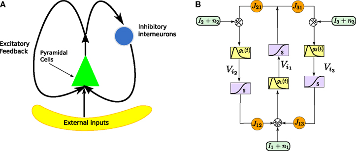
FigureÃÂ 2. (A) Neural mass model: a population of pyramidal cells interacts with itself in an excitatory mode and with an inhibitory population of inter-neurons. (B) Block representation of the model. The g boxes account for the synaptic integration between neuronal populations. S boxes simulate cell bodies of neurons by transforming the membrane potential of a population into an output firing rate. The coefficients Jαβ are the random synaptic efficiency of population β on population α (1 represents the pyramidal population, 2 the excitatory feedback, and 3 the inhibitory inter-neurons).
The model features a population of pyramidal neurons that receives inhibitory inputs from local inter-neurons, excitatory feedbacks, and excitatory inputs from neighboring cortical units and sub-cortical structures such as the thalamus. The excitatory input is represented by an external firing rate that has a deterministic part I1(t) accounting for specific activity of other cortical units and a stochastic part n1(t) accounting for a non specific background activity. We formally consider that the excitatory feedback of the pyramidal neurons is a new neural population, making the number P of populations equal to 3. We also represent the external inputs to the other two populations by the sum of a deterministic part Ij(t) and a stochastic part nj(t), jÃÂ =ÃÂ 2, 3, see Figure 2
.
In the model introduced originally by Jansen and Rit, the connectivity weights were assumed to be constant, i.e., equal to their mean value. Nevertheless, there exists a variability of these coefficients, and as we show in the sequel, the effect of the connectivity variability impacts the solution at the level of the neural mass. Statistical properties of the connectivities have been studied in details for instance in (Braitenberg and Schüz, 1998
).
We consider a network of N neurons, Nα, αà=à1, 2, 3 belonging to population α. We index by 1 (respectively 2, and 3) the pyramidal (respectively excitatory feedback, inhibitory interneuron) populations. We choose in each population a particular neuron indexed by iα, αà=à1, 2, 3. The evolution equations of the network can be written for instance in terms of the potentials Vi1, Vi2 and Vi3 labeled in Figure 2 and these equations read:
In the mean-field limit, denoting by α, αà=à1, 2, 3 the average membrance potential of each class, we obtain the following equations:
α, αà=à1, 2, 3 the average membrance potential of each class, we obtain the following equations:
where  is the effective interaction process associated with this problem, i.e., a Gaussian process of mean:
is the effective interaction process associated with this problem, i.e., a Gaussian process of mean:
All other mean values correspond to the non-interacting populations and are equal to 0. The covariance matrix can be deduced from Eq.ÃÂ 25:
where
This model is a voltage-based model in the sense of Ermentrout (1998)
. Let us now instantiate the synaptic dynamics and compare the mean-field equations with Jansen’s population equations
2
(sometimes improperly called also mean-field equations).
The simplest model of synaptic integration is a first-order integration, which yields exponentially decaying postsynaptic potentials:
Note that this is exactly Eq.ÃÂ 10. The corresponding g-shape satisfies the following first-order differential equation
In this equation τ is the time constant of the synaptic integration and K the synaptic efficiency. The coefficients K and τ are the same for the pyramidal and the excitatory feedback population (characteristic of the pyramidal neurons and defining the g-shape g1), and different for the inhibitory population (defining the g-shape g3). In the pyramidal or excitatory (respectively the inhibitory) case we have Kà=àK1, τà=àτ1 (respectively Kà=àK3, τà=àτ3). Finally, the sigmoid functions S is given by
where νmax is the maximum firing rate, and v0 is a voltage reference.
With this synaptic dynamics we obtain the first-order Jansen and Rit’s equation:
The “original” Jansen and Rit’s equation (Grimbert and Faugeras, 2006
; Jansen and Rit, 1995
) amount considering only the mean of the process and assuming that  for i, jÃÂ ∈ÃÂ {1, 2, 3}, i.e., that the expectation commutes with the sigmoidal function S. This is a very strong assumption, and that the fluctuations of the solutions of the mean-field equation around the mean imply that the sigmoid cannot be considered as linear in the general case.
and assuming that for i, jÃÂ ∈ÃÂ {1, 2, 3}, i.e., that the expectation commutes with the sigmoidal function S. This is a very strong assumption, and that the fluctuations of the solutions of the mean-field equation around the mean imply that the sigmoid cannot be considered as linear in the general case.A higher order model was introduced by van Rotterdam et al. (1982)
to better account for the synaptic integration and to better reproduce the characteristics of real postsynaptic potentials. In this model the g-shapes satisfy a second-order differential equation:
We recognize the g-shape defined by Eq.ÃÂ 11 solution of the second-order differential equation  With this type of synaptic integration, we obtain the following mean-field equations:
With this type of synaptic integration, we obtain the following mean-field equations:
Here again, going from the mean-field Eq.ÃÂ 37 to the original Jansen and Rit’s neural mass model consists in studying the equation of the mean of the process given by Eq.ÃÂ 37 and commuting the sigmoidal function with the expectation.
Note that the introduction of higher order synaptic integrations results in richer behaviors. For instance, Grimbert and Faugeras (2006)
showed that some bifurcations can appear in the second-order JR model giving rise to epileptic like oscillations and alpha activity, that do not appear in the first-order model.
The mean-field equation (Eq.à31) is an implicit equation of the stochastic process (V(t))tà≥àt0. We prove in this section that under some mild assumptions this implicit equation has a unique solution. These assumptions are the following.
Assumption 1.
(a) The matrix L(t) is C0 and satisfies ‖L(t)‖à≤àkL for all t in [t0,àT], for some matrix norm ‖ ‖ and some strictly positive constantàkL.
(b) The matrix F(t) has all its singular values lowerbounded (respectively upperbounded) by the strictly positive constant
3
 (respectively
  ) for all t in [t0, T].
(respectively ) for all t in [t0, T].(c) The deterministic external input vector I(t) is bounded and we have ‖I(t)‖∞à≤àImax for all t in [t0, T] and some strictly positive constant Imax.
This solution is the fixed point in the set  of kP-dimensional processes of an equation that we will define from the mean-field equations. We will construct a sequence of Gaussian processes and prove that it converges in distribution toward this fixed point.
of kP-dimensional processes of an equation that we will define from the mean-field equations. We will construct a sequence of Gaussian processes and prove that it converges in distribution toward this fixed point.We first recall some results on the convergence of random variables and stochastic processes.
Convergence of Gaussian Processes
We recall the following result from Bogachev (1998)
which formalizes the intuition that a sequence of Gaussian processes converges toward a Gaussian process if and only if the means and covariance functions converge. In fact in order for this to be true, it is only necessary to add one more condition, namely that the corresponding sequence of measures (elements of  ) do not have “any mass at infinity”. This property is called uniform tightness (Billingsley, 1999
). More precisely we have
) do not have “any mass at infinity”. This property is called uniform tightness (Billingsley, 1999
). More precisely we have
) do not have “any mass at infinity”. This property is called uniform tightness (Billingsley, 1999
). More precisely we haveDefinition 3. (Uniform tightness). Let  be a sequence of kP-dimensional processes defined on [t0, T] and Pn be the associated elements of
  . The sequence
  is called uniformly tight if and only if for all εà>à0 there exists a compact set K of
  such that Pn(K)à>à1à−àε, nà≥à1.
be a sequence of kP-dimensional processes defined on [t0, T] and Pn be the associated elements of . The sequence is called uniformly tight if and only if for all εà>à0 there exists a compact set K of such that Pn(K)à>à1à−àε, nà≥à1.Theorem 1. Let  be a sequence of kP-dimensional Gaussian processes defined on [t0, T] or on an unbounded interval
4
of . The sequence converges to a Gaussian process X if and only if the following three conditions are satisfied:
be a sequence of kP-dimensional Gaussian processes defined on [t0, T] or on an unbounded interval
4
of . The sequence converges to a Gaussian process X if and only if the following three conditions are satisfied:
be a sequence of kP-dimensional Gaussian processes defined on [t0, T] or on an unbounded interval
4
of . The sequence converges to a Gaussian process X if and only if the following three conditions are satisfied:• The sequence  is uniformly tight.
is uniformly tight.• The sequence μn(t) of the mean functions converges for the uniform norm.
• The sequence Cn of the covariance operators converges for the uniform norm.
We now, as advertised, define such a sequence of Gaussian processes.
Let us fix Z0, a kP-dimensional Gaussian random variable, independent of the Brownian and of the process ((X)t)tÃÂ ∈ÃÂ [t0,T].
Definition 4. Let X be an element of  and
and  beÃÂ the function
  such that
and beÃÂ the function such that
where  and
and  are defined
5
in Section “Mean-Field Equations for Multi-Populations Neural Network Models”.
are defined
5
in Section “Mean-Field Equations for Multi-Populations Neural Network Models”.
and are defined
5
in Section “Mean-Field Equations for Multi-Populations Neural Network Models”.Note that, by Definition 2 the random process ((X))tà∈ [t0,àT], kà≥à1 is the sum of a deterministic function (defined by the external current) and three independent random processes defined by Z0, the interaction between neurons, and the external noise. These three processes being Gaussian processes, so is ((X))tà∈à[t0,àT]. Also note that ((X))t0à=àZ0. It should be clear that a solution of the mean-field equation (Eq.à31) satisfies (t0)à=àZ0 and is a fixed point of , i.e., ()tà=à(t).
(X))tà∈ [t0,àT], kà≥à1 is the sum of a deterministic function (defined by the external current) and three independent random processes defined by Z0, the interaction between neurons, and the external noise. These three processes being Gaussian processes, so is ((X))tà∈à[t0,àT]. Also note that ((X))t0à=àZ0. It should be clear that a solution of the mean-field equation (Eq.à31) satisfies (t0)à=àZ0 and is a fixed point of , i.e., ()tà=à(t).Let X be a given stochastic process of  such that
  (hence
  is independent of the Brownian). We define the sequence of Gaussian processes
  by:
by:
such that (hence is independent of the Brownian). We define the sequence of Gaussian processes by:
In the remaining of this section we show that the sequence of processes  converges in distribution toward the unique fixed-point Y of which is also the unique solution of the mean-field equation (Eq.ÃÂ 31).
converges in distribution toward the unique fixed-point Y of which is also the unique solution of the mean-field equation (Eq.ÃÂ 31).Existence and uniqueness of a solution for the mean-field equations
The following upper and lower bounds are used in the sequel.
Lemma 1. Consider the Gaussian process  UX is defined in Sections “The Mean-Field Equations” and “Introduction” is the Pdimensional vector with all coordinates equal to 1. We have
UX is defined in Sections “The Mean-Field Equations” and “Introduction” is the Pdimensional vector with all coordinates equal to 1. We have
for all t0à≤àtà≤àT. The maximum eigenvalue of its covariance matrix is upperbounded by  where ‖Sβ‖∞ is the supremum of the absolute value of Sβ. We also note
where ‖Sβ‖∞ is the supremum of the absolute value of Sβ. We also note Proof. The proof is straightforward from Definition 4.
The proof of existence and uniqueness of solution, and of the convergence of the sequence (Eq.à38) is in two main steps. We first prove that the sequence of Gaussian processes  , kà≥à1 is uniformly tight by proving that it satisfies Kolmogorov’s criterion for tightness. This takes care of condition 1 in Theorem 1. We then prove that the sequences of the mean functions and covariance operators are Cauchy sequences for the uniform norms, taking care of conditions 2 and 3.
, kà≥à1 is uniformly tight by proving that it satisfies Kolmogorov’s criterion for tightness. This takes care of condition 1 in Theorem 1. We then prove that the sequences of the mean functions and covariance operators are Cauchy sequences for the uniform norms, taking care of conditions 2 and 3.Uniform tightness
We first recall the following theorem due to Kolmogorov (Kushner, 1984
, Chapter 4.1).
Theorem 2. (Kolmogorov’s criterion for tightness). Let  be a sequence of kP-dimensional processes defined on [t0, T]. If there exist α, β, CÃÂ >ÃÂ 0 such that
be a sequence of kP-dimensional processes defined on [t0, T]. If there exist α, β, CÃÂ >ÃÂ 0 such that
then the sequence is uniformly tight.
Using this theorem we prove that the sequence  , kà≥à1 satisfies Kolmogorov’s criterion for βà=à4 and αà≥à1. The reason for choosing βà=à4 is that, heuristically, dWà.à(dt)1/2. Therefore in order to upperbound
  by a power of | tà−às |à≥à2 (hence strictly larger than 1) we need to raise
  to a power at least equal to 4. The proof itself is technical and uses standard inequalities (Cauchy–Schwarz’s and Jensen’s), properties of Gaussian integrals, elementary properties of the stochastic integral, and Lemma 1. It also uses the fact that the input currentàis bounded, i.e., that
to a power at least equal to 4. The proof itself is technical and uses standard inequalities (Cauchy–Schwarz’s and Jensen’s), properties of Gaussian integrals, elementary properties of the stochastic integral, and Lemma 1. It also uses the fact that the input currentÃÂ is bounded, i.e., that  this is Assumption (c) in 1.
, kà≥à1 satisfies Kolmogorov’s criterion for βà=à4 and αà≥à1. The reason for choosing βà=à4 is that, heuristically, dWà.à(dt)1/2. Therefore in order to upperbound by a power of | tà−às |à≥à2 (hence strictly larger than 1) we need to raise to a power at least equal to 4. The proof itself is technical and uses standard inequalities (Cauchy–Schwarz’s and Jensen’s), properties of Gaussian integrals, elementary properties of the stochastic integral, and Lemma 1. It also uses the fact that the input currentàis bounded, i.e., that this is Assumption (c) in 1.Theorem 3. The sequence of processes  , kà≥à1 is uniformly tight.
, kà≥à1 is uniformly tight.Proof. We do the proof for kà=à1, the case kà>à1 is similar. If we assume that nà≥à1 and sà<àt we can rewrite the difference  as follows, using property (i) in PropositionàB.1 in Appendix B.
as follows, using property (i) in PropositionÃÂ B.1 in Appendix B.
as follows, using property (i) in PropositionÃÂ B.1 in Appendix B.
The righthand side is the sum of seven terms and therefore (Cauchy–Schwarz inequality):
Because ‖ΦL(t, t0)à−àΦL(s, t0)‖à≤à|tà−às| ‖L ‖we see that all terms in the righthand side of the inequality but the second one involving the Brownian motion are of the order of (tà−às)2. We raise again both sides to the second power, use the Cauchy–Schwarz inequality, and take the expected value:
Remember that  is a P-dimensional diagonal Gaussian process, noted Yu in the sequel, therefore:
is a P-dimensional diagonal Gaussian process, noted Yu in the sequel, therefore:
The second-order moments are upperbounded by some regular function of μ and σmax (defined in Lemma 1) and, because of the properties of Gaussian integrals, so are the fourth-order moments.
We now define B(u)ÃÂ =ÃÂ ΦL(s, u)F(u) and evaluate  We have
We have
Because  is by construction independent of
  if ià≠àj and
  for all i, j (property of the It integral), the last term is the sum of only three types of terms:
is by construction independent of if ià≠àj and for all i, j (property of the It integral), the last term is the sum of only three types of terms:1. If j1à=àk1à=àj2à=àk2 we define
and, using Cauchy–Schwarz:
2. If j1à=àk1 and j2à=àk2 but 1à≠àj2 we define
which is equal, because of the independence of  and
and  to
to
and to
3. Finally, if j1à=àj2 and k1à=àk2 but j1à≠àk1 we define
which is equal, because of the independence of  and
and  to
to
and to
because of the properties of the stochastic integral,
 hence, because of the properties of the Gaussian integrals
hence, because of the properties of the Gaussian integrals
for some positive constant k. This takes care of the terms of the form T1. Next we have
which takes care of the terms of the form T2. Finally we have, because of the properties of the It integral
which takes care of the terms of the form T3.
This shows that the term  in Eq.à40 is of the order of (tà−às)1+a where aà≥à1. Therefore we have
in Eq.à40 is of the order of (tà−às)1+a where aà≥à1. Therefore we have
for all s, t in [t0, T], where C is a constant independent of t, s. According to Kolmogorov criterion for tightness, the sequence of processes  is uniformly tight.
is uniformly tight.The proof for , kÃÂ >ÃÂ 1 is similar.
, kÃÂ >ÃÂ 1 is similar. The mean and covariance sequences are Cauchy sequences
Let us note μn(t) [respectively Cn(t, s)] the mean (respectively the covariance matrix) function of Xnà=à(Xn−1), nà≥à1. We have:
(Xn−1), nà≥à1. We have:
where  is given by Eq.ÃÂ 26. Similarly we have
is given by Eq.ÃÂ 26. Similarly we have
Note that the kPà×àkP covariance matrix  has only one nonzero Pà×àP block:
has only one nonzero Pà×àP block:
According to Definition 2 we have
where  is given by Eq.ÃÂ 27 and Dx is defined in PropositionÃÂ 1.
is given by Eq.à27 and Dx is defined in Propositionà1.In order to prove our main result, that the two sequences of functions (μn) and (Cn) are uniformly convergent, we require the following four lemmas that we state without proofs, the proofs being found in Appendixes E–H. The first lemma gives a uniform (i.e., independent of nà≥à2 and αà=à1,…,kP) strictly positive lowerbound for  In what follows we use the following notation: Let C be a symmetric positive definite matrix, we note
  its smallest eigenvalue.
In what follows we use the following notation: Let C be a symmetric positive definite matrix, we note its smallest eigenvalue.Lemma 2. The following uppperbounds are valid for all nà≥à1 and all s, tà∈à[t0, T].

where μ and σmax are defined in Lemma 1,  is defined in Assumption 1.
is defined in Assumption 1.Lemma 3. For all t ∈ [t0, T] all αà=à1,…,kP, and nà≥à1, we have
where λmin is the smallest singular value of the positive symmetric definite matrix ΦL(t, t0)ΦL(t, t0)T for tÃÂ ∈ÃÂ [t0, T] and  is the smallest eigenvalue of the positive symmetric definite covariance matrix
  .
.
is the smallest eigenvalue of the positive symmetric definite covariance matrix .The second lemma also gives a uniform lowerbound for the expression  which appears in the definition of Cn+1 through Eqs.ÃÂ 43ÃÂ andÃÂ 27. The crucial point is that this function is O(|tÃÂ −ÃÂ s|) which is central in the proof of Lemma 5.
which appears in the definition of Cn+1 through Eqs.à43àandà27. The crucial point is that this function is O(|tà−às|) which is central in the proof of Lemma 5.Lemma 4. For all αà=à1,…,kP and nà≥à1 the quantity  is lowerbounded by the positive symmetric function:
is lowerbounded by the positive symmetric function:
where  is the strictly positive lower bound, introduced in Assumption 1, on the singular values of the matrix F(u) for u ∈ [t0, T].
is the strictly positive lower bound, introduced in Assumption 1, on the singular values of the matrix F(u) for u ∈ [t0, T].The third lemma shows that an integral that appears in the proof of the uniform convergence of the sequences of functions (μn) and (Cn) is upperbounded by the nth term of a convergent series.
Lemma 5. The 2n-dimensional integral
where the functions ρi(ui, vi), iÃÂ =ÃÂ 1,…,n are either equal to 1 or to  (the function θ is defined in Lemma 4), is upperbounded by kn/(nÃÂ −ÃÂ 1)! for some positive constant k.
(the function θ is defined in Lemma 4), is upperbounded by kn/(nÃÂ −ÃÂ 1)! for some positive constant k.With these lemmas in hand we prove Proposition 3. The proof is technical but its idea is very simple. We find upperbounds for the matrix infinite norm of Cn+1(t, s)ÃÂ −ÃÂ Cn(t, s) and the infinite norm of μn+1(t)ÃÂ −ÃÂ μn(t) by applying the mean value Theorem and LemmasÃÂ 3 and 4 to the these norms. These upperbounds involve integrals of the infinite norms of Cn(t, s)ÃÂ −ÃÂ Cn−1(t, s) and μn(t)ÃÂ −ÃÂ μn−1(t) and, through Lemma 4, one over the square root of the function θ. Proceeding recursively and using Lemma 5, one easily shows that the infinite norms of Cn+1ÃÂ −ÃÂ Cn and μn+1ÃÂ −ÃÂ μn are upperbounded by the nth term of a convergent series from which it follows that the two sequences of functions are Cauchy sequences, hence convergent.
Proposition 3. The sequences of covariance matrix functions Cn(t,ÃÂ s) and of mean functions μn(t), s, t in [t0, T] are Cauchy sequences for the uniform norms.
Proof. We have
We take the infinite matrix norm of both sides of this equality and use the upperbounds  and
and  (see Appendix B) to obtain
6
(see Appendix B) to obtain
6
and (see Appendix B) to obtain
6
According to Eq.ÃÂ 27 we are led to consider the difference AnÃÂ −ÃÂ An−1, where:
We write next:
The mean value theorem yields:

Using the fact that  , we obtain:
, we obtain:
where the constants kL and  are defined in Appendix B and
are defined in Appendix B and
A similar process applied to the mean values yields:
where μ is defined in Lemma 1. We now use the mean value Theorem and Lemmas 3 and 4 to find upperbounds for 
 and
and  We have
and We have
where k0 is defined in Lemma 3. Hence:
Along the same lines we can show easily that:
and that:
where θ(u, v) is defined in Lemma 4. Grouping terms together and using the fact that all integrated functions are positive, we write:
Note that, because of Lemma 3, all integrals are well-defined. Regarding the mean functions, we write:
Proceeding recursively until we reach C0 and μ0 we obtain an upperbound for ‖Cn+1(t, s) − Cn(t, s)‖∞ (respectively for ‖μn+1(t)ÃÂ −ÃÂ μn(t)‖∞) which is the sum of <5n terms each one being the product of k raised to a power ≤n, times 2μmax or 2Σmax (upperbounds for the norms of the mean vector and the covariance matrix defined in Lemma 2), times a 2n-dimensional integral In given by
where the functions ρi(ui, vi), iÃÂ =ÃÂ 1,…,n are either equal to 1 or to  . According to Lemma 5, this integral is of the order of some positive constant raised to the power n divided by (n −ÃÂ 1)!. Hence the sum is less than some positive constant k raised to the power n divided by (nÃÂ −ÃÂ 1)!. By taking the supremum with respect to t and s in [t0, T] we obtain the same result for ‖Cn+1ÃÂ −ÃÂ Cn‖∞ (respectively for ‖μn+1ÃÂ −ÃÂ μn‖∞). Since the series
  is convergent, this implies that ‖Cn+pÃÂ −ÃÂ Cn‖∞ (respectively ‖μn+pÃÂ −ÃÂ μn‖∞) can be made arbitrarily small for large n and p and the sequence Cn (respectively μn) is a Cauchy sequence.
. According to Lemma 5, this integral is of the order of some positive constant raised to the power n divided by (n −ÃÂ 1)!. Hence the sum is less than some positive constant k raised to the power n divided by (nÃÂ −ÃÂ 1)!. By taking the supremum with respect to t and s in [t0, T] we obtain the same result for ‖Cn+1ÃÂ −ÃÂ Cn‖∞ (respectively for ‖μn+1ÃÂ −ÃÂ μn‖∞). Since the series is convergent, this implies that ‖Cn+pÃÂ −ÃÂ Cn‖∞ (respectively ‖μn+pÃÂ −ÃÂ μn‖∞) can be made arbitrarily small for large n and p and the sequence Cn (respectively μn) is a Cauchy sequence. Existence and uniqueness of a solution of the mean-field equations
It is now easy to prove our main result, that the mean-field equations (Eq.ÃÂ 31) or equivalently (Eq.ÃÂ 28) are well-posed, i.e., have a unique solution.
Theorem 4. For any nondegenerate kP-dimensional Gaussian random variable Z0, independent of the Brownian, and any initial process X such that X(t0)ÃÂ =ÃÂ Z0, the map has a unique fixed point in  toward which the sequence
  of Gaussian processes converges in law.
has a unique fixed point in toward which the sequence of Gaussian processes converges in law.Proof. Since  (respectively
  is a Banach space for the uniform norm, the Cauchy sequence μn (respectively Cn) of Proposition 3 converges to an element μ of
  (respectively an element C of
  . Therefore, according to Theorem 1, the sequence
  of Gaussian processes converges in law toward the Gaussian process Y with mean function μ and covariance function C. This process is clearly a fixed point of .
(respectively is a Banach space for the uniform norm, the Cauchy sequence μn (respectively Cn) of Proposition 3 converges to an element μ of (respectively an element C of . Therefore, according to Theorem 1, the sequence of Gaussian processes converges in law toward the Gaussian process Y with mean function μ and covariance function C. This process is clearly a fixed point of .Hence we know that there exists at least one fixed point for the map . Assume there exist two distinct fixed points Y1 and Y2 of with mean functions μi and covariance functions Ci, ià=à1, 2, with the same initial condition. Since for all nà≥à1 we have  the proof of Proposition 3 shows that
  (respectively
  ) is upperbounded by the product of a positive number an (respectively bn) with ‖μ1ÃÂ −ÃÂ μ2‖∞) (respectively with (‖C1ÃÂ −ÃÂ C2‖∞). Since limn→∞ anÃÂ =ÃÂ limn→∞ bnÃÂ =ÃÂ 0 and
  , iÃÂ =ÃÂ 1, 2 (respectively
  , iÃÂ =ÃÂ 1, 2), this shows that μ1ÃÂ =ÃÂ μ2 and C1ÃÂ =ÃÂ C2, hence the two Gaussian processes Y1 and Y2 are indistinguishable.
. Assume there exist two distinct fixed points Y1 and Y2 of with mean functions μi and covariance functions Ci, ià=à1, 2, with the same initial condition. Since for all nà≥à1 we have the proof of Proposition 3 shows that (respectively ) is upperbounded by the product of a positive number an (respectively bn) with ‖μ1à−àμ2‖∞) (respectively with (‖C1à−àC2‖∞). Since limn→∞ anà=àlimn→∞ bnà=à0 and , ià=à1, 2 (respectively , ià=à1, 2), this shows that μ1à=àμ2 and C1à=àC2, hence the two Gaussian processes Y1 and Y2 are indistinguishable. We have proved that for any nondegenerate Gaussian initial condition Z0 there exists a unique solution of the mean-field equations. The proof of Theorem 4 is constructive, and hence provides a way for computing the solution of the mean-field equations by iterating the map defined in 3.2, starting from any initial process X satisfying X(t0)à=àZ0, for instance a Gaussian process such as an Ornstein–Uhlenbeck process. We build upon these facts in Section “Numerical Experiments”.
defined in 3.2, starting from any initial process X satisfying X(t0)ÃÂ =ÃÂ Z0, for instance a Gaussian process such as an Ornstein–Uhlenbeck process. We build upon these facts in Section “Numerical Experiments”.Note that the existence and uniqueness is true whatever the initial time t0 and the final time T.
So far, we have investigated the existence and uniqueness of solutions of the mean-field equation for a given initial condition. We are now interested in investigating stationary solutions, which allow for some simplifications of the formalism.
A stationary solution is a solution whose probability distribution does not change under the flow of the equation. These solutions have been already investigated by several authors (see Brunel and Hakim, 1999
; Sompolinsky et al., 1998
). We propose a new framework to study and simulate these processes. Indeed we show in this section that under a certain contraction condition there exists a unique solution to the stationary problem. As in the previous section our proof is constructive and provides a way to simulate the solutions.
Remark. The long-time mean-field description of a network is still a great endeavor in mathematics and statistical physics. In this section we formally take the mean-field equation we obtained and let t0ÃÂ →ÃÂ −∞. This way we obtain an equation which is the limit of the mean-field equation when t0ÃÂ →ÃÂ −∞. It means that we consider first the limit NÃÂ →ÃÂ ∞ and then t0ÃÂ →ÃÂ −∞. These two limits do not necessarily commute and there are known examples, for instance in spin-glasses, where they do not.
It is clear that in order to get stationary solutions, the stochastic system has to be autonomous. More precisely, we modify Assumption 1 as follows
Assumption 2.
(a) The matrixes L(t) and F(t), the input currents I(t) do not depend upon t.
(b) The real parts of the eigenvalues of L are negative:

for all eigenvalues λ of L.
(c) The matrix F has full rank.
Under Assumption (a) of 2, the resolvent ΦL(t, s) is equal to eL(t−s). Under Assumption (b) we only consider first-order system since otherwise the matrix L has eigenvalues equal to 0. We now prove the following proposition.
Proposition 4. Under the previous assumptions we have:
1.
2. the process  is well-defined, Gaussian and stationary when t0ÃÂ →ÃÂ −∞.
is well-defined, Gaussian and stationary when t0ÃÂ →ÃÂ −∞.Proof. The first point property follows from the fact that Re(λ)ÃÂ <ÃÂ −λL for all eigenvalues λ of L. This assumption also implies that there exists a norm on P such that
P such that
and hence

for some positive constant k. This implies the remaining two properties.
We now address the second point of the property. The stochastic integral  is well-defined ∀tà≤àT and is Gaussian with 0-mean. Its covariance matrix reads:
is well-defined ∀tà≤àT and is Gaussian with 0-mean. Its covariance matrix reads:
Let us assume for instance that tquotidnÃÂ <ÃÂ t and perform the change of variable uÃÂ =ÃÂ tÃÂ −ÃÂ s to obtain
Under the previous assumptions this matrix integral is defined when t0ÃÂ →ÃÂ −∞ (dominated convergence theorem) and we have
which is a well-defined function of tquotidnÃÂ −ÃÂ t.
The second point of Proposition 4 guarantees the existence of process
as the limit of the processes  when t0ÃÂ →ÃÂ −∞. This process is a stationary distribution of the equation:
when t0ÃÂ →ÃÂ −∞. This process is a stationary distribution of the equation:
it is Gaussian, of mean  and of covariance matrix Σ0 is equal to
  defined by Eq.ÃÂ 50 and which is independent of t.
and of covariance matrix Σ0 is equal to defined by Eq.ÃÂ 50 and which is independent of t.We call long term mean-field equation (LTMFE) the implicit equation:

where X0 is the stationary process defined by Eq.ÃÂ 51 and where UV(t) is the effective interaction process introduced previously.
We next define the long term function 

Proposition 5. The function  is well-defined on
  .
.
is well-defined on .Proof. We have already seen that the process X0 is well-defined. The term  is also well-defined because of the assumptions on L.
is also well-defined because of the assumptions on L.Let X be a given process in  . To prove the proposition we just have to ensure that the Gaussian process
  is well-defined. This results from the contraction assumption on L and the fact that the functions Sβ are bounded. We decompose this process into a “long memory” term
  and the interaction term from time tÃÂ =ÃÂ 0, namely
  . This latter term is clearly well-defined. We show that the memory term is also well-defined as a Gaussian random variable.
. To prove the proposition we just have to ensure that the Gaussian process is well-defined. This results from the contraction assumption on L and the fact that the functions Sβ are bounded. We decompose this process into a “long memory” term and the interaction term from time tÃÂ =ÃÂ 0, namely . This latter term is clearly well-defined. We show that the memory term is also well-defined as a Gaussian random variable.We write this term  and consider the second factor. This random variable is Gaussian, its mean reads
  where
where
and consider the second factor. This random variable is Gaussian, its mean reads where
The integral defining the mean is well-defined because of Eq.ÃÂ 49 and the fact that the functions Sβ are bounded. A similar reasoning shows that the corresponding covariance matrix is well-defined. Hence the Gaussian process  is well-defined, and hence for any process
 , the process (X) is well-defined.
is well-defined, and hence for any process, the process (X) is well-defined. We can now prove the following proposition.
Proposition 6. The mean vectors and the covariance matrices of the processes in the image of are bounded.
are bounded.Proof. Indeed, since , we have:
, we have:
In a similar fashion the covariance matrices of the processes in the image of are bounded. Indeed we have:
are bounded. Indeed we have:
resulting in
Lemma 6. The set of stationary processes is invariant by .
.Proof. Since the processes in the image of are Gaussian processes, one just needs to check that the mean of the process is constant in time and that its covariance matrix C(s, t) only depends on tÃÂ −ÃÂ s.
are Gaussian processes, one just needs to check that the mean of the process is constant in time and that its covariance matrix C(s, t) only depends on tÃÂ −ÃÂ s.Let Z be a stationary process and YÃÂ =ÃÂ (Z). We denote by  the mean of the process Zα(t) and by
  its covariance function. The mean of the process
  reads:
(Z). We denote by the mean of the process Zα(t) and by its covariance function. The mean of the process reads:
and hence does not depends on time. We note μZ the mean vector of the stationary process UZ÷1.
Similarly, its covariance function reads:
which is clearly a function, noted  , of tà−às. Hence UZֈ1 is stationary and we denote by
  its covariance function.
, of tà−às. Hence UZֈ1 is stationary and we denote by its covariance function.It follows that the mean of Yt reads:
since we proved that  was not a function of s.
was not a function of s.Similarly, we compute the covariance function and check that it can be written as a function of (tÃÂ −ÃÂ s). Indeed, it reads:
since the process X0 is stationary. CY (t, s) is clearly a function of tÃÂ −ÃÂ s. Hence Y is a stationary process, and the proposition is proved.
Theorem 5. The sequence of processes  is uniformly tight.
is uniformly tight.Proof. The proof is essentially the same as the proof of TheoremÃÂ 3, since we can write
 (X)t appears as the sum of the random variable (X)0 and the Gaussian process defined by
  which is equal to Fk(X)t defined in Section “Existence and Uniqueness of Solutions in Finite Time” for t0ÃÂ =ÃÂ 0. Therefore
  for tÃÂ >ÃÂ 0. We have proved the uniform tightness of the sequence of processes
  in Theorem 3. Hence, according to Kolmogorov’s criterion for tightness, we just have to prove that the sequence of Gaussian random variables:
is uniformly tight. Since it is a sequence of Gaussian random variables, it is sufficient to prove that their means are bounded and their covariance matrices upperbounded to obtain that for any εà>à0 there exists a compact Kε such that for any n ∈  , we have
  . This is a consequence of PropositionÃÂ 6 for the first random variable and of the definition of X0 for the second. By Kolmogorov’s criterion the sequence of processes
  is uniformly tight.
, we have . This is a consequence of PropositionÃÂ 6 for the first random variable and of the definition of X0 for the second. By Kolmogorov’s criterion the sequence of processes is uniformly tight. In order to apply Theorem 1 we need to prove that the sequences of covariance and mean functions are convergent. Unlike the case of t0 finite, this is not always true. Indeed, to ensure existence and uniqueness of solutions in the stationary case, the parameters of the system have to satisfy a contraction condition, and PropositionÃÂ 3 extends as follows.
Proposition 7. If λL defined in Eq.ÃÂ 48 satisfies the conditions (Eq.ÃÂ 53) defined in the proof, depending upon kC (defined in Eq.ÃÂ 45), k0, μLT and ΣLT (defined in Proposition 6)then the sequences of covariance matrix functions Cn(t, s) and of mean functions μn(t), s, t in [t0, T] are Cauchy sequences for the uniform norms.
Proof. The proof follows that of Proposition 3 with a few modifications that we indicate. In establishing the equation corresponding to Eq.à44 we use the fact that ‖ΦL(t, u)‖∞à≤àke−λL(t−u) for some positive constant k and all u, t, uà≤àt. We therefore have:
The rest of the proof proceeds the same way as in PropositionÃÂ 3. EquationsÃÂ 46ÃÂ andÃÂ 47 become:
and
for some positive constant K, function of k, kC (defined in Eq.ÃÂ 45), and k0.
Proceeding recursively until we reach C0 and μ0 we obtain an upperbound for ‖Cn+1(t, s)ÃÂ −ÃÂ Cn(t, s)‖∞ (respectively for ‖μn+1(t)ÃÂ −ÃÂ μn(t)‖∞) which is the sum of <5n terms each one being the product of Kn, times 2ÃÂ μLT or 2ΣLT, times a 2n-dimensional integral In given by:
where the functions ρi(ui, vi), iÃÂ =ÃÂ 1,…,n are either equal to 1 or to  .
.
.It can be shown by straightforward calculation that each sub-integral contributes at most either
in the other case. Hence we obtain factors of the type
where 0à≤àpà≤àn. If λLà<à1, (λL)(3nà+àP)/2à≥à and else
 Since
Since  we obtain the two conditions
and else Since we obtain the two conditions
Putting all these results together we obtain the following theorem of existence and uniqueness of solutions for the LTMFE:
Theorem 6. Under the contraction conditions (Eq.ÃÂ 53), the function has a unique solution in  which is stationary, and for any process X, the sequence
  of Gaussian processes converges in law toward the unique fixed point of the function .
has a unique solution in which is stationary, and for any process X, the sequence of Gaussian processes converges in law toward the unique fixed point of the function .Proof. The proof is essentially similar to the one of TheoremÃÂ 4. Indeed, the mean and the covariance matrixes converge since they are Cauchy sequences in the complete space of continuous functions equipped with the uniform norm. Using Theorem 1, we obtain that the sequence converges to a process Y which is necessarily a fixed point of . Hence we have existence of a fixed point for . The uniqueness comes from the results obtained in the proof of Proposition 7. The limiting process is necessarily stationary. Indeed, let X be a stationary process. Then for any nÃÂ ∈ÃÂ , the process  will be stationary by the virtue of Lemma 6, and hence so will be the limiting process which is the only fixed point of .
. Hence we have existence of a fixed point for . The uniqueness comes from the results obtained in the proof of Proposition 7. The limiting process is necessarily stationary. Indeed, let X be a stationary process. Then for any nÃÂ ∈ÃÂ , the process will be stationary by the virtue of Lemma 6, and hence so will be the limiting process which is the only fixed point of . Hence in the stationary case, the existence and uniqueness of a solution is not always ensured. For instance if the leaks are too small (i.e., when the time constants of the decay of the membrane potentials are too long) then the sequence can diverge or have multiple fixed points.
Simulation Algorithm
Beyond the mathematical results, the framework that we introduced in the previous sections gives us a strategy to compute numerically the solutions of the dynamic mean-field equations. Indeed, we proved in Section “Existence and Uniqueness of Solutions in Finite Time” that under very moderate assumptions on the covariance matrix of the noise, the iterations of the map starting from any initial condition converge to the solution of the mean-field equations.
starting from any initial condition converge to the solution of the mean-field equations.This convergence result gives us a direct way to compute numerically the solution of the mean-field equations. Since we are dealing with Gaussian processes, determining the law of the iterates of the map amounts to computing its mean and covariance functions. In this section we describe our numerical algorithm in the case of the Simple Model of Section “Example I: The Simple Model”.
amounts to computing its mean and covariance functions. In this section we describe our numerical algorithm in the case of the Simple Model of Section “Example I: The Simple Model”.Computing
Let X be a P-dimensional Gaussian process of mean μXÃÂ =  ÃÂ and covariance
  We fix a time interval [t0ÃÂ =ÃÂ 0, T] and denote by Y the image of the process X under
  1. In the case of the simple model, the covariance of Y is diagonal. Hence in this case the expressions we obtain in Section “Existence and Uniqueness of Solutions in Finite Time” simply read:
ÃÂ and covariance We fix a time interval [t0ÃÂ =ÃÂ 0, T] and denote by Y the image of the process X under 1. In the case of the simple model, the covariance of Y is diagonal. Hence in this case the expressions we obtain in Section “Existence and Uniqueness of Solutions in Finite Time” simply read:
where we denoted  the standard deviation of Xα at time s, instead of
  Thus, knowing
  sÃÂ ∈ÃÂ [0, t] we can compute
  using a standard discretization scheme of the integral, with a small time step compared with τα and the characteristic time of variation of the input current Iα. Alternatively, we can use the fact that
  satisfies the differential equation:
the standard deviation of Xα at time s, instead of Thus, knowing sÃÂ ∈ÃÂ [0, t] we can compute using a standard discretization scheme of the integral, with a small time step compared with τα and the characteristic time of variation of the input current Iα. Alternatively, we can use the fact that satisfies the differential equation:
and compute the solution using a Runge–Kutta algorithm (which is faster and more accurate). Note that, when all the standard deviations of the process X are null for all time tÃÂ ∈ÃÂ [0, T], we obtain a standard dynamical system. Nevertheless, in the general case,  for some β’s, and the dynamical evolution of
  depends on the Gaussian fluctuations of the field X. These fluctuations must be computed via the complete equation of the covariance diagonal coefficient
  , which reads:
for some β’s, and the dynamical evolution of depends on the Gaussian fluctuations of the field X. These fluctuations must be computed via the complete equation of the covariance diagonal coefficient , which reads:
where:
Unless if we assume the stationarity of the process (see e.g., Section “The Importance of the Covariance: Simple Model, One Population”), this equation cannot be written as an ordinary differential equation. We clearly observe here the non-Markovian nature of the problem:  depends on the whole past of the process until time tÃÂ
  ÃÂ s.
ÃÂ s.
depends on the whole past of the process until time tÃÂ ÃÂ s.This covariance can be split into the sum of two terms: the external noise contribution  and the interaction between the neurons. The external noise contribution is a simple function and can be computed directly. To compute the interactions contribution to the standard deviation we have to compute the symmetric two-variables function:
and the interaction between the neurons. The external noise contribution is a simple function and can be computed directly. To compute the interactions contribution to the standard deviation we have to compute the symmetric two-variables function:
from which one obtains the standard deviation using the formula
To compute the function  we start from tÃÂ =ÃÂ 0 and sÃÂ =ÃÂ 0, where
  We only compute
  for tÃÂ >ÃÂ s because of the symmetry. It is straightforward to see that:
we start from tÃÂ =ÃÂ 0 and sÃÂ =ÃÂ 0, where We only compute for tÃÂ >ÃÂ s because of the symmetry. It is straightforward to see that:
with
Hence computing  knowing
  amounts to computing
  Fix tà≥à0. We have
  and
and
knowing amounts to computing Fix tà≥à0. We have and
This algorithm enables us to compute  for tÃÂ >ÃÂ s. We deduce
  for tÃÂ <ÃÂ s using the symmetry of this function. Finally, to get the values of
  for tÃÂ =ÃÂ s, we use the symmetry property of this function and get:
for tÃÂ >ÃÂ s. We deduce for tÃÂ <ÃÂ s using the symmetry of this function. Finally, to get the values of for tÃÂ =ÃÂ s, we use the symmetry property of this function and get:
These numerical schemes provide an efficient way for computing the mean and the covariance functions of the Gaussian process 1(X) (hence its probability distribution) knowing the law of the Gaussian process X. The algorithm used to compute the solution of the mean-field equations for the general models GM1 and GMk is a straightforward generalization.
1(X) (hence its probability distribution) knowing the law of the Gaussian process X. The algorithm used to compute the solution of the mean-field equations for the general models GM1 and GMk is a straightforward generalization.Analysis of the algorithm
Convergence rate. As proved in Theorem 4, given Z0 a nondegenerate kP-dimensional Gaussian random variable and X a Gaussian process such that X(0)ÃÂ =ÃÂ Z0, the sequences of mean values and covariance functions computed theoretically converge uniformly toward those of the unique fixed point of the map . It is clear that our algorithm converges uniformly toward the real function it emulates. Hence for a finite N, the algorithm will converge uniformly toward the mean and covariance matrix of the process  .
.
. It is clear that our algorithm converges uniformly toward the real function it emulates. Hence for a finite N, the algorithm will converge uniformly toward the mean and covariance matrix of the process .Denote by Xf the fixed point of k in  of mean
  and covariance matrix
  and by
  the numerical approximation of
  computed using the algorithm previously described, whose mean is noted
  and whose covariance matrix is noted
  The uniform error between the simulated mean after N iterations with a time step dt and the fixed point’s mean and covariance is the sum of the numerical error of the algorithm and the distance between the simulated process and the fixed point, is controlled by:
k in of mean and covariance matrix and by the numerical approximation of computed using the algorithm previously described, whose mean is noted and whose covariance matrix is noted The uniform error between the simulated mean after N iterations with a time step dt and the fixed point’s mean and covariance is the sum of the numerical error of the algorithm and the distance between the simulated process and the fixed point, is controlled by:
where kmaxÃÂ =ÃÂ max(k,  ) and k and
  ) are the constants that appear inÃÂ the proof of Proposition 3 for the mean and covariance functions, and RN(x) is the exponential remainder, i.e.,
) and k and ) are the constants that appear inÃÂ the proof of Proposition 3 for the mean and covariance functions, and RN(x) is the exponential remainder, i.e., Indeed, we have:

The discretization algorithm used converges in O(dt). Let us denote by C1 the convergence constant, which depends on the sharpness of the function we approximate, which can be uniformly controlled over the iterations. Iterating the numerical algorithm has the effect of propagating the errors. Using these simple remarks we can bound the first term of the righthand side of Eq.ÃÂ 55, i.e., the approximation error at the Nth iteration:
Because the sequence of mean values is a Cauchy sequence, we can also bound the second term of the righthand side of Eq.ÃÂ 55:
for some positive constant k introduced in the proof of Propositionà3. The remainders sequence (Rn(k))nà≥à0 converges fast toward 0 (an estimation of its convergence can be obtained using the fact that  by Stirling’s formula).
by Stirling’s formula).Hence we have:

For the covariance, the principle of the approximation is exactly the same:

The second term of the righthand side can be controlled using the same evaluation by  where
where  is the constant introduced in the proof of Proposition 3, and the first term is controlled by the rate of convergence of the approximation of the double integral, which is bounded by C2(NÃÂ +ÃÂ T) dt where C2 depends on the parameters of the system and the discretization algorithm used.
where is the constant introduced in the proof of Proposition 3, and the first term is controlled by the rate of convergence of the approximation of the double integral, which is bounded by C2(NÃÂ +ÃÂ T) dt where C2 depends on the parameters of the system and the discretization algorithm used.Hence we have:

The expressions (Eqs.à56àandà57) are the sum of two terms, one of which is increasing with N and T and decreasing with dt and the other one decreasing in N. If we want to obtain an estimation with an error bounded by some εà>à0, we can for instance fix N such that  and then fix the time step dt smaller than
  .
.
and then fix the time step dt smaller than .Complexity. The complexity of the algorithm depends on the complexity of the computations of the integrals. The algorithm described hence has the complexity  .
.
.The Importance of the Covariance: Simple Model, One Population
As a first example and a benchmark for our numerical scheme we revisit the work of Sompolinsky et al. (1998)
. These authors studied the case of the simple model with one population (Pà=à1), with the centered sigmoidal function S(x)à=àtanh(gx), centered connectivity weights  of standard deviation σà=à1 and no input (Ià=à0; Λà=à0). Note therefore that there is no “noise” in the system, which therefore does not match the nondegeneracy conditions of Proposition 2 and of Theorem 4. This issue is discussed below. In this case, the mean equals 0 for all t. Nevertheless, the Gaussian process is nontrivial as revealed by the study of the covariance C(t, s).
of standard deviation σà=à1 and no input (Ià=à0; Λà=à0). Note therefore that there is no “noise” in the system, which therefore does not match the nondegeneracy conditions of Proposition 2 and of Theorem 4. This issue is discussed below. In this case, the mean equals 0 for all t. Nevertheless, the Gaussian process is nontrivial as revealed by the study of the covariance C(t, s).Stationary solutions
Assuming that the solution of the mean-field equation is a stationary solution with  , Sompolinsky and his collaborators found that the covariance obeyed a second-order differential equation:
, Sompolinsky and his collaborators found that the covariance obeyed a second-order differential equation:
This form corresponds to the motion of a particle in a potential well and it is easy to draw the phase portrait of the corresponding dynamical system. However, there is a difficulty. The potential Vq depends on a parameter q which is in fact precisely the covariance at τà=à0 (qà=àC(0)). In the stationary case, this covariance depends on the whole solution, and hence cannot be really considered as a parameter of the system. This is one of the main difficulties in this approach: mean-field equations in the stationary regime are self-consistent.
Nevertheless, the study of the shape of Vq, considering q as a free parameter gives us some information. Indeed, Vq has the following Taylor expansion (Vq is even because S is odd):
where  and
and  〈Φ〉q being the average value of Φ under the Gaussian distribution with mean 0 and variance qÃÂ =ÃÂ C(0).
and 〈Φ〉q being the average value of Φ under the Gaussian distribution with mean 0 and variance qà=àC(0).If λà>à0, i.e., when  then the dynamical system (Eq.à58) has a unique solution C(t)à=à0,
  . This corresponds to a stable fixed point (i.e., a deterministic trajectory, μà=à0 with no fluctuations) for the neural network dynamics. On the other hand, if
  there is a homoclinic trajectory in Eq.à58 connecting the point qà=àC*à>à0 where Vq vanishes to the point Cà=à0. This solution is interpreted by the authors as a chaotic solution in the neural network. A stability analysis shows that this is the only stable
7
stationary solution (Sompolinsky et al., 1998
).
there is a homoclinic trajectory in Eq.ÃÂ 58 connecting the point qÃÂ =ÃÂ C*ÃÂ >ÃÂ 0 where Vq vanishes to the point CÃÂ =ÃÂ 0. This solution is interpreted by the authors as a chaotic solution in the neural network. A stability analysis shows that this is the only stable
7
stationary solution (Sompolinsky et al., 1998
).
then the dynamical system (Eq.à58) has a unique solution C(t)à=à0, . This corresponds to a stable fixed point (i.e., a deterministic trajectory, μà=à0 with no fluctuations) for the neural network dynamics. On the other hand, if there is a homoclinic trajectory in Eq.à58 connecting the point qà=àC*à>à0 where Vq vanishes to the point Cà=à0. This solution is interpreted by the authors as a chaotic solution in the neural network. A stability analysis shows that this is the only stable
7
stationary solution (Sompolinsky et al., 1998
).The equation for the homoclinic solution is easily found usingÃÂ energy conservation and the fact that Vq(q)ÃÂ =ÃÂ 0 and  One finds:
One finds:
At the fourth-order in the Taylor expansion of Vq this gives
Though λ depends on q it can be used as a free parameter for interpolating the curve of C(τ) obtained from numerical data.
Numerical experiments
This case is a good benchmark for our numerical procedure since we know analytically the solutions we are searching for. We expect to find two regimes. In one case the correlation function is identically 0 in the stationary regime, for sufficiently small g values or for a sufficiently small q (trivial case). The other case corresponds to a regime where C(τ)à>à0 and C(τ)à→à0 has τà→à+à∞ (“chaotic” case). This regime requires that g be sufficiently large and that q be large too. We took ταà=à0:25, σααà=à1. For these values, the change in dynamics predicted by Sompolinsky and collaborators is gcà=à4.
In Sections “Existence and Uniqueness of Solutions in Finite Time” and “Existence and Uniqueness of Stationary Solutions” we have introduced the assumption of nondegeneracy of the noise, in order to ensure that the mean-field process was nondegenerate. However, in the present example, there is no external noise in the evolution, so we can observe the effects of relaxing this hypothesis in a situation where the results of Proposition 2 and of TheoremÃÂ 4 cannot be applied. First, we observed numerically that, without external noise, the process could become degenerate [namely some eigenvalues of the covariance matrix Cα(t, s) become very small and even vanish.]. This has also an incidence on the convergence of the method which presents numerical instabilities, though the iterations leads to a curve which is well fitted by the theoretical results of Sompolinsky etÃÂ al. (see Figure 3
). The instability essentially disappears if one adds a small noise. But, note that in this case, the solution does not match with Sompolinsky etÃÂ al. theoretical calculation (see Figure 3
).
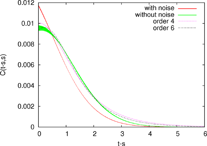
FigureÃÂ 3. Numerical solution of the mean-field equation after 14 iterations in the chaotic case (gÃÂ =ÃÂ 5). We clearly see the numerical instabilities in the no-noise case, which do not exist in the low-noise case.
Modulo this remark, we have first considered the trivial case corresponding to small g values. We took gÃÂ =ÃÂ 0.5 and TÃÂ =ÃÂ 5. We choose as initial process the stationary Ornstein–Uhlenbeck process corresponding to the uncoupled system with ΛÃÂ =ÃÂ 0.1. We drew μα(0) randomly from the uniform distribution in [−1, 1] and vα(0) randomly from the uniform distribution in [0, 1].
Starting from this initial stationary process, we iterated the function 1. Then, during the iterations, we set sαà=à0 in order to match the conditions imposed by Sompolinsky and colleagues. We observe that the method converges toward the expected solution: the mean function converges to 0, while the variance v(t) decreases exponentially fast in time toward a constant value corresponding to the stationary regime. This asymptotic value decreases between two consecutive iterations, which is consistent with the theoretical expectation that v(t)à=à0 in the stationary regime of the trivial case. Finally, we observe that the covariance C(tà−às, s) stabilizes to a curve that does not depend on s and the stationary value (large tà−às) converges to 0.
1. Then, during the iterations, we set sαà=à0 in order to match the conditions imposed by Sompolinsky and colleagues. We observe that the method converges toward the expected solution: the mean function converges to 0, while the variance v(t) decreases exponentially fast in time toward a constant value corresponding to the stationary regime. This asymptotic value decreases between two consecutive iterations, which is consistent with the theoretical expectation that v(t)à=à0 in the stationary regime of the trivial case. Finally, we observe that the covariance C(tà−às, s) stabilizes to a curve that does not depend on s and the stationary value (large tà−às) converges to 0.We applied the same procedure for gà=à5 corresponding to the “chaotic” regime. The behavior was the same for μ(t) but was quite different for the covariance function C(t, s). Indeed, while in theàfirst case the stationary value of v(t) tends to 0 with the number of iterations, in the chaotic case it stabilizes to a finite value. In the same way, the covariance C(tà−às, s) stabilizes to a curve that does not depend on s. The shape of this curve can be extrapolated thanks to Sompolinsky etàal. results. We observe a very good agreement with the theoretical predictions with a fit  corresponding to the fourth expansion of Vq. Using a sixth-order expansion of
  gives a fit
corresponding to the fourth expansion of Vq. Using a sixth-order expansion of gives a fit
where ρ, K, λ are explicit functions of a, b, c, we obtain a slightly better approximation.
Mean-Field Equations for Two Populations with a Negative Feedback Loop
Let us now present a case where the fluctuations of the Gaussian field act on the dynamics of μα(t) in a nontrivial way, with a behavior strongly departing from the naive mean-field picture. We consider two interacting populations where the connectivity weights are Gaussian random variables  for (α, β)à∈ {1, 2}2. We set Sβ(x)à=àtanh(gx) and Iαà=à0, sαà=à0, αà=à1, 2.
for (α, β)à∈ {1, 2}2. We set Sβ(x)à=àtanh(gx) and Iαà=à0, sαà=à0, αà=à1, 2.Theoretical framework
The dynamic mean-field equation for μα(t) is given, in differential form, by:
Let us denote by Gα(μ, v(t)) the function in the righthand side of the equality. Since S is odd,  Therefore, we have Gα(0, v(t))ÃÂ =ÃÂ 0 whatever v(t), and hence the point μ1ÃÂ =ÃÂ 0, μ2ÃÂ =ÃÂ 0 is always a fixed point of this equation.
Therefore, we have Gα(0, v(t))ÃÂ =ÃÂ 0 whatever v(t), and hence the point μ1ÃÂ =ÃÂ 0, μ2ÃÂ =ÃÂ 0 is always a fixed point of this equation.Let us study the stability of this fixed point. To this purpose, we compute the partial derivatives of Gα(μ, v(t)) with respect to μβ for (α, β)ÃÂ ∈ÃÂ {1, 2}2. We have:
and hence at the point μ1ÃÂ =ÃÂ 0, μ2ÃÂ =ÃÂ 0, these derivatives read:
where 
In the case vα(0)à=à0, Jà=à0, sαà=à0, implying vα(t)à=à0, tà≥à0, the equation for μα reduces to:
which is the standard Amari–Cohen–Grossberg–Hopfield system. This corresponds to the naive mean-field approach where Gaussian fluctuations are neglected. In this case the stability of the fixed point μà=à0 is given by the sign of the largest eigenvalue of the Jacobian matrix of the system that reads:
For the sake of simplicity we assume that the two time constants τα are equal and we denote this value τ. The eigenvalues are in this case  where λ are the eigenvalues of
  and have the form:
where λ are the eigenvalues of and have the form:
Hence, they are complex whenever  corresponding to a negative feedback loop between population 1 and 2. Moreover, they have a real part only if
  is nonzero (self interaction).
corresponding to a negative feedback loop between population 1 and 2. Moreover, they have a real part only if is nonzero (self interaction).This opens up the possibility to have an instability of the fixed point (μà=à0) leading to a regime where the average value of the membrane potential oscillates. This occurs if  and if g is larger than:
and if g is larger than:
The corresponding bifurcation is a Hopf bifurcation.
The situation is different if one takes into account the fluctuations of the Gaussian field. Indeed, in this case the stability of the fixed point μà=à0 depends on v(t). More precisely, the real and imaginary part of the eigenvalues of DG(0, v(t)) depend on v(t). Therefore, the variations of v(t) act on the stability and oscillations period of v(t). Though the evolution of μ(t), v(t) are coupled we cannot consider this evolution as a coupled dynamical system, since v(t)à=àC(t, t) is determined by the mean-field equation for C(t, s) which cannot be written as an ordinary differential equation. Note that we cannot assume stationarity here, as in the previous case, since μ(t) depends on time for sufficiently large g. This opens up the possibility of having complex dynamical regimes when g is large.
Numerical experiments
We have considered the case  giving a Hopf bifurcation for gcÃÂ =ÃÂ 2 when JÃÂ =ÃÂ 0 (Figure 4
). The trajectory of μ1(t) and v1(t) is represented in Figure 4
in the case gà=à3. When Jà=à0, μ1(t) presents regular oscillations (with non-linear effects since gà=à3 is larger than the critical value for the Hopf bifurcation, gcà=à2). In this case, the solution v1(t)à=à0 is stable as seen on the figure. When Jà≠à0 the Gaussian field has (small) fluctuations which nevertheless strongly interact with the dynamics of μ1(t), leading to a regime where μ1(t) and v1(t) oscillate periodically.
giving a Hopf bifurcation for gcÃÂ =ÃÂ 2 when JÃÂ =ÃÂ 0 (Figure 4
). The trajectory of μ1(t) and v1(t) is represented in Figure 4
in the case gà=à3. When Jà=à0, μ1(t) presents regular oscillations (with non-linear effects since gà=à3 is larger than the critical value for the Hopf bifurcation, gcà=à2). In this case, the solution v1(t)à=à0 is stable as seen on the figure. When Jà≠à0 the Gaussian field has (small) fluctuations which nevertheless strongly interact with the dynamics of μ1(t), leading to a regime where μ1(t) and v1(t) oscillate periodically.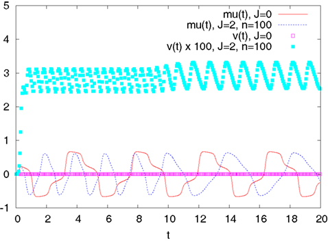
Figureà4. Evolution of the mean õ1(t) and variance 1(t) for the mean-field of population 1, for Jà=à0 and 2, over a time window [0, 20]. n is the number of iterations of 1 defined in Section “Existence and Uniqueness of Solutions in Finite Time”. This corresponds to a number of iterations for which the method has essentially converged (up to some precision). Note that 1(t) has been magnified by a factor of 100. Though Gaussian fluctuations are small, they have a strong influence on μ1(t).
1(t) for the mean-field of population 1, for JÃÂ =ÃÂ 0 and 2, over a time window [0, 20]. n is the number of iterations of 1 defined in Section “Existence and Uniqueness of Solutions in Finite Time”. This corresponds to a number of iterations for which the method has essentially converged (up to some precision). Note that 1(t) has been magnified by a factor of 100. Though Gaussian fluctuations are small, they have a strong influence on μ1(t).The problem of bridging scales is overwhelming in general when studying complex systems and in particular in neuroscience. After many others we looked at this difficult problem from the theoretical and numerical viewpoints, hoping to get closer to its solution from relatively simple and physically/biologically plausible first principles and assumptions. One of our motivations is to better understand such phenomenological neural mass models as that of Jansen and Rit (1995)
.
We consider several populations of neurons and start from a microscopic, i.e., individual, description of the dynamics of the membrane potential of each neuron that contains four terms.
The first one controls the intrinsic dynamics of the neuron. It is linear in this article but this assumption is not essential and could probably be safely removed if needed.
The second term is a stochastic input current, correlated or uncorrelated. The corresponding noise model is very rich, depending on the degree k of smoothness of the g-shapes. It features integrated Brownian noise up to order kÃÂ −ÃÂ 1.
The third term is a deterministic input current, and the fourth one describes the interaction between the neurons through random connectivity coefficients that weigh the contributions of other neurons through a set of functions that are applied to their membranes potentials. The only hypothesis on these functions is that they are smooth and bounded, as well as their first-order derivative. The obvious choice of sigmoids is motivated by standard rate models ideas. Another appealing choice is a smooth approximation to a Dirac delta function thereby opening a window on the world of spiking neurons. Thus, the model presented in this paper is more general than the instantaneous rate model that is underlying Ermentrout’s voltage-based model (Ermentrout, 1998
) even though we have not explored this avenue.
We then derive the mean-field equations and provide a constructive and new proof, under some mild assumptions, of the existence and uniqueness of a solution of these equations over finite and infinite time intervals. The key idea is to look at this mean-field description as a global problem on the probability distribution of the membranes potentials, unlike previous studies. Our proof provides an efficient way of computing this solution and our numerical experiments show a good agreement with previous studies. It is interesting to note that a sufficient condition for the convergence of our algorithm is related to the previously mentioned noise model. We prove that if the noise matrix F is full rank, with bounded eigenvalues, then the algorithm is in general convergent. An important fact to note is that the solutions of the mean-field equations that we construct are fundamentally non-Markovian eliminating the need for such approximations as the introduction of the q parameter summarizing the whole history of the non-Markovian process, see below.
In the case where the nonlinearities are chosen to be sigmoidal our results shed a new light on existing neural mass models. Indeed, as shown in Section “General Derivation of the Mean-Field Equation”, these appear as approximations of the mean-field equations where the intricate but fundamental coupling between the time variations of the mean membrane potentials and their fluctuations, as represented by the covariance functions, is neglected.
An alternative approach has been recently proposed by Chizhov and collaborators
8
(Chizhov and Graham, 2007
; Chizhov et al., 2007
). The approach of these authors consists in reducing the large number, N, of degrees of freedom of the neural assembly by constructing a probability density ρ on the phase space of neurons states in the limit NÃÂ →ÃÂ ∞. This is a non-rigorous approach where the evolution equations for ρ are heuristically derived. Especially, it is assumed that ρ depends on two parameters only: the current time t and the time elapsed since the last spike t*. Under these assumptions the initial phase space of neurons states is mapped to a two dimensional space t, t*, while ρ(t, t*)dt characterizes the fraction of neurons which have fired in the time interval [tÃÂ −ÃÂ t*, tÃÂ −ÃÂ t*ÃÂ +ÃÂ dt]. Therefore, this approach intrinsically holds for integrate and fire neurons models where the neuron’s membrane potential history is summarized by the last spike time, when it is reset to a constant value. As noticed by these authors, this allows to circumvent the main problem in mean-field approaches for firing rate models, that we also discuss in the present paper: When using mean-field theory to characterize stationary regimes, one needs to introduce ad hoc parameters (see e.g., the parameter q introduced in Section “Stationary Solutions”) summarizing the whole history of the non-Markovian process. Introducing a “history cut-off” while resetting the membrane potential to a constant value indeed removes this difficulty. Therefore, it might be interesting to compare our approach in the case of integrate-and-fire models (see above remark on the choice of the nonlinearity), to the approach of Chizhov and collaborators. This could provide some rigorous basis for their analysis and allow to elucidate the role of field fluctuations which does not appear explicitly in the probability density approach.
On more general grounds, our goal is now to extend the present work in several directions.
Bifurcations Analysis of the Dynamic Mean-Field Equations
From the present analysis, and as shown in the simple examples of Section “Numerical Experiments”, the mesoscopic dynamics of the average membrane potential of a neurons population can be really different from the classical phenomenological equations la Jansen–Rit if one includes the non-Markovian fluctuations of the interaction fields, which summarize the cumulative effects of the nonlinear interactions of a given neuron with the bulk of other neurons. Jansen–Rit equations are commonly used in the neuroscience community either to anticipate the dynamics of local field potential in relation with imaging (Optical Imaging, MEGEEG), or to understand neurophysiological disorders such as epilepsy. Bifurcations analysis of these equations reveal dynamical regimes that can be related to experiments (Grimbert and Faugeras, 2006
). They can be generalized using more accurate neural models (Wendling et al., 2005
). Is there any need to generalize these equations, that we claim to be incomplete, while people commonly use them with some satisfaction? Are there new phenomena, experimentally accessible, that can be exhibited by the generalized mean-field equations and that do not appear in the naive ones? These are obviously important questions that we intend to address in the near future. On mathematical grounds, the goal is to make a bifurcation analysis of the map on the space of trajectories, introduced in the present paper. Do any new salient dynamical regimes appear? If such regimes exist, the goal will be, on experimental grounds, to interact with experimentalists in order to see in which conditions such a regime can be exhibited, and what are its implications on cortical columns dynamics or function.
on the space of trajectories, introduced in the present paper. Do any new salient dynamical regimes appear? If such regimes exist, the goal will be, on experimental grounds, to interact with experimentalists in order to see in which conditions such a regime can be exhibited, and what are its implications on cortical columns dynamics or function.Investigations of Nonstationary Regimes
As discussed in this paper, and as is well-known in the physicists’ community (especially spin-glasses community), the dynamic mean-field approach raises serious difficulties as far as one is trying to describe stationary dynamics. On technical grounds, this relies on the non-commutativity of the two limits NÃÂ →ÃÂ ∞ and tÃÂ →ÃÂ ∞ already discussed in Sompolinsky and Zippelius (1982)
. As a result, one is led to introduce ad hoc phenomenological parameters, depending on initial conditions, that can be determined in statistical physics models where the distribution of equilibria is known (Gibbs distribution), using sophisticated techniques such as the replica “trick” (Houghton et al., 1983
). For spin-glasses it is only in the high temperature regime that a simple solution to this problem is known. This restriction also appears in the present paper, where the existence and uniqueness of a stationary solution is proved only for low values of the gain parameter g (which plays a role similar to the inverse temperature). However, we are not so much interested in stationary dynamics, since brain processes are ultimately nonstationary. Our approach, valid for any finite timeÃÂ T, opens up the possibility to characterize mean-field equations in transient regimes, with an analysis strategy that can moreover be easily implemented. To the best of our knowledge, this type of techniques has never been used in the statistical physics community, where iterations on space trajectories are not in the standard toolbox. Therefore, our work could allow the (numerical) investigation of cortical columns submitted to nonstationary inputs, with strong implications on neuroscience.
Extension to A Larger Class of Models
A very challenging question is the application of this theory to spiking neurons models. We have briefly mentioned in Section “Discussion” that this may be possible through the use of non-sigmoidal functions in the interaction terms. This idea could be applied to the analysis of Integrate and Fire models with conductance based synapses, which constitute good models of spiking neurons. As discussed at the end of Section “Discussion”, the analysis of the mean-field equations could be simplified by the fact that memory is reset after a neuron fires. There is however a need to characterize parameter space regions where neurons can take an arbitrary large time to fire for the first time (Cessac, 2008
; Cessac and Viéville, 2008
). This is the main obstruction in the application of our theory to this type of models.
A. Identification of the Mean-Field Equations
Ben-Arous and Guionnet studied from a mathematical point of view the problem of finding a mean-field description of large networks of spin-glasses. They obtained using different methods of stochastic analysis a weak limit of the law of a given spin and proved their independence.
Our equations do not directly fit in their study: indeed, the spin intrinsic dynamics is nonlinear while the interaction is linear, and everything in done in dimension one. Nevertheless, their proof extends to our case which is somehow more simple. For instance in the case of the Simple Model with one population, we can readily adapt their proof in our case. More precisely, let PÃÂ =ÃÂ 1, the equation of the network reads:
In this case, we define for  the effective interaction term
  which is the effective interaction process defined in Section “The Mean-Field Equations”, i.e., the Gaussian process of mean
  and of covariance:
the effective interaction term which is the effective interaction process defined in Section “The Mean-Field Equations”, i.e., the Gaussian process of mean and of covariance: Let us note  the law of the membrane potential when there is no interaction (it is an Ornstein–Uhlenbeck process), and the empirical measure
  We can prove that under theÃÂ probability distribution averaged over the connectivities, see below, the empirical measure satisfies a large deviation principle with good rate function H defined as in Guionnet (1997)
. Using this large deviation result, we can prove annealed and quenched tightness of the empirical measure, and finally its convergence toward the unique process where the good rate function H achieves its unique minimum, which is defined by the property of having a density with respect to and whose density satisfies the implicit equation:
We can prove that under theÃÂ probability distribution averaged over the connectivities, see below, the empirical measure satisfies a large deviation principle with good rate function H defined as in Guionnet (1997)
. Using this large deviation result, we can prove annealed and quenched tightness of the empirical measure, and finally its convergence toward the unique process where the good rate function H achieves its unique minimum, which is defined by the property of having a density with respect to and whose density satisfies the implicit equation:
the law of the membrane potential when there is no interaction (it is an Ornstein–Uhlenbeck process), and the empirical measure We can prove that under theÃÂ probability distribution averaged over the connectivities, see below, the empirical measure satisfies a large deviation principle with good rate function H defined as in Guionnet (1997)
. Using this large deviation result, we can prove annealed and quenched tightness of the empirical measure, and finally its convergence toward the unique process where the good rate function H achieves its unique minimum, which is defined by the property of having a density with respect to and whose density satisfies the implicit equation:
where ε denotes the expectation over the effective interaction process UQ.
We can also prove following the steps of Ben-Arous and Guionnet (1997)
that there exists a unique solution to this equation, and that this solution satisfies the nonlinear non-Markovian stochastic differential equation:
which can also be written as our mean-field equation, averaged on the connectivities (see Ben-Arous and Guionnet, 1995
). More precisely, let LV be the law of the solution of the equation:
which is exactly Eq.ÃÂ 33. They prove that V satisfies the nonlinear equation:

This result is probably extendable to the multi-population case using the multidimensional Girsanov’s theorem, but the corresponding mathematical developments are out of the scope of this paper.
B. The Resolvent
In this appendix we introduce and give some useful properties of the resolvent ΦL of a homogeneous differential equation:

where  .
.
.Definition B.1. The resolvent of Eq.ÃÂ 61 is defined as the unique solution of the linear equation:
where IdP is the Pà×àP identity matrix.
Proposition B.1. The resolvent satisfies the following properties:
(i) ΦL(tà+às, t0)à=àΦL(tà+às, t)à÷àΦL(t, t0)
(ii) ΦL(t, t0) is invertible of inverse ΦL(t0, t) which satisfies:
(iii) Let ‖ ‖ be a norm on  Pà×àP and assume that
  on [t0,àT]. Then we have:
on [t0,ÃÂ T]. Then we have:
Pà×àP and assume that on [t0,àT]. Then we have:
Similarly, if  on [t0, T] we have:
on [t0, T] we have:
(iv) We have
Proof. The properties (i) and (ii) are directly linked with the property of group of the flow of a reversible ODE. (iii) is an application of Grunwald’s lemma. (iv) is obtained by a first-order Taylor series expansion.
Theorem B.2 (Solution of an inhomogeneous linear SDE). The solution of the inhomogeneous linear stochastic differential equation:
can be written using the resolvent:
Proof. Pathwise (strong) uniqueness of solution directly comes from the results on the SDE with Lipschitz coefficients (see e.g., Karatzas and Shreve, 1991
, Theorem 2.5 of Chapter 5). It is clear that Xt0ÃÂ =ÃÂ X0. We use Itô’s formula for the product of two stochastic processes to prove that the process Eq.ÃÂ 67 is solution of Eq.ÃÂ 66:
Hence the theorem is proved.
C. Matrix Norms
In this section we recall some definitions on matrix and vector norms. Let n ×àn be the set of nà×àn real matrices. It is a vector space of dimension n2 and the usual Lp norms 1à≤àpà≤à∞ can be defined. Given Là∈àn ×àn, we note  the corresponding norm. Given a vector norm, noted ‖ ‖, on n the induced norm, noted ‖ ‖, on n ×àn is defined as
n ×àn be the set of nà×àn real matrices. It is a vector space of dimension n2 and the usual Lp norms 1à≤àpà≤à∞ can be defined. Given Là∈àn ×àn, we note the corresponding norm. Given a vector norm, noted ‖ ‖, on n the induced norm, noted ‖ ‖, on n ×àn is defined as
Since n×n is finite dimensional all norms are equivalent. In this article we use the following norms
n×n is finite dimensional all norms are equivalent. In this article we use the following norms(i) 
(ii) 
(iii)  This so-called spectral norm is equal to the square root of the largest singular value of L which isÃÂ the largest eigenvalue of the positive matrix LTL. If L is positive definite this is its largest eigenvalue which is also called its spectral radius, noted ρ(L).
This so-called spectral norm is equal to the square root of the largest singular value of L which isÃÂ the largest eigenvalue of the positive matrix LTL. If L is positive definite this is its largest eigenvalue which is also called its spectral radius, noted ρ(L).D. Important Constants
Table 1
summarizes some notations which are introduced in the article and used in several places.
E. Proof of Lemma 2
Lemma E.1. The following upperbounds are valid for all nà≥à1 and all s, tà∈à[t0, T].

where μ and σmax are defined in Lemma 1,  is defined in Assumption 1.
is defined in Assumption 1.Proof. The first inequality follows from taking the infinite norm of both sides of Eq.ÃÂ 41 and using Assumption (a) in 1 and Eq.ÃÂ 64, Lemma 1, and Assumption (c) in 1.
The second inequality follows from taking the infinite norm of both sides of Eq.ÃÂ 42 and using Assumption (a) in 1 and Eqs.ÃÂ 64 andÃÂ 65, Lemma 1, and Assumption (b) in 1.
F. Proof of Lemma 3
Lemma F.1. For all tà∈à[t0, T] all αà=à1,…,kP, and nà≥à1, we have
where λmin is the smallest singular value of the symmetric positive definite matrix ΦL(t, t0)ΦL(t, t0)T for tÃÂ ∈ÃÂ [t0, T] and  is the smallest eigenvalue of the symmetric positive definite covariance matrix
is the smallest eigenvalue of the symmetric positive definite covariance matrix Proof.  is larger than
  which is larger than the smallest eigenvalue of the matrix
  This smallest eigenvalue is equal to
is larger than which is larger than the smallest eigenvalue of the matrix This smallest eigenvalue is equal to
In the last expression the first term is larger than the smallest eigenvalue  of the matrix
  which is positive definite since we have assumed the Gaussian random variable Z0 nondegenerate. The second term is equal to the smallest singular value
  of the matrix
  which is also strictly positive since
  is invertible for all tÃÂ ∈ÃÂ [t0, T], see Appendix B.
of the matrix which is positive definite since we have assumed the Gaussian random variable Z0 nondegenerate. The second term is equal to the smallest singular value of the matrix which is also strictly positive since is invertible for all tÃÂ ∈ÃÂ [t0, T], see Appendix B.G. Proof of Lemma 4
Lemma G.1. For all αà=à1,…,kP and nà≥à1 the quantity  is lowerbounded by the positive symmetric function:
is lowerbounded by the positive symmetric function:
where  is the strictly positive lower bound, introduced in 3.1, on the singular values of the matrix F(u) for uÃÂ ∈ÃÂ [t0, T].
is the strictly positive lower bound, introduced in 3.1, on the singular values of the matrix F(u) for uÃÂ ∈ÃÂ [t0, T].Proof. We use Eq.ÃÂ 42 which we rewrite as follows, using the group property of the resolvent ΦL:
We now assume sÃÂ <ÃÂ t and introduce the following notations:
Let eα, αà=à1,…,kP, be the unit vector of the canonical basis whose coordinates are all equal to 0 except the αth one which is equal to 1. We note Eα(t) the vector  We have, dropping the index n for simplicity:
We have, dropping the index n for simplicity:
Note that the last expression does not depend on s, since A(s)ÃÂ +ÃÂ B(s, t)ÃÂ =ÃÂ A(t), which is consistent with the first equality. The reason why we introduce s in this expression is to simplify the following calculations.
The expression  is the sum of four sub-expressions:
is the sum of four sub-expressions:
which is ≥0 because A(s) is a covariance matrix,
which is also ≥0 because a(t, s) is a covariance matrix function,
Because a(t, s) is a covariance matrix function, we have

and, as seen above,  Because
  we also have
Because we also have
and, as it can be readily verified, this implies 
Therefore, we can lowerbound  by the fourth subexpression:
by the fourth subexpression:
since B(s, t) and a(s, s) are covariance matrixes. We next have
by definition of  Therefore
Therefore
where  is the smallest eigenvalue of the symmetric positive matrix C. Similarly we have
is the smallest eigenvalue of the symmetric positive matrix C. Similarly we have
Let us write γ(u)ÃÂ =ÃÂ F(u)F(u)T. We have (Assumption 1):
Combining these results, we have

H. Proof of Lemma 5
Lemma H.1. The 2n-dimensional integral
where the functions ρi(ui, vi), iÃÂ =ÃÂ 1,…,n are either equal to 1 or to  (the function θ is defined in Lemma 4), is upperbounded by kn/(nÃÂ −ÃÂ 1)! for some positive constant k.
(the function θ is defined in Lemma 4), is upperbounded by kn/(nÃÂ −ÃÂ 1)! for some positive constant k.Proof. First note that the integral is well-defined because of Lemma 4. Second, note that there exists a constant K such that
 for all (u, v)ÃÂ ∈ÃÂ [t0, t ÃÂ s]2,
i.e.,  . Therefore the integral is upperbounded by
  where K0ÃÂ =ÃÂ max(1, K) times the integral obtained when
  for all iÃÂ =ÃÂ 1,…,n. Let us then consider this situation. Without loss of generality we assume t0ÃÂ =ÃÂ 0. The cases nÃÂ =ÃÂ 1, 2, 3 allow one to understand the process.
. Therefore the integral is upperbounded by where K0ÃÂ =ÃÂ max(1, K) times the integral obtained when for all iÃÂ =ÃÂ 1,…,n. Let us then consider this situation. Without loss of generality we assume t0ÃÂ =ÃÂ 0. The cases nÃÂ =ÃÂ 1, 2, 3 allow one to understand the process.
Let us rotate the axes by  by performing the change of variables
by performing the change of variables
Using the symmetry of the integrand in s and t and the change of variable, the integral in the righthand side of Eq.ÃÂ 68 is equal to (see Figure 5
):
FigureÃÂ 5. The change of coordinates.
where  and
and 
and Let us now look at I2. It is upperbounded by the factor  times the integral
times the integral
Since in the area of integration  we are led to the product of 2/5 by the one-dimensional integral
we are led to the product of 2/5 by the one-dimensional integral
where 
Similarly I3 is upperbounded by the product of  times the integral
times the integral
where  One easily shows then that:
One easily shows then that:
It can be verified by using a system for symbolic computation that 0à<àαià<à1 for all ià≥à1. One also notices that
therefore
and this finishes the proof.
The authors declare that the research was conducted in the absence of any commercial or financial relationships that could be construed as a potential conflict of interest.
This research was partly supported by funding of the European Union under the grant no. 15879 (FACETS) and the Fondation d’Entreprise EADS. It was also supported by the MACACC ARC INRIA and the Doeblin CNRS Federation.
- ^ When we come to the mean-field equations they will be modeled as random variables.
- ^ We have modified the original model which is not voltage-based.
- ^ We note Γ(t) the matrix F(t)F(t)T.
- ^ In Bogachev (1998 ; Chapter 3.8), the property is stated whenever the mean and covariance are defined on a separable Hilbert space.
- ^
For simplicity we abuse notations and identify
 and X.
 - ^
The notation
 is introduced in Appendix C.
 - ^ More precisely, this is the only minimum for the large deviation functional.
- ^ We thank one of the referees for pointing out these references to us.