Irregular persistent activity induced by synaptic excitatory feedback

Introduction

The mechanisms of working memory at the neuronal level have been investigated in the last three decades using single neuron electrophysiological recordings in monkeys performing delayed response tasks (Funahashi et al., 1989 ; Fuster and Alexander, 1971 ; Fuster and Jervey, 1981 ; Goldman-Rakic, 1995 ; Miyashita, 1988 ). These tasks share in common a ‘delay period’ during which the monkey has to maintain in working memory information needed to solve the task after the end of the delay period. One of the major findings of these experiments is that neurons in many areas of association cortex exhibit selective ‘persistent activity’ during the delay period—they increase (or decrease in some cases) their firing rates compared to the baseline period, selectively for one or several cues whose identity is needed for the monkey to perform the task correctly after the end of the delay period. This has led to the hypothesis that persistent activity of neurons in such areas is what allows the monkey to maintain the identity of a stimulus in working memory. In particular, neuronal persistent activity in prefrontal cortex (PFC) has all the properties expected for a working memory system: it is maintained until the end of the delay period, even when the duration of this delay period is changed from trial to trial (Funahashi et al., 1989 ; Nakamura and Kubota, 1995 ); the monkey makes an error when persistent activity stops before the end of the trial (Funahashi et al., 1989 ).

Most experimental papers reporting persistent activity have focused purely on changes in firing rates of the recorded neurons. Several recent studies have investigated in more detail the statistics of firing of neurons in dorsolateral PFC during such tasks (Compte et al., 2003 ; Shinomoto et al., 1999 ). In particular, Compte et al. (2003) found that neurons fire in a highly irregular fashion in all periods of the task. The average CV is close to one in the baseline period, and is higher than 1 in the delay period, both for preferred and non-preferred stimuli.

Most models of working memory in recurrent neuronal circuits (reviewed in Brunel, 2004 ) generate persistent activity due to excitatory feedback loops in such circuits. These models are able to account for the firing rates observed in such tasks (Amit and Brunel, 1997 ; Brunel, 2000 ; Brunel and Wang, 2001 ), though not very robustly. However, these models do not account for the high irregularity shown in the experiments. While high irregularity can be obtained robustly in the baseline period, provided inhibition is sufficiently strong, because neurons receive synaptic inputs that are subthreshold in average and firing is due to temporal fluctuations in these inputs (Amit and Brunel, 1997 ; van Vreeswijk and Sompolinsky, 1996 , 1998 ), persistent activity states typically involve neurons which receive supra-threshold inputs (Brunel, 2000 ) and therefore exhibit much more regular firing. This has led to alternate models that propose different mechanisms for working memory maintenance, that rely on an increase of inhibition in the persistent state compared to the background state (Renart, 2000 ; Renart et al., 2007 ).

In this paper, we re-examine the issue of irregularity in recurrent networks in which multistability is induced by recurrent excitation. We show that recurrent excitation can lead to persistent activity that is more irregular than background activity, provided two conditions are fulfilled: (i) post-spike reset is close to threshold (i.e. neurons do not have a pronounced hyperpolarization following a spike, Troyer and Miller, 1997 ) and (ii) saturation of post-synaptic currents at high pre-synaptic firing rates, which is implemented by short-term depression (Tsodyks and Markram, 1997 ).

Materials and Methods

The model

We consider a fully connected network of N excitatory integrate-and-fire neurons. Each neuron has two sources of input currents: an external current, I_i,ext and the recurrent current I_i,rec due to the spikes arriving from all other neurons in the network. The membrane potential V_i of neuron i (i =  1, … , N) evolves in the sub-threshold range according to:

where τ is the integration time constant of the membrane and the currents are expressed in units of the potential. If at time t the voltage reaches the thresholdθ, a spike is emitted and the voltage is reset to a value V_r for an interval (t, t+τ _rp) where τ_rp is the refractory period.

The external input is assumed to be Gaussian and δ-correlated:

where μ_ext is a constant input, σ_ext measures the fluctuations around μ_ext and η_it) is white noise uncorrelated from neuron to neuron: ⟨η_i(t)⟩  =  0, ⟨η _i(t)η _j(t′) ⟩  =  δ_ijδ(t-t^′).

Spikes arriving at synapses from excitatory neurons produce a fast component that models AMPA receptor-mediated currents, and a slow-decaying component, mimicking NMDA receptor-mediated currents. Since the network is fully connected, all neurons receive the same recurrent synaptic input,

where s(t) and z(t) denote respectively the fast and slow components of the synaptic current which obey to:

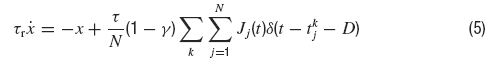
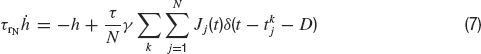
where τ_r is the rise time, τ_d the decay time constant of the post-synaptic AMPA current, x(t) is an auxilliary variable and D the synaptic delay. The fraction of charge mediated by the NMDA-like component is denoted by γ and τ_rN, τ_dN are respectively the rise and decay time of the NMDA post-synaptic current. Individual synaptic strengths scale as 1∕N, see the factor in front of the sums in Equations (5, 7).

The time dependence of the synaptic efficacy J_j(t) is due to the presence of short-term depression (STD). We use the phenomenological model introduced by Tsodyks and Markram, (1997) . The synaptic transmission is described in terms of fraction of available resources, y_j(t)∈ [0,1], where the index j refers to pre-synaptic neuron. Upon arrival of a spike, a fraction u of currently available resources is activated, becoming temporarily unavailable. In between spikes, available resources recover exponentially with a time constant τ_rec, i.e.

The current produced is proportional to the instantaneous fraction of activated synaptic resources at the presynaptic emission time. Hence, J(t) is given by:

where J is the maximal efficacy.

Analytical methods

The model is studied using both numerical simulations and analytical techniques. Analytical calculations are performed using a ‘mean-field’ approach, following previous studies (Amit and Tsodyks, 1991 ; Amit and Brunel, 1997 ; Romani et al., 2006 ).

Statistics of input currents in the large N limit. Since the strength of the synaptic efficacies is O(1∕N), the fluctuations in the recurrent currents are and hence they can be neglected in the limit N →∞. In this limit the fluctuations in the inputs are induced by external inputs exclusively and are thus independent from neuron to neuron. Equations (4, 5, 6, 7) become:

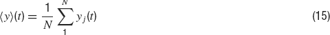
where is the instantaneous population-averaged synaptic efficacy, and ν(t) is the instantaneous population-averaged firing rate. The average synaptic efficacy is a function of the first moment of the ditribution of the available resources in the presynaptic population:

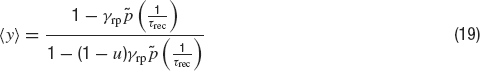
where ⟨y⟩(t) is given by:

In an asynchronous state in which ν(t) = ν, the synaptic inputs are therefore

Hence, the computation of the recurrent synaptic currents requires the knowledge of the average emission rate ν and of the average fraction of the available resources ⟨y⟩, which depends itself on the statistics of firing of the network. Note again that since the fluctuations of the recurrent part of the synaptic input vanish and the external current is gaussian and δ- correlated, the fluctuating parts of the synaptic input to different neurons are uncorrelated.

Average firing rate. In the presence of white noise, the average emission rate, ν, defined as the inverse of the average first passage time, is given by the well-known formula (Ricciardi, 1977 ):

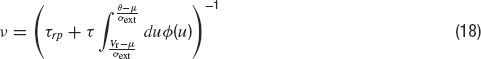
where μ is given by Equation (17), and .

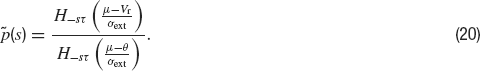
Average fraction of available resources. The expression of the average fraction of the available resources in a network of LIF neurons has been computed recently (Romani et al., 2006 ). The first moment of the distribution of available synaptic resources is

where is the Laplace transform of the distribution of presynaptic ISIs and . The Laplace transform of an Ornstein-Uhlenbeck process was derived in Alili et al. (2005) in terms of Hermite functions H_l(z)

To summarize, the average firing rate in asynchronous states of the network is given by the solutions of equations:

The coefficient of variation of the ISIs—the standard deviation of the ISI divided by the mean ISI—is given by the following expression:

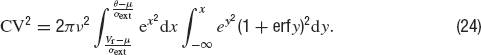
where μ is given by Equation (22).

These equations are integrated numerically to obtain the dependence of the rate ν and CV on mean inputs μ or synaptic strength J.

Numerical methods

The equations for the membrane potential V_i(t) (Equation (1) plus condition for spike emission and refractoriness) with the recurrent current I_rec (Equations 3, 4, 5, 6), external current I_ext (Equation 2) and for the fraction of available resources at each synapse (Equation 8) are integrated using a Runge-Kutta method with gaussian white noise with a time step Δ t (Honeycutt, 1992 ). The mean value of the external current μ_ext is calculated using mean-field equations such that the background activity is at a choosen value ν_sp, i.e.

The network has been simulated using the following protocol. The simulation starts by a pre-stimulus interval of 1 second, during which the network receives no external stimulation. Then a stimulus is presented during 500 ms. Stimulus presentation consists in increasing the value of the external mean synaptic input by a contrast factor λ. Last, a delay period of several seconds follows in which the external stimulus is removed. Delay period activity and CV are estimated excluding the first second following the stimulus presentation, to ensure the network has reached its steady state. The parameters used in the simulations are summarized in Table 1 , except when stated otherwise.

TABLE 1

Table 1. Paramoters used in the simulations of a network of N excitatory cells connected by synapses with STD.

Spatial working memory model

We also simulated a network model with a spatial structure (Camperi and Wang, 1998 ; Compte et al., 2000 ; Renart et al., 2003 ). The network is composed of N_E pyramidal cells and N_I interneurons, with N_E =  4 N_I. Excitatory neurons are selective to an angular variable θ∈ [0,2π]. Neuron i (i =  1,… ,N_E) has preferred angle θ_i =  (2π i)∕ N_E. Hence, neurons of the network cover uniformly all the angles along a circle. Both excitatory and inhibitory cells are modelled as leaky integrate-and-fire neurons whose parameters are summarized in Tables 1 and 2 . Both types of neurons receive non-selective external inputs, modelled as external currents of mean and and SD and as in Equation (2). Neurons receive their recurrent excitatory inputs through AMPAR- and NMDAR-mediated transmission and their inhibitory inputs through GABAR-mediated currents. These currents are modelled as in ‘The Model’ with time constants summarized in Tables 1 (AMPA and NMDA) and 2 (GABA). Only excitatory-to-excitatory connections are endowed with STD. In contrast to the network used until now (a homogeneous network with no spatial structure), the excitatory-to-excitatory recurrent connections between neurons depend on the difference between their preferred cues. This is implemented taking the absolute synaptic efficacy between neuron i and neuron j to be J_ij =  J(θ _i− θ_j), where J(θ _i− θ_j) is given by

In this equation, J⁻ represents the strength of the weak crossdirectional connections, J⁺ the strength of the stronger isodirectional connections and σ_J is the width of the connectivity footprint, J(θ _i− θ_j). The normalization condition:

imposes a relationship between J⁺, J⁻ and σ_J; therefore the only remaining free parameters are J⁺ and σ_J, while J⁻ is determined by Equation (27). This normalization condition is used in order to maintain a fixed background activity as J⁺ is varied (Amit and Brunel, 1997 ; Compte et al., 2000 ).

TABLE 2

Table 2. Parameters used in the simulations of a network with spatially structured connectivity. Other paramenters as in Table 1.

Other connections (inhibitory-to-excitatory, excitatory-to-inhibitory and inhibitory-to-inhibitory) are unstructured, i.e. they are independent on the preferred angle of both neurons. In order to achieve the desired levels of background activity of the excitatory and inhibitory population, the mean, and , of the external inputs have been chosen using mean-field equations:

where J_IE is chosen equal to J_EE, while inhibitory connections are chosen to be stronger than the excitatory ones by a factorα, so that J_EI =  J_II =  α J_EE. The simulation protocol is similar to the one used until now, but the cue presentation is modelled enhancing by a factor λ the value of the mean external input to pyramidal cells whose preferred cues are close to the stimulus (θ∈[θ _s−18^°, θ_s+18^°]).

Results

f-I and CV-I curves of IF neurons with low reset

We first consider how the firing rate and CV of the integrate-and-fire neuron depend on its mean synaptic inputs. This is done by plotting the f-I curve (frequency as a function of mean input) and CV-I curve (CV as a function of mean input). The qualitative features of these curves are crucial to understand the solutions of mean-field equations that give the collective properties of the network, as we will see below. The firing frequency is represented as a function of the mean synaptic input in Figure 1 A for a low value of the reset potential (V_r =  10 mV). It shows two regimes: for mean synaptic inputs well below threshold, firing is driven by the fluctuations around the mean input. In this region, the f-I curve is convex. For mean synaptic inputs well above threshold, the neuron is in a supra-threshold firing mode. Firing is essentially driven by the mean synaptic input, the firing frequency is relatively independent of the fluctuations and the f-I curve is concave. The inflexion point is close to the point at which the mean synaptic input is equal to the firing threshold.

FIGURE 1

Figure 1. f—I curve and CV—I curve of a LIF neuron with low reset. (A) f—I curve of the LIF neuron. Output frequency, Equation (18), as a function of the mean input, for θ  =  20 mV, σ_ext =  5 mV, τ_rp =  5 ms, τ_m =  20 ms and V_r =  10 mV. (B) Coefficient of variation, Equation (24) as a function of the mean current input for the same parameters.

How the CV behaves as a function of the mean synaptic input is shown in Figure 1 B: for very small inputs (those corresponding to low rates) the CV is almost 1, since firing is due to rare fluctuations that bring the neuron to threshold (Poisson-like firing). As the mean input increases, firing becomes more and more regular, and the CV starts to decrease significantly when the mean inputs are close to threshold. In the supra-threshold regime the CV becomes small, since the inter-spike interval density becomes peaked around the mean time for the neuron to cross threshold. The CV tends to zero as the mean inputs become large.

Persistent activity of excitatory networks of IF neurons with low reset and linear synapses

We now turn to an investigation of the dynamics of the network in absence of short-term depression, which is obtained in the limit u → 1, τ_rec→ 0. In this limit the relationship between the presynaptic firing rate and the average post-synaptic currents becomes linear. As described in Brunel (2000) , the firing rates ν in background and persistent activity states can be obtained as the solutions of the equation:

where in the first argument of the function Φ, we have rewritten the mean input μ as the sum of its value μ_sp in the background state, plus the deviation from this value when the population has an average firing rate ν. This second term in the mean currents is proportional to J, the total synaptic efficacy, and to ν−ν _sp. The solutions of Equation (30) are the intersections of the response function ν  =  Φ (μ, σ_ext) and the straight line ν  =  ν _sp+(μ−μ _sp)∕ τJ in the μ- ν plane. For low values of the synaptic efficacy J, there is a unique solution which corresponds to the background state ν_sp. When increasing the strength of the synaptic efficacy J, the slope of the straight line decreases. At a critical value of J, the straight line becomes tangent to the transfer function. This intersection represents the onset of working memory. Note that at this intersection point the response function is necessarily concave.

As shown in Figure 2 A, as J increases further, Equation (30) develops two other solutions: the highest one ν  =  ν _per represents the persistent activity state and is potentially stable; the lowest one, ν  =  ν ^* is unstable and represents the boundary of the basins of attraction of persistent and background states. The values of the coefficient of variation relative to these three solutions are shown in Figure 2 B. The CV of the background activity state is near 1, while the persistent activity state is in the region in which the CV is small. This is not surprising because, as mentioned above, the onset of working memory happens at the point at which the straight line is tangent to the f-I curve and at this point the response function is necessarily concave. Thus, the persistent activity state is in the supra-threshold region for any value of the synaptic strength.

FIGURE 2

Figure 2. Single cell and network properties with low reset and linear synapses. Parameters: θ  =  20 mV, σ_ext =  5 mV, τ_rp =  5 ms, τ_m =  20 ms and V_r =  10 mV. (A) f—I curve (firing rate of a single LIF neuron as a function of mean input). The intersections between the f—I curve (thick line) of the LIF neuron and the straight line (thin line) correspond to solutions of Equation (30), shown by diamonds, for J =  18 mV. The three solutions correspond to the background activity state (stable), the limit of the basin of attraction (unstable) and the persistent activity state (stable). (B) CV—I curve (CV of a single LIF neuron as a function of mean input). Diamonds: Values of the CV for the three states shown in A. (C): Bifurcation diagram showing firing rate of the excitatory network as a function of synaptic strength J. The background activity corresponds to the red horizontal curve (lowest branch), the dotted curve (intermediate branch) is the boundary of the basin of attraction and the black curve (highest branch) represents the evolution of the persistent activity. (D) Bifurcation diagram showing how the CV depends on J: the persistent activity (black curve, lowest branch) has a CV which is well below the CV of the background activity (highest branch, red curve) for all values of J.

Figure 2 C shows the bifurcation diagram—how the solutions of Equation (30) depend on J. The lowest horizontal branch corresponds to the background solution, the intermediate branch to the unstable solution and the upper branch to the persistent activity state. As can be seen in Figure 2 D, the CV of the persistent activity state is always lower than the CV of the background activity state (upper horizontal branch)— in fact it is around 0.4 at the bifurcation point and goes to zero as the synaptic strength increases.

This highly regular firing predicted by the mean-field calculations during persistent activity is confirmed by numerical simulations; Figures 3 A and 3 B represent respectively the spike trains of 10 neurons and the evolution of the mean firing rates during time for a fixed value of the synaptic efficacy. In the pre-stimulus interval (0–1000 ms) the network is in the background state and the CV is close to one (C =  0.89), while during the delay period (1500–2500 ms) we found persistent activity with small CV (CV =  0.23). Figures 3 C and 3 D compare mean-field predictions and simulations for both rates and CVs.

FIGURE 3

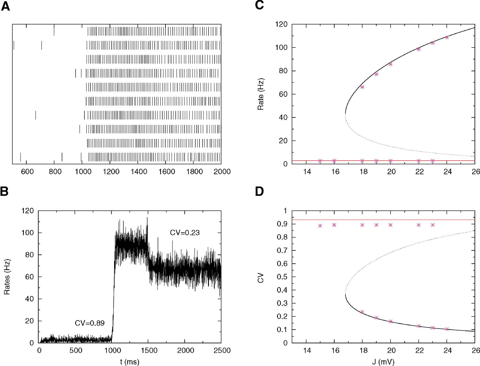
Figure 3. Simulations versus theory. The network is submitted to the following protocol: pre-stimulus interval (0–1000 ms); Stimulus presentation (1000–1500 ms); and delay activity (1500–2500 ms). The total excitatory coupling strength is J =  18 mV. The external current is chosen in order to have a background activity of 3 Hz. Other parameters as in Figure 2 . (A) Spike trains of 10 neurons in the interval 500–2000 ms. (B) Average instantaneous firing rate as a function of time (in bins of 1 ms); the mean value of the CV in the background and persistent activity are indicated in the graph. (C) Bifurcation diagram showing firing rate versus J: Mean-field (solid lines) versus simulations (symbols). (D): Bifurcation diagram showing CV versus J: Mean-field (solid lines) versus simulations (symbols).

Effect of reset and membrane time constant on CV—I curve

In the previous section we described the behaviour of a network model in which the synapses are a linear function of the output frequency and in which the value of the reset potential is relatively far from threshold (θ −V_r =  10 mV). We now turn to the analysis of the effect of increasing the value of the reset potential (Troyer and Miller, 1997 ), keeping a linear description of the synaptic efficacies.

Figure 4 shows the effect of increasing V_r on the firing rate and on the CV. Increasing V_r increases the gain of the f—I curve, since the neuron is closer to threshold just after a spike has been emitted. The effect on the CV is more interesting: when V_r is large enough (V_r =  15 mV in Figure 4 ), the CV—I curve becomes non-monotonic—it first increases when the mean input increases, reaches a maximum at a value which is smaller than V_r, and then decreases monotonically as the mean inputs go towards the supra-threshold range. Hence, there is a large region of mean inputs for which the CV is larger than one. The reason for a maximum in CV for mean inputs smaller than the reset is that in these conditions, the instantaneous firing probability is higher just after firing that it is afterwards; hence, there is a higher probability of short interspike intervals, compared to a Poisson process with the same rate. Therefore, the CV is larger than one. This effect can also be seen by plotting the CV as a function of rate, while the CV becomes 1 at low enough rates for any value of V_r, the range in which the CV is larger than 1 depends in a pronounced way on how close V_r is to the threshold (see Figure 4 B).

FIGURE 4

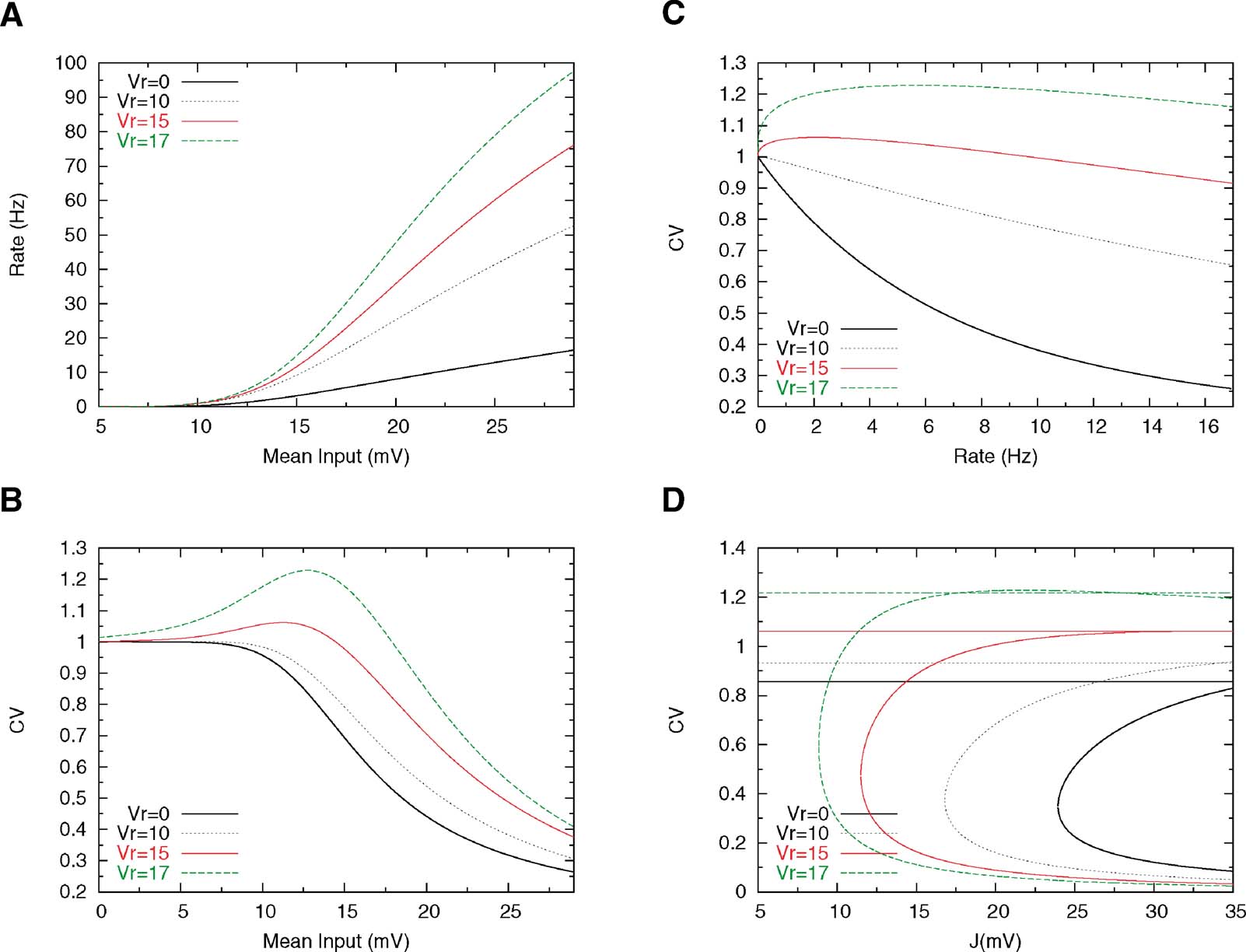
Figure 4. Effect of reset potential on single cell and network behaviour. Other parameters are Θ  =  20 mV, τ_m =  20 ms, τ_rp =  5 and σ_ext =  5 mV. (A) f—I curves for four different values of the reset potential, indicated on the graph; the steepness of the f-I curve increases with increasing V_r. (B) The CV-I curve develops a peak when V_r is large enough. (C) CV as a function of the mean firing rate. (D) Bifurcation diagrams for different values of V_r; the values of the CV in persistent activity close to the bifurcation increase with V_r, but the gap between persistent and background CVs remain large (∼ 0.5) at any value of the CV.

Changing the membrane time constant has also a pronounced effect on rate and CV. Decreasing the membrane time constant increases the steepness of the f—I curve, as shown in Figure 5 A, since shorter integration time leads to shorter ISIs, which means higher firing rates. Furthermore, reducing the membrane time constant has the effect of shortening the transients of the voltage, which leads to a decrease in the size of the peak in the CV—I curve for low values of τ (see Figure 5 B); this happens since, as mentioned above, the transient dynamics just after the spike is responsible for the increase in the probability of firing at short ISIs. However, this effect is not very pronounced and, as we can see in Figure 5 C, decreasing τ yields a flattening of the CV versus rate curve, leading to high CV values for a very broad range of firing rates.

FIGURE 5

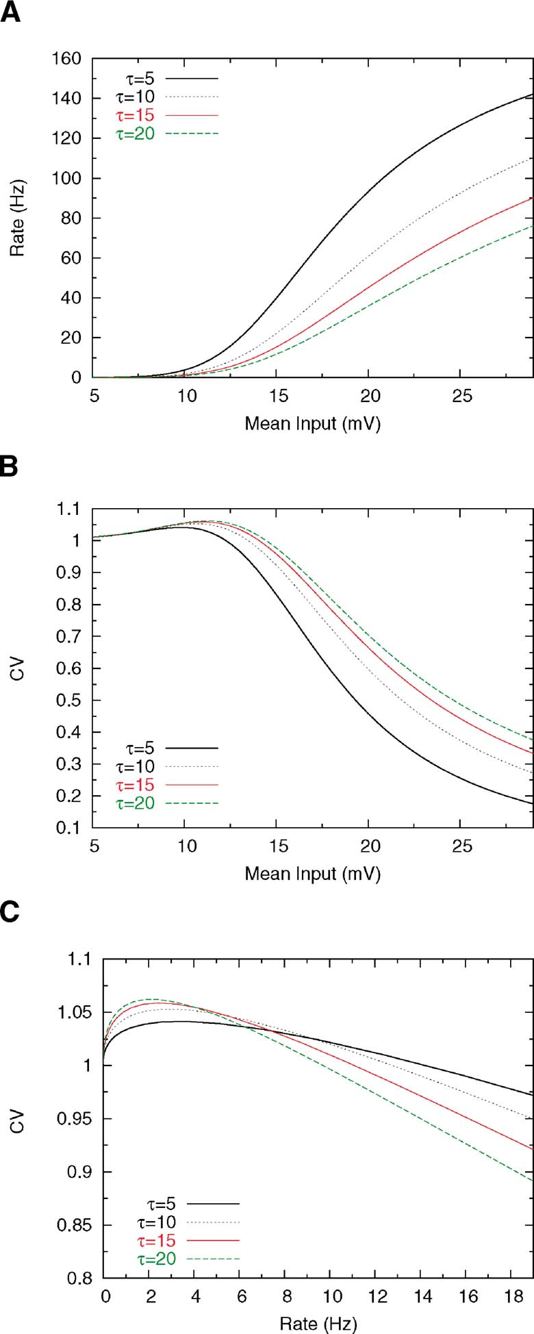
Figure 5. Effect of membrane time constant on rate and CV. Others parameters are Θ  =  20 mV, V_r =  15 ms, τ_rp =  5 and σ_ext =  5 mV. (A) f—I curve for several values ofτ. (B) CV—I curve. (C) CV as a function of mean firing rate.

Can this increase in V_r in itself solve the problem of the irregularity of persistent activity? Figure 4 D shows that while increasing V_r does increase the CV of both background and persistent activity states, the large gap between the CV in the background state and the one in the persistent state persists. This is due to the fact that the high-CV region remains confined to the subthreshold range, while we have seen in the last section that with linear synapses, the persistent activity state is necessarily in the supra-threshold range. We now turn to networks with non-linear synapses and ask whether non-linearity can bring persistent activity in the sub-threshold range.

Persistent activity in networks of neurons with high reset and non-linear synapses

In the previous section, we saw that a way to obtain robustly CVs larger than 1 is to set the reset potential close enough to threshold. Nevertheless, even if this condition is fulfilled, a model with linear synapses as described above, is not able to capture the irregularity of the persistent activity reported in (Compte et al., 2003 ). In this section, we describe how this problem can be solved by introducing non-linear synapses.

The introduction of short-term synaptic depression mechanisms leads to a frequency-dependent synaptic efficacy (Equation (14), where ⟨y⟩(μ)is given by Equation (19)). For the sake of simplicity, let us first assume a Poissonian presynaptic firing. Under this assumption, the dependence of the total synaptic efficacy on the firing frequency is given by:

where J is the absolute synaptic efficacy and ν_s =  1∕(u τ_rec) (Tsodyks and Markram, 1997 ). Thus, when ν≪ ν_s, the efficacy is ∼ J, while it decays as Jν_s∕ν when ν≫ ν_s. Correspondingly the mean synaptic input in a network of cells firing at rate ν is:

In this equation the second term in the right-hand side is linear in ν when ν ≪ν _s while if ν≫ ν_s, it saturates at a value τ J ν_s. Such a saturating behaviour of the mean synaptic input as a function of the mean firing rate is necessary to obtain a persistent state solution in the sub-threshold region of the f—I curve, as we will see below.

Let us now turn to the situation when presynaptic firing is induced by threshold crossing of an Ornstein—Uhlenbeck process, rather than the Poisson process considered above. Equation (32) becomes:

Inverting Equation (33) yields ν as a function ofμ. The qualitative behaviours of ν obtained by solving Equations (32) and (33) are similar, but while Equation (32) is only an approximation, (33) is exact in the large N limit (Romani et al., 2006 ). The expression of ν versus μ obtained from Equation (33) is displayed in Figure 6 A together with the f—I curve of the IF neuron (black curve): the upper intersection between the two curves, which represents the persistent state solution, is shifted towards the subthreshold region of the f—I curve, thanks to the saturation effect mentioned above. Figure 6 B shows where the values of the CV of the three solutions are located on the CV—I curve. The persistent state solution is now in the range in which the CV displays a peak. In fact, the CV of the persistent state is greater than the CV of the spontaneous state. This property holds in a fairly large range of synaptic efficacies, as shown by Figures 6 C and 6 D, which display the bifurcation diagrams for rates and CV, respectively. The large gap in the CV between background state and persistent state that was found for linear-synapses is now reduced to a few percent, since both solutions are now located in the sub-threshold region dominated by fluctuations around the mean input.

FIGURE 6

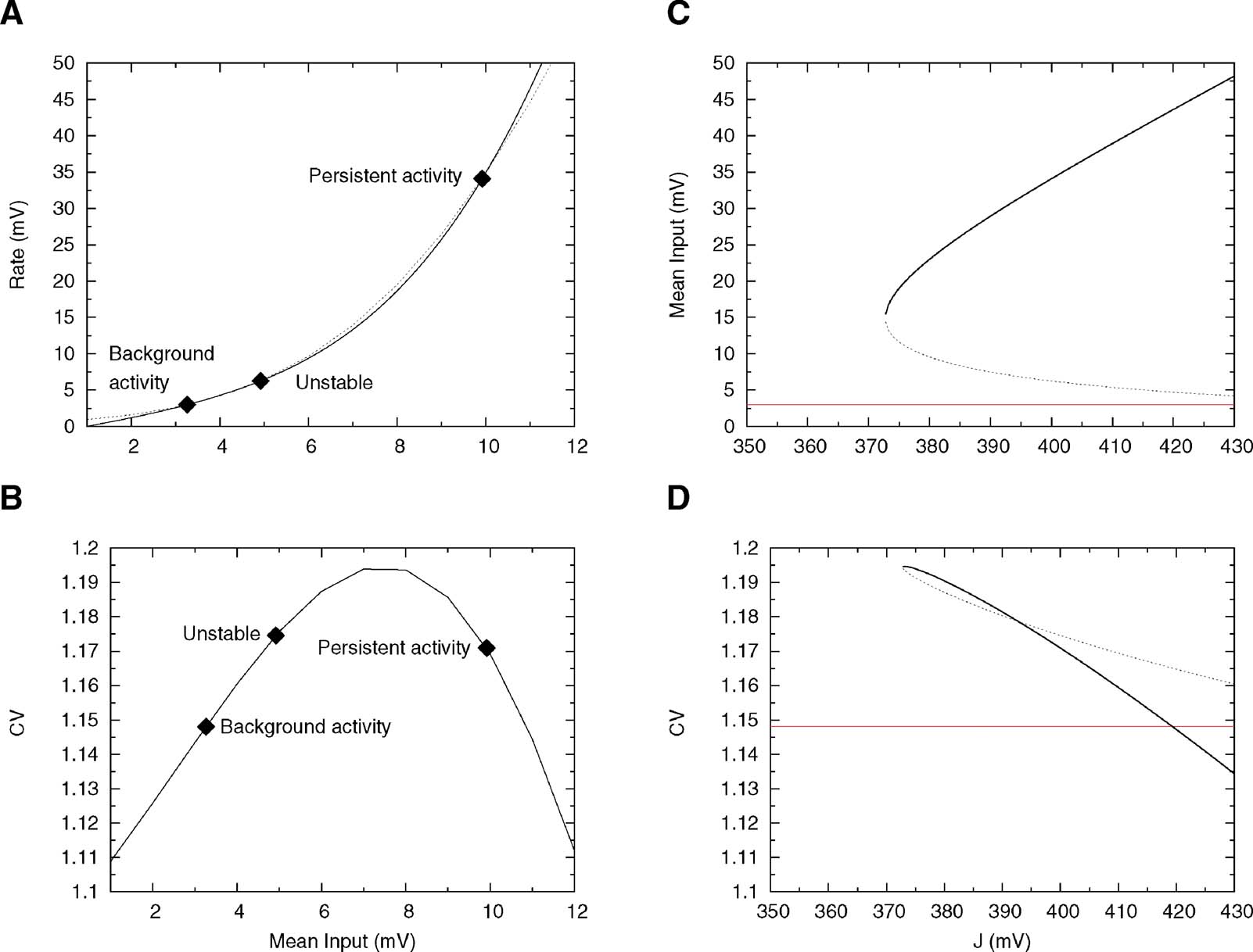
Figure 6. Single cell and network properties when neurons have high reset (V_r =  15 mV) and synapses have short-term depression. (A) f—I curve (solid line) plotted together with the current—rate relationship for synapses with short-term depression, Equation (33) (dotted curve). Intersections between these two curves (diamonds) yield the solutions of Equation (21). They correspond to background, unstable and persistent fixed points, respectively. (B) CV—I curve. Diamonds: Values of the CV for the three intersection points shown in A. (C) Bifurcation diagram showing firing rate versus J. The black curve correspond to the persistent state (stable), the dotted one to the boundary of the basin of attraction (unstable) and the red one to the background state (stable). ( D) CV versus J bifurcation diagram. There exists a finite range of values of the synaptic efficacy for which the CV in the persistent state is larger than in the background one (370 mV < J < 420 mV in the figure).

We tested the mean-field prediction using simulations of a network of 800 excitatory cells connected by synapses with STD. These simulations that the persistent state is stable only if the fraction of NMDA currents, γis high enough. If γ ≥ 0.8, the persistent activity is asynchronous and stable up to a value of J near the bifurcation point. On the other hand, if γ ≤ 0.7, for some value of J near the bifurcation point the asynchronous state destabilizes and network oscillations appear, with an amplitude that grows as γ decreases. When the amplitude of the resulting oscillation is large enough, persistent activity is destabilized. The value of the synaptic efficacy J at which the activity falls in the background state increases when γ decreases. These oscillations disappear for large values of J for everyγ. These oscillations are due to STD and have been observed previously in recurrent networks with frequency-dependent synapses (Tsodyks et al., 1998 ). Here, we used γ  =  0.9 for which the persistent activity is asynchronous and stable in a wide range of values of J. In Figure 7 B, we show the temporal evolution of the mean activity: in the pre-stimulus interval the network is in its background activity state and the CV is slightly larger than 1 (CV =  1.06); during the stimulus, short-term depression leads to a pronounced decrease in the activity (Chance et al., 1998 ; Mongillo et al., 2005 ), and during delay period the CV of the persistent activity reaches CV =  1.17, as predicted by the mean-field analysis. Figures 7 C and 7 D compare bifurcation diagrams for firing rates and CVs predicted by mean-field calculations with values obtained with simulations. Note the good agreement between the two; however, to reach such a good agreement, one needs to choose a very small value of the time step (dt =  1 μ s).

FIGURE 7

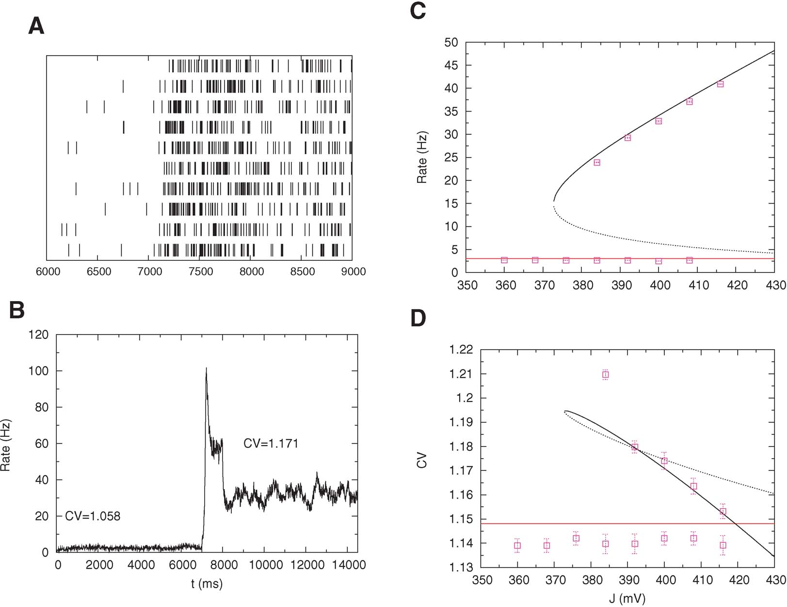
Figure 7. High CV in persistent activity: simulations versus mean-field. Pre-stimulus (0–7 second), stimulus (7–8 second) and post-stimulus (8–15 second) activity of a network of 800 excitatory cells with nonlinear synapses. (A) Spike trains of 10 neurons in the interval 6–9 second. (B) Mean network activity as a function of time (bins of 1 ms). The mean value of the CV in the persistent state is larger than in the pre-stimulus interval as predicted my mean-field. The transient decrease of the rate during the stimulus interval is due to short-term depression. (C) Bifurcation diagram showing firing rate versus excitatory coupling strength (mean-field: lines; simulations: symbols). (D) Bifurcation diagram showing CV versus excitatory coupling strength (mean-field: lines; simulations: symbols).

Effect of heterogeneity in reset potentials

Compte et al. (2003) classified PFC cells in three types of discharge patterns, ‘refractory’, ‘Poissonian’ and ‘bursty’ as assessed by their autocorrelograms and power spectra. They also found that the coefficients of variation of the spike trains of the three classes are such that the ‘refractory’ cells have the lowest CV, the ‘bursty’ ones have the highest CV, while the ‘Poissonian’ cells have a CV which is an intermediate between refractory and Poissonian.

To investigate whether heterogeneity can be responsible for this diversity of behaviours, we introduced in the model a variability in the reset potential from neuron to neuron. For each neuron, we draw randomly the reset potential using a uniform distribution between a minimum and a maximum value (we take mV and mV). We divided the whole population of neurons in three classes, according to the value of their reset potential (first class: V_r ∈ [10 mV, 13 mV); second class: V_r ∈ [13 mV, 16 mV), third class: V_r ∈ [16 mV, 19 mV)).

This heterogeneity leads to a large diversity in ISI histograms that reproduces qualitatively the diversity of ISI histograms found in Compte et al. (2003) , as shown in Figure 9 . The ISI histograms in the delay period are plotted for these three classes of neurons in Figure 9 . Neurons with high reset have a large peak close to the minimal ISI imposed by the refractory period (2 ms). This peak is much larger than a Poisson process with equivalent rate, indicating a tendency to fire in bursts, similar to the ‘bursty’ neurons found in PFC. On the other hand, neurons with low reset have a larger effective refractory period, as shown by the peak at larger ISIs (∼5 ms), similar to the ‘refractory’ neurons found in PFC. All these neurons have exponential tails of the ISI distribution, as shown in Figure 9 (note the logarithmic y scale in the graph). The CV distributions of these three classes of neurons are shown in Figure 8 , in both ‘fixation’ and ‘delay period’. It shows, as expected, that CV increases with reset potential.

FIGURE 8

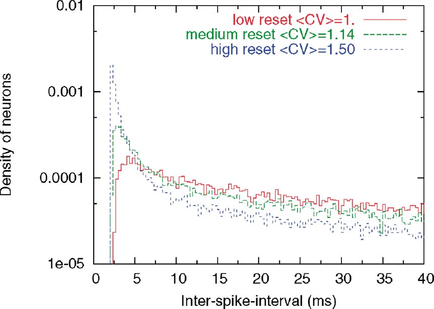
Figure 8. Hetereogenity of ISI distributions due to variability in the reset potentia. (A) Pre-stimulus interval (network in background state). Neurons with low reset (red curve) have a CV distribution centered below 1, due to the effective refractory period induced by the low reset. Neurons with large reset potential (blue curve) have high values of the CV. (B) Delay period (network in persistent state). There is an increase in the variability of the firing in all neuronal classes.

FIGURE 9

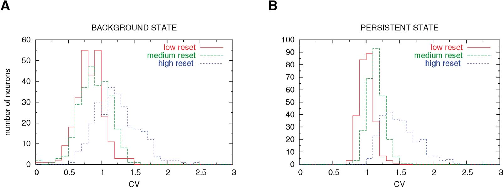
Figure 9. Distribution of CVs in the three classes of neuron. ISI histograms for three classes of neurons (low, intermediate and high V_r) during delay period. The y-axis is displayed in logarithmic scale. Note that the higher the reset, the larger the tendency to fire in bursts, leading to the pronounced peak close to the minimal ISI imposed by the refractory period (2 ms). On the other hand, neurons with lower resets have a longer effective refractory period, with a peak of the ISI distribution at ∼5 ms. These behaviours of the ISI histograms match qualitatively the three types of behaviours seen in Compte et al. (2003).

Spatial working memory model

So far we found that a network of excitatory neurons connected by synapses with STD is able to reproduce the irregularity of the persistent activity found in PFC. In this experiment, the authors recorded prefrontal neurons during an oculomotor delayed response (ODR) task in which neurons are spatially selective. Hence, in this section, we investigate whether these results still hold using a model with a spatial structure (Camperi and Wang, 1998 ; Compte et al., 2000 ; Renart et al., 2003 ) as described in ‘Materials and Methods’. The network we simulate is homogeneous (all neurons have the same reset).

The network activity is monitored by plotting its spatiotemporal firing pattern. Figure 10 A shows the rastergram of excitatory neurons labelled by the location of their preferred cues; during the ‘fixation’ period (0–2000 ms) the network is in the background state. After the cue presentation (2000–2500 ms), elevated persistent activity remains restricted to the group of neurons that received an increase in synaptic inputs during cue presentation throughout the delay period (2500–5500 ms). Figure 10 B shows the population firing profile, averaged over the delay period. Figure 10 C shows the CV profile, averaged over the delay period: the mean CV of neurons belonging to the subpopulation selective to the stimulus is 1.25.

FIGURE 10

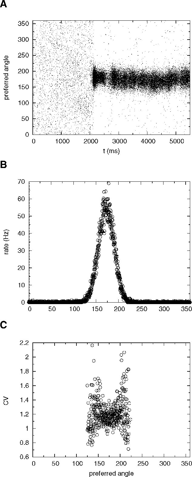
Figure 10. Spatial working memory network with J⁺ =  3.4. (A) Spike times of excitatory neurons, labelled by the location of their preferred cues. Fixation epoch (0–2000 ms): the entire excitatory population is in the background state. Stimulus presentation consists in enhancing the external input to neurons with preferred cues between [162, 198 degrees] during a period of 500 ms. This stimulus triggers a localized neural activity which persists during the delay period (2500–5500 ms). (B) Firing rate of single excitatory neurons in the delay period, as a function of preferred angle. (C) CV of single excitatory neurons in the delay period as a function of preferred angle. Only cells firing at more than 3 Hz are shown. Note the high irregularity of selective neurons in the delay period (mean CV is equal to 1.25).

Note that in this simulation we kept very low values of the background activity (ν _E =  0.75 Hz and ν_I =  2.5 Hz) in order to obtain a robust bistability. Using these values of ν_E and ν_I, we found selective persistent activity in the range J⁺ =  3.1−3.4 mV.

Figure 10 A also shows that the location of the bump exhibits small drifts around the location of the cue. This random drift is common to models with this type of architecture (see e.g. Compte et al., 2000 ; Renart et al., 2003 ). In fact, the order of magnitude of the displacement of the bump after 3 seconds is a few degrees, roughly of the same order of magnitude as reported in previous studies for a network of this size (Compte et al., 2000 ). Hence, the presence of short-term depression and strong irregularity of firing of cells participating in the bump does not affect adversely the stability of the bump.

Discussion

We have shown here that a purely excitatory network of spiking neurons can account for the high irregularity shown by PFC neurons in the delay period (Compte et al., 2003 ). In fact, in our model, persistent activity is even more irregular than background activity. Two conditions are necessary in our model to obtain this behaviour: (i) high post-spike reset, to obtain a non-monotonic CV—I curve; and (ii) saturation of average post-synaptic currents at high pre-synaptic firing rate, to allow persistent activity to occur in the high CV region. We now examine the evidence for these conditions to occur in PFC in vivo.

The first requirement is that the membrane potential should be reset after a spike above the mean membrane potential induced by fluctuating synaptic inputs. In particular, one should not see a pronounced hyperpolarization below that average membrane potential. This is a prediction of the model, that could be checked by intracellular recordings in PFC in vivo, which to our knowledge have never been performed. However, it is instructive to consider intracellular recordings in vivo in other cortical structures. Intracellular recordings in visual cortex of the cat have been performed by several groups in recent years. Visual inspection of the membrane potential traces shown e.g. by Anderson et al. (2000) and Monier et al. (2003) , for instance, seem to indicate no pronounced afterhyperpolarization, consistent with our prediction. Furthermore, one should expect that in a regime in which a neuron receives a large barrage of excitatory and inhibitory inputs, which has been hypothesized to be the situation in cortex, such inputs should decrease the effectiveness of potassium currents responsible for post-spike repolarization.

The second requirement is a saturation of the average post-synaptic currents at high pre-synaptic firing rate. Short-term depression leads to such a saturation (Tsodyks and Markram, 1997 ) and it is known to be present in excitatory-to-excitatory synapses in at least a subset of PFC neurons (Wang et al., 2006 ). Saturation at high presynaptic firing rates is in fact a general property of chemical synaptic transmission and is expected to occur regardless of the details of short-term dynamics.

Other studies (Sakai et al., 1999 ; Shinomoto et al., 1999 ) recently addressed the question of whether spike trains recorded in PFC during the delay period of a short-term memory task are well described by a LIF model with stochastic inputs. They show that the statistics of ISI can be reproduced by such a model, only if inputs are temporally correlated, with a correlation time constant of order 100 ms. In our model, stochastic external inputs were taken to be white noise for the sake of simplicity, but all our results should also hold with temporally correlated external inputs. In fact, the finite size of the network in our simulations leads to fluctuations of the recurrent inputs that have long correlation time constants, due to both the long NMDA decay, and to short-term depression time constants.

Electrophysiological recordings from PFC shows that cells in the delay period have often strongly non-stationary firing rates, which are not present in our model. This non-stationarity might in principle be another factor contributing to high CVs. To disambiguate between intrinsic variability of firing and variability due to temporal variations in firing rate, Compte et al. (2003) computed a ‘local’ measure of irregularity, the CV2, that measures irregularity from adjacent ISIs. Measured CV2s in PFC are also high (typically of order 1), showing that the observed irregularity is not due to non-stationarity of the firing rate.

In this paper, we have treated the standard deviation of the fluctuations in synaptic currents as a fixed parameter σ. The values of this parameter were chosen to be in the range of experimentally observed values in in vivo. The standard deviation of the distribution of membrane potentials in vivo has been reported to be approximately 5 mV (Anderson et al., 2000 ). This is roughly consistent with σ_ext =  8 mV, since at low firing rates, the standard deviation of the distribution of membrane potentials is approximately . Such a large variance is often thought to emerge due to strong excitation and inhibition that balance each other (Amit and Brunel, 1997 ; Tsodyks and Sejnowski, 1995 ; van Vreeswijk and Sompolinsky, 1996 , 1998 ).

Other investigators have proposed recently models with irregular persistent activity. These models rely on strong inhibition for such irregularity to emerge. Renart et al. (2007) showed strong irregularity of persistent activity when there is a balanced increase in both excitation and inhibition in the persistent state compared to the background state. In this scenario, the variance of synaptic inputs in the persistent state is significantly larger than the variance in the background state, explaining the high CV in the persistent state. However, the bistability range is small in this scenario, and it in fact vanishes in the limit of large number of connections per neurons (Renart et al., 2007 ). Another scenario involves a Hopfield-type memory structure on top of unstructured random excitatory connections (Roudi and Latham, 2007 ), together with inhibitory neurons maintaining a balance with excitation in both background and persistent states. The values of the CV obtained in that model are not very large—of the order of 0.8. However, it is important to note that the model they used, a quadratic integrate and fire neuron, is likely to behave as the LIF neuron if the reset potential is chosen to be close to threshold. We therefore believe that a high reset potential in the Roudi and Latham model, would lead to high CV (> 1) values in the persistent state, as found in our model.

We have demonstrated that high CVs occur robustly in an unstructured network. We have also performed preliminary simulations of a spatial working memory network, that also shows strong irregularity in persistent activity. A more detailed investigation of this model, as well as models storing an extensive number of discrete attractors, will be the subject of future work.

Acknowledgements

We are indebted to Daniel Amit, David Hansel and Gianluigi Mongillo for their insightful comments on a previous version of the manuscript.

References

Alili, L., Patie, P., and Pedersen, J. (2005). Representations of the first hitting time density of an Ornstein-Uhlenbeck process. Stoch. Models 21, 967–980.

Amit, D. J., and Brunel, N. (1997). Model of global spontaneous activity and local structured activity during delay periods in the cerebral cortex. Cereb. Cortex 7, 237–252.

Pubmed Abstract | Pubmed Full Text

Amit, D. J., and Tsodyks, M. V. (1991). Quantitative study of attractor neural network retrieving at low spike rates I: Substrate—spikes, rates and neuronal gain. Network 2, 259–274.

Anderson, J. S., Lampl, I., Gillespie, D. C., and Ferster, D. (2000). The contribution of noise to contrast invariance of orientation tuning in cat visual cortex. Science 290, 1968–1972.

Pubmed Abstract | Pubmed Full Text

Brunel, N. (2000). Persistent activity and the single cell f-I curve in a cortical network model. Network 11, 261–280.

Pubmed Abstract | Pubmed Full Text

Brunel, N. (2004). Network models of memory. In Methods and Models in Neurophysics, Les Houches 2003, C. Chow, B. Gutkin, D. Hansel, C. Meunier, J. Dalibard, eds. (Elsevier, London).

Brunel, N., and Wang, X. J. (2001). Effects of neuromodulation in a cortical network model of object working memory dominated by recurrent inhibition. J. Comput. Neurosci. 11, 63–85.

Pubmed Abstract | Pubmed Full Text

Camperi, M., and Wang, X.-J. (1998). A model of visuospatial short-term memory in prefrontal cortex: recurrent network and cellular bistability. J. Comput. Neurosci. 5, 383–405.

Pubmed Abstract | Pubmed Full Text

Chance, F. S., Nelson, S. B., and Abbott, L. F. (1998). Synaptic depression and the temporal response characteristics of V1 cells. J. Neurosci. 18, 4785–4799.

Pubmed Abstract | Pubmed Full Text

Compte, A., Brunel, N., Goldman-Rakic, P. S., and Wang, X.-J. (2000). Synaptic mechanisms and network dynamics underlying spatial working memory in a cortical network model. Cere. Cortex 10, 910–923.

Pubmed Abstract | Pubmed Full Text

Compte, A., Constantinidis, C., Tegnér, J., Raghavachari, S., Chafee, M., Goldman-Rakic, P. S., and Wang, X.-J. (2003). Temporally irregular mnemonic persistent activity in prefrontal neurons of monkeys during a delayed response task. J. Neurophysiol. 90, 3441–3454.

Pubmed Abstract | Pubmed Full Text

Funahashi, S., Bruce, C. J., and Goldman-Rakic, P. S. (1989). Mnemonic coding of visual space in the monkey's dorsolateral prefrontal cortex. J. Neurophysiol. 61, 331–349.

Pubmed Abstract | Pubmed Full Text

Fuster, J. M., and Alexander, G. (1971). Neuron activity related to short-term memory. Science 173, 652–654.

Pubmed Abstract | Pubmed Full Text

Fuster, J. M., and Jervey, J. P. (1981). Inferotemporal neurons distinguish and retain behaviourally relevant features of visual stimuli. Science 212, 952–955.

Pubmed Abstract | Pubmed Full Text

Goldman-Rakic, P. S. (1995). Cellular basis of working memory. Neuron 14, 477–485.

Pubmed Abstract | Pubmed Full Text

Honeycutt, R. L. (1992). Stochastic Runge-Kutta algorithms. I. White noise. Phys. Rev. A 45, 600–603.

Pubmed Abstract | Pubmed Full Text

Miyashita, Y. (1988). Neuronal correlate of visual associative long-term memory in the primate temporal cortex. Nature 335, 817–820.

Pubmed Abstract | Pubmed Full Text

Mongillo, G., Curti, E., Romani, S., and Amit, D. J. (2005).Learning in realistic networks of spiking neurons and spike-driven plastic synapses. Eur. J. Neurosci. 21, 3143–3160.

Pubmed Abstract | Pubmed Full Text

Monier, C., Chavane, F., Baudot, P., Graham, L. J., and Fregnac, Y. (2003). Orientation and direction selectivity of synaptic inputs in visual cortical neurons: a diversity of combinations produces spike tuning. Neuron 37, 663–680.

Pubmed Abstract | Pubmed Full Text

Nakamura, K., and Kubota, K. (1995). Mnemonic firing of neurons in the monkey temporal pole during a visual recognition memory task. J. Neurophysiol. 74, 162–178.

Pubmed Abstract | Pubmed Full Text

Renart, A. Multi-modular memory systems. (2000). Ph.D. Thesis, Universidad AutÓnoma de Madrid.

Renart, A., Moreno, R., and Wang, X. J. (2003). Robust spatial working memory through homeostatic synaptic scaling in heterogenous cortical networks. Neuron 38, 473–485.

Pubmed Abstract | Pubmed Full Text

Renart, A., Moreno-Bote, R., Wang, X.-J., and Parga, N. (2007). Mean-driven and fluctuation-driven persistent activity in recurrent networks. Neural Comput. 19, 1–46.

Pubmed Abstract | Pubmed Full Text

Ricciardi, L. M. (1977). Diffusion processes and related topics on biology (Berlin, Springer-Verlag).

Romani, S., Amit, D. J., and Mongillo, G. (2006). Mean-field analysis of selective persistent activity in presence of short-term synaptic depression. J. Comput. Neurosci. 20, 201–217.

Pubmed Abstract | Pubmed Full Text

Roudi, Y., and Latham, P. E. A balanced memory network. (2007). early online release.

Pubmed Abstract | Pubmed Full Text

Sakai, Y., Funahashi, S., and Shinomoto, S. (1999). Temporally correlated inputs to leaky integrate-and-fire models can reproduce spiking statistics of cortical neurons. Neural Netw. 12, 1181–1190.

Pubmed Abstract | Pubmed Full Text

Shinomoto, S., Sakai, Y., and Funahashi, S. (1999). The Ornstein-Uhlenbeck process does not reproduce spiking statistics of neurons in prefrontal cortex. Neural Comput. 11, 935–951.

Pubmed Abstract | Pubmed Full Text

Troyer, T. W., and Miller, K. D. (1997). Physiological gain leads to high ISI variability in a simple model of a cortical regular spiking cell. Neural Comput. 9, 971–983.

Pubmed Abstract | Pubmed Full Text

Tsodyks, M. V., and Markram, H. (1997). The neural code between neocortical pyramidal neurons depends on neurotransmitter release probability. Proc. Natl. Acad. Sci. USA 94, 719–723.

Pubmed Abstract | Pubmed Full Text

Tsodyks, M. V., Pawelzik, K., and Markram, H. (1998). Neural networks with dynamic synapses. Neural Comput. 10, 821–835.

Pubmed Abstract | Pubmed Full Text

Tsodyks, M. V., and Sejnowski, T. (1995). Rapid state switching in balanced cortical network models. Network 6, 111–124.

van Vreeswijk, C., and Sompolinsky, H. (1996). Chaos in neuronal networks with balanced excitatory and inhibitory activity. Science 274, 1724–1726.

Pubmed Abstract | Pubmed Full Text

van Vreeswijk, C., and Sompolinsky, H. (1998). Chaotic balanced state in a model of cortical circuits. Neural Comput. 10, 1321–1371.

Pubmed Abstract | Pubmed Full Text

Wang, Y., Markram, H., Goodman, P. H., Berger, T. K., Ma, J., and Goldman-Rakic, P. S. (2006). Heterogeneity in the pyramidal network of the medial prefrontal cortex. Nat. Neurosci. 9, 534–542.

Pubmed Abstract | Pubmed Full Text