 Takeshi Okuzono
 Takumi Yoshida
- 1Environmental Acoustic Laboratory, Department of Architecture, Graduate School of Engineering, Kobe University, Kobe, Japan
- 2Technical Research Institute, Hazama Ando Corporation, Tsukuba, Japan
Applicability of wave-based acoustics simulation methods in the time domain has increased markedly for performing room-acoustics simulation. They can incorporate sound absorber effects appropriately with a local-reaction frequency-dependent impedance boundary condition and an extended-reaction model. However, their accuracy, efficiency and practicality against a standard frequency-domain solver in 3D room acoustics simulation are still not known well. This paper describes a performance examination of a recently developed time-domain FEM (TD-FEM) for small-room acoustics simulation. This report first describes the significantly higher efficiency of TD-FEM against a frequency-domain FEM (FD-FEM) via acoustics simulation in a small cubic room and a small meeting room, including two porous-type sound absorbers and a resonant-type sound absorber. Those sound absorbers are modeled with local-reaction frequency-dependent impedance boundary conditions and an extended-reaction model. Then, the practicality of time-domain FEM is demonstrated further by simulating the room impulse response of the meeting room under various sound absorber configurations, including the frequency component up to 6 kHz. Results demonstrated the high potential and computational benefit of time-domain FEM as a 3D small room acoustics prediction tool.
1 Introduction
Computational room-acoustics simulation methods (Vorländer, 2013; Sakuma et al., 2014) are crucially important technologies for designing comfortable indoor sound environments in architectural spaces such as concert halls and classrooms. Two acoustic simulation methods are available to compute room-impulse responses (RIR): wave-acoustics and geometrical-acoustics methods. The RIRs are essential quantities for room-acoustics evaluation and room-acoustics auralization, but the two simulation methods have their respective and opposite strengths and weaknesses. Wave-acoustics methods are a rigorous simulation technology offering higher reliability for prediction accuracy because they solve wave equations or Helmholtz equations using numerical methods such as finite element method (FEM) and boundary element method (BEM). Wave-acoustics methods are adversely affected by their high computational loads for practical applications, but their applicable scale of space and frequency range is expanding dramatically with advances in computational technology. Conversely, geometrical-acoustics methods (Savioja and Svensson, 2015) such as ray tracing methods have high capability for practical room-acoustics design with low computational loads because they deal with sound wave propagation as ray propagation where wave effects such as diffraction are neglected. This simplification naturally reduces the prediction accuracy, but a continuous effort has been undertaken to increase their accuracy. This report presents a discussion of the applicability of a recently developed wave-acoustics method in time-domain to 3D room-acoustics simulation.
Room acoustics simulation using wave-acoustics methods has been performed respectively in both the frequency-domain and time-domain, solving the Helmholtz and wave equations. Both methods in a different domain also have unique strengths and weaknesses. FEM (Otsuru et al., 2000; Otsuru et al., 2001; Okamoto et al., 2007; Aretz and Vorländer, 2014; Okuzono and Sakagami, 2018; Murillo et al., 2019; Hoshi et al., 2020; Yatabe and Sugahara, 2022) and BEM (Yasuda et al., 2016; Yasuda et al., 2020; Gumerov and Duraiswami, 2021; Cardoso Soares et al., 2022) are standard selection as a numerical method in the former frequency-domain simulations. Frequency-domain (FD) methods have an inherent benefit for use in modeling sound absorbers (Cox and Peter, 2017) such as porous-type and resonant-type materials accurately: they can deal naturally with complex-valued frequency-dependent quantities such as specific acoustic admittance. This capability is an important advantage in computing accurate RIR, including sound absorber effects. However, FD methods need multi-frequency analyses that solve linear system equations at each pure tone analysis for RIR calculations. The solution is still quite time-consuming for large-scale room-acoustic problems at higher frequencies.
A wide variety of numerical methods are available for time-domain simulations: finite-difference time-domain (FDTD) (Sakamoto, 2007; Kowalczyk and van Walstijn, 2008; Sakamoto et al., 2008; Kowalczyk and van Walstijn, 2011; Hamilton and Bilbao, 2017; Toyoda and Eto, 2019; Cingolani et al., 2021; Toyoda and Sakayoshi, 2021) or finite-volume time-domain (FVTD) methods (Bilbao, 2013; Bilbao et al., 2016), time-domain BEM (TD-BEM) (Hargreaves and Cox, 2008), time-domain FEM (TD-FEM) (Okuzono et al., 2019; Yoshida et al., 2022), time-domain discontinuous Galerkin FEM (DG-FEM) (Simonaho et al., 2012; Wang et al., 2019; Wang and Hornikx, 2020; Pind et al., 2021), time-domain spectral element method (TD-SEM) (Pind et al., 2019), pseudospectral time-domain (PSTD) method (Hornikx et al., 2015; Hornikx et al., 2016), and adaptive rectangular decomposition (ARD) method (Mehra et al., 2012; Morales et al., 2015; Rabisse et al., 2019). They respectively offer several benefits in terms of ease of coding and applicability of complex geometries and so on according to fundamental algorithms of numerical methods. Time-domain (TD) methods are particularly useful for computing RIR because they can obtain time responses that include a broad frequency range with a single computational run. Moreover, they can be designed as a faster explicit solver, although more stable and accurate implicit methods are available. An inherent shortcoming of TD methods is their difficulty in addressing frequency-dependent quantities. To address this inefficiency, accurate sound absorber modeling in the time domain is an active research topic which, if resolved, can increase the methods’ applicability to room-acoustics simulation. Consequently, some TD methods which can deal accurately with effects of sound absorbers have been developed by incorporating local-reaction frequency-dependent impedance boundary conditions (Sakamoto et al., 2008; Bilbao, 2013; Pind et al., 2019; Rabisse et al., 2019; Wang and Hornikx, 2020; Okuzono et al., 2021). Extended-reaction models, which are naturally available in FD methods, have also been presented to deal further with the sound incidence-angle dependence effect for some porous sound materials (Okuzono et al., 2019; Zhao et al., 2019; Pind et al., 2020; Yoshida et al., 2020). Therefore, current TD methods are becoming attractive simulation technologies for room acoustics simulation.
Nevertheless, the applicability of current TD methods to 3D room-acoustics simulation considering realistic sound absorbers configurations has not been discussed well. More specifically, the accuracy, efficiency, and utility of recent TD methods against FD methods remain unclear. To elucidate several aspects of these methods, this study specifically examines a recently developed TD-FEM (Okuzono et al., 2019; Okuzono et al., 2021) for 3D room-acoustics simulation among earlier described TD methods and discusses the question with some case studies of small room-acoustics scenarios. Because TD-FEM is generally regarded as computationally expensive compared to the most used FDTD method, a case study will demonstrate a practical room acoustic simulation scenario with various sound absorber configurations at a broad frequency range beyond 4 kHz, where human auditory sensitivity has its peak.
The purpose of this study is to discuss the potential of the recently-developed TD-FEM on 3D room-acoustics simulation. To this end, this paper examines the efficiency and accuracy of TD-FEM by the performance comparison with a 3D frequency-domain FEM(FD-FEM) that uses the same finite elements for spatial discretization. The examination is performed via room acoustic simulations in a small cubic room and a small meeting room. The practicality of TD-FEM is evaluated through a case study of room acoustics simulation in a small meeting room up to 6 kHz under realistic sound absorber configurations. The present paper deals with three sound absorbers: a local-reaction glass wool (GW) and extended-reaction acoustic fabric curtains (AF) as porous sound absorbers and a local-reaction microperforated panel (MPP) absorber as resonant-type sound absorbers. This study is an extension of our earlier work (Okuzono et al., 2021) on 2D room-acoustics simulation. In the previous study, we examined the performance of TD-FEM against FD-FEM via acoustics simulations of a 2D office and a concert hall with GW absorbers modeled by the frequency-dependent impedance boundary conditions. The result revealed that TD-FEM has higher efficiency with about 18 times faster computational speed than FD-FEM on 2D room-acoustics simulation. However, whether or not 2D simulation results hold to 3D simulations is unclear. Therefore, it is extremely important to show evidence of the higher efficiency of TD-FEM on 3D room-acoustics simulation. The present study also includes an accuracy examination of room-acoustic parameters from a practical aspect, which are not tested in the previous study. As the salient point of novelty of the present work, we reveal that 3D TD-FEM engenders a substantial performance gain on room-acoustics simulation compared to 3D FD-FEM-based prediction and its practicality as a prediction tool for designing the acoustics of small rooms. Notably, the performance gain is one magnitude greater than that in 2D simulations. To the best of the authors’ knowledge, the present paper is the first to reveal the high potential of TD-FEM against FD-FEM in 3D room-acoustics simulations with realistic sound absorber modeling that uses a complex-valued specific acoustic admittance and an extended-reaction model. Since TD-FEM can be extended from a standard FD-FEM code, the presented results give FD-FEM users an alternative way to perform room-acoustics simulation more efficiently.
2 Room acoustic simulation using FEM
This report presents a dispersion-reduced TD-FEM and FD-FEM with a frequency-dependent local-reaction boundary condition and an extended-reaction model for permeable membrane absorbers such as AF (Okuzono and Sakagami, 2015; Okuzono and Sakagami, 2018; Okuzono et al., 2019; Okuzono et al., 2021). The spatial domain is discretized with dispersion-reduced eight-node hexahedral finite elements (Hex8), which uses Gauss–Legendre rules with modified integration points (Guddati and Yue, 2004; Yue and Guddati, 2005) to reduce spatial discretization error. As a notable feature, the dispersion-reduced FEMs can provide a more accurate solution than FEMs using conventional Hex8 for a coarser mesh (Okuzono and Sakagami, 2018; Okuzono et al., 2019). Supplementary Section S1 explains this aspect from theoretical discretization error evaluation as a fundamental. For the convenience of the reader, we briefly describe the basic equations of TD-FEM and FD-FEM used here. The sound absorber model used for the frequency-dependent local-reaction boundary condition is also given. Detailed formulations of the dispersion-reduced TD-FEM and FD-FEM are available in the literature (Okuzono and Sakagami, 2015; Okuzono and Sakagami, 2018; Okuzono et al., 2019; Okuzono et al., 2021).
2.1 Time-domain FEM
Time-domain room acoustics simulation solves the following inhomogeneous acoustic wave equation to simulate sound propagation in a 3D enclosed space Ω as
where p stands for the sound pressure at the position vector r = (x, y, z) in Cartesian coordinate system at time t, c denotes the speed of sound in air, ρ expresses the air density. The symbol ∇2 is the Laplacian;
As described earlier, the present paper presents consideration of three sound absorbers. The GW and MPP absorbers are modeled by the local-reaction (LR) frequency-dependent absorbing boundary condition (BC), which is defined on the sound absorbing surface Γa as
where
where ΓAF,1 and ΓAF,2 respectively represent boundaries in both sides of curtain, and where vf represents the particle velocity on and inside the AF, which is defined as
where σ, tAF, and MAF respectively represent the flow resistivity, and the thickness and the surface density of AF, and Δp is the sound pressure difference between both sides of AF.
By applying finite element discretization to the weak form of Eq. 1 with those 2 BCs, we obtain the following semi-discretized matrix equation as
where three matrices M, K, and C′ respectively stand for the global mass matrix, the global stiffness matrix, and the global dissipation matrix without the admittance term. A matrix S denotes the global matrix related to AF. Two vectors p and f represent the sound pressure vector and the external force vector. Parameters y∞, Ai, Bi, and Ci are the real-valued coefficients for the following rational function approximation of
with Nrp real poles λi and Ncp complex conjugate poles αi ± jβi. The vectors ϕi,
We use Crank–Nicolson method with a high stability as the ODE solver. The sound pressure is computed by solving the second-order ODE of Eq. 5. We use the high-accuracy Fox–Goodwin method (Hughes, 2000) for the solution of Eq. 5. The present TD-FEM formulation has an implicit algorithm. Therefore, the linear system of equations at each time step is solved using a Krylov subspace iterative method called Conjugate Gradient (CG) method (Barrett et al., 1994) with diagonal scaling preconditioning. The convergence tolerance, which determines the resulting accuracy on solutions, is set as 10–4. The rational function models of GW and MPP absorbers are constructed using normal-incidence specific acoustic admittance ratio calculated using the transfer matrix method. As for numerical operations of TD-FEM, all computations are performed with real-valued operations, i.e., all matrices and vectors have real-valued components. An efficient sparse matrix storage format, namely the compressed row storage format, is used for storing matrices, which requires the largest memory consumption in FEM. The most time-consuming operation in TD-FEM is real-valued sparse matrix-vector products, which mainly appear in the linear system solution process by CG method at each time step. CG method has one sparse matrix-vector product per iteration. Therefore, the fast convergence of iterative solvers with small iteration numbers is an essential factor in achieving higher computational performance. Also, the iteration number required for convergence becomes a good quantity for the performance evaluation of the present TD-FEM.
2.2 Frequency-domain FEM
Frequency-domain room acoustics simulation solves the following inhomogeneous Helmholtz equation to simulate complex-valued sound pressure
where k represents the wavenumber in air and the symbol
In FD-FEM, we also use the normal-incidence specific acoustic admittance ratio calculated using the transfer matrix method to GW and MPP absorbers.
The following interior boundary condition is also used to model AF as
with the transfer admittance
Applying finite element discretization to the weak form of Eq. 10 produces the following linear system of equations as (Okuzono and Sakagami, 2015)
where
2.3 Sound absorber modeling with transfer matrix method
When using LR BCs, the complex-valued specific acoustic admittance ratio of the sound absorber must be known. Both theoretical and measurement-based approaches are available to obtain the specific acoustic admittance ratio of materials. Measurement-based approaches include an impedance tube measurement (ISO 10534-2, 1998) and in-situ measurements (Brandão et al., 2015; Sakamoto et al., 2018; Sugahara et al., 2019). The transfer matrix method is a general way to theoretically compute the sound absorption characteristics of materials, and well-developed models are available for GW and MPP absorbers. This report presents computation of the specific acoustic admittance ratio by the transfer matrix method (Allard and Atalla, 2009) to model GW and MPP absorbers as frequency-dependent LR BCs. Here, the MPP absorber is a single-leaf MPP backed by a GW. We designate this absorber as MPPGW. For plane wave incidence at the angle θ, the transfer matrix TP of the porous material is
with
However, the transfer matrix TM of MPP is represented by a lumped element as
where Zt is the transfer impedance of MPP. For a limp MPP, the transfer impedance is defined as (Sakagami et al., 2005)
where Zmpp denotes the specific acoustic impedance of rigid MPP and Mmpp represents the surface density of MPP. We use Maa’s impedance model (Maa, 1987) as Zmpp. The total transfer matrix T of MPPGW absorber is calculated as
Assuming rigid termination, the specific acoustic admittance ratio
Those
3 Accuracy and efficiency of TD-FEM against FD-FEM
This section presents a discussion of how accurate and efficient 3D TD-FEM is against 3D FD-FEM with two case studies. As notable results, we report the marked performance gain of the time-domain solver against the frequency-domain solver on room-acoustics simulation. The first case study, described in Section 3.1, performs the accuracy and efficiency examination via sound field analysis in a small cubic room of 1.01 m3 including three sound absorbers. Figure 1A depicts the small cubic room model. The accuracy examination is based on comparison of frequency responses computed using both methods under the same spatial resolution meshes. One can expect TD-FEM to have a similar level of accuracy as in FD-FEM when time-domain LR BCs model the frequency-dependence of sound absorbers successfully because both methods have almost identical discretization error characteristics to those shown in our earlier work (Okuzono et al., 2021) and Supplementary Section S1. The computational cost comparison evaluates their efficiency. Then, the second case study in Section 3.2 uses a more realistic meeting room model of 68 m3 as presented in Figure 1B. In the meeting room model study to show the practical accuracy of impulse responses computed by TD-FEM, we further compare four room-acoustic parameters computed by both methods: reverberation time (T20), early decay time (EDT), clarity of speech (C50), and sound strength (G). As described in the preceding section, we also compared the computational cost between PARDISO and CSQMOR methods. All computations were done using a computer (Mac Pro 2020; Apple Inc., Xeon CPU W 2.7 GHz, 24 cores; Intel Corp.) with a Fortran compiler (ver. 2020; Intel Corp.). The FEM programs used for this study were created by the authors using in-house code.
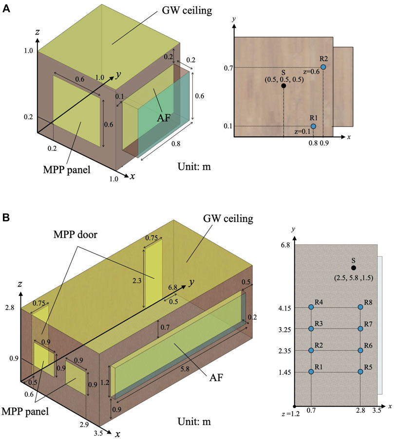
FIGURE 1. Room models: (A) Small room of 1.01 m3 with a source S and two receivers R1 and R2; and (B) Meeting room of 68 m3 with a source S and eight receivers R1–R8. Both rooms include GW absorber on ceiling, MPP absorber on walls, and AF absorber in front of a window. The Meeting room further includes MPP absorbers as doors.
3.1 Small cubic room model
3.1.1 Problem description and numerical setup
We computed the sound field generated by sound radiation from a monopole source in a small cubic room, as shown in Figure 1A at frequencies up to 3 kHz, with TD-FEM and FD-FEM. This room has three sound absorbers: a GW absorber on the ceiling, an AF in front of the window, and an MPPGW absorber on a wall. The GW absorber has flow resistivity R = 55,000 Pa s/m2 with 25 mm thickness. MPPGW absorber uses the same GW behind an MPP leaf with 1.13 kg/m3 surface density, 1 mm hole diameter, 1 mm panel thickness, and 9 mm plate pitch. The AF has surface density of 0.5 kg/m2 and flow resistance of 416 Pa s/m. Figures 2A–C show their random incidence sound absorption coefficient αr computed using the transfer matrix method. This figure includes both αr computed assuming LR and ER for GW and MPPGW absorbers to show how the LR assumption used for the numerical analysis fits the exact ER model. The other surfaces assigned the specific acoustic admittance ratio
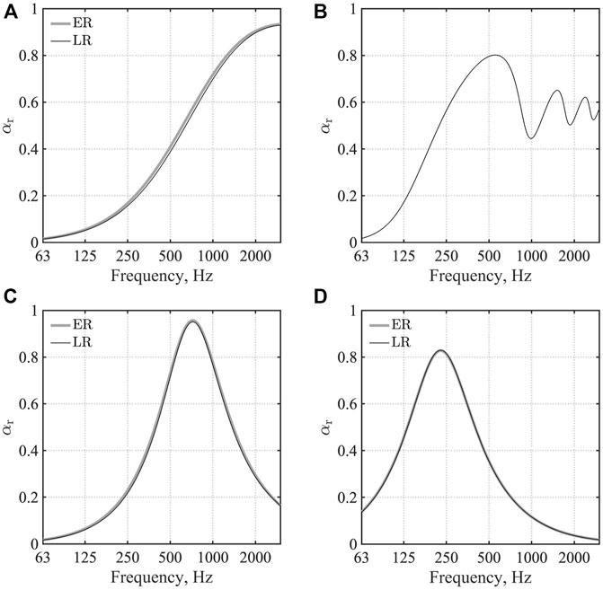
FIGURE 2. Random incidence sound absorption coefficient: (A) GW ceiling; (B) AF; (C) MPPGW panel; and (D) MPPGW door. ER and LR respectively denote extended reaction model and local reaction model.
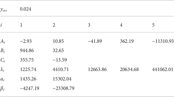
TABLE 1. Parameters y∞, Ai, Bi, Ci, λi, αi, and βi for MPPGW panel. The parameters were fitted at 10 Hz—10 kHz.
For spatial discretization, we used Hex8 with dispersion reduced TD-FEM and FD-FEM. The resulting FE mesh has 146,632 degrees of freedom (DOF), using cubic elements of 0.02 m edge length for the air domain and rectangular elements of 0.001 m × 0.02 m × 0.02 m for AF. The spatial resolution of FE mesh is 5.7 elements per wavelength at the upper-limit frequency of 3 kHz, where the spatial resolution is defined as the ratio between the wavelength and the maximum edge length. There exist a well-used rule of thumb, i.e., ten elements per wavelength, for the spatial discretization using linear elements. As described in Supplementary Section S1, compared to the standard FEMs using a mesh that follows the rule of thumb, the dispersion-reduced FEMs can provide a more accurate solution with a coarser mesh with about five elements per wavelength. According to the fact, the present paper created the FE mesh. A source S and two receivers R1 and R2 are placed respectively at positions (0.5, 0.5, 0.5), (0.8, 0.1, 0.1), and (0.9, 0.7, 0.6). For time-domain simulation, we used the impulse response of an optimized FIR filter based on the Parks–McClellan algorithm as a sound source signal
To compare the frequency responses SPL (r, ω) computed by both methods, for TD-FEM results, we compute its transfer function value using the following equation, removing the sound source characteristics
where
where LFD (fc, ri), and LTD (fc, ri) respectively represent the 1/3 octave band SPLs at center frequency fc at receiver’s position ri computed by FD-FEM and TD-FEM, and where nreceiver is the number of receivers.
3.1.2 Results
Figures 3A,B respectively present comparisons of frequency responses at R1 computed using TD-FEM and FD-FEM. For FD-FEM results, we designated the case using the sparse direct solver PARDISO as FD-FEM(Direct) and the case using the iterative solver CSQMOR as FD-FEM(Iterative). As a fundamental feature, we find that frequency responses become flattened at higher frequencies because of the higher sound absorption of porous type sound absorbers GW and AF. Two frequency responses by TD-FEM and FD-FEM show excellent agreement irrespective of the type of linear system solvers in FD-FEM. These results indicate that TD-FEM can accurately model the sound absorption characteristics of GW, MPPGW, and AF absorbers. The TD-FEM result fits better with the FD-FEM result obtained using the direct solver, which has better accuracy than those of iterative solvers. Some discrepancies can be found in SPL dips at frequencies below 700 Hz when using the iterative solver in FD-FEM. These discrepancies at dips were discussed in earlier reports of the literature (Okamoto et al., 2007) describing the performance of another iterative solver applied to high-order FD-FEM. We infer that FD-FEM using an iterative solver has difficulty computing a converged solution at dips in SPL, although this error property is unimportant from a practical perspective. It is particularly interesting that the TD-FEM result shows good agreement with FD-FEM(Direct), even when using an iterative solver. The discrepancy between TD-FEM and FD-FEM at a dip around 2,700 Hz is attributable to their slight differences in discretization error characteristics.
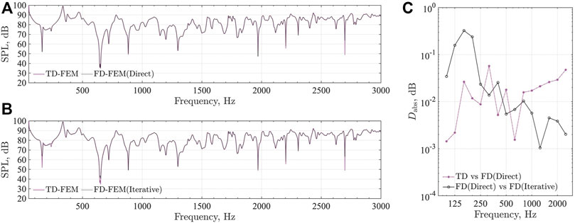
FIGURE 3. Comparison of frequency responses at R1 between TD-FEM and FD-FEM using sparse direct solver and iterative solver, and the absolute difference between them in
Figure 3C shows the absolute difference Dabs in 1/3 octave band SPL between TD-FEM and FD-FEM(Direct). This figure also includes Dabs between FD-FEM(Direct) and FD-FEM(Iterative) to emphasize the differences in accuracies of the different linear system solvers. Results revealed that the 1/3 octave band SPL between TD-FEM and FD-FEM(Direct) match well within the absolute difference of 0.06 dB, showing that the two methods have comparable accuracy. Regarding the two FD-FEM results obtained using different linear system solvers, 1/3 octave band SPL between FD-FEM(Direct) and FD-FEM(Iterative) also agree well below Dabs = 0.3 dB, which indicates that the iterative solver has sufficient accuracy from a practical perspective. Slightly larger absolute differences at 125 Hz–200 Hz are attributable to discrepancies at the dips.
Computational cost comparisons revealed TD-FEM as the fastest method for serial and parallel computations, with noteworthy performance. Actually, in terms of serial computation, TD-FEM is, respectively about 68 and 27 times faster than FD-FEM(Direct) and FD-FEM(Iterative). Results show that TD-FEM, FD-FEM(Direct) and FD-FEM(Iterative) took, respectively 1,067 s, 72,279 s, and 28,632 s to produce a solution. This marked performance benefit provided by TD-FEM derives from an iterative solver’s markedly better convergence property for a linear system solution. Actually, TD-FEM required only a mean iteration number of 5.6 per time step, whereas FD-FEM(Iterative) required 965.7 iterations per frequency. The TD-FEM only required the iteration of
3.2 Meeting room model
3.2.1 Problem description and numerical setup
We computed the sound field in a meeting room (Figure 1B) at frequencies up to 1.6 kHz. This room includes four sound absorbers: a GW ceiling absorber, an AF in front of the window, two MPPGW wall panels, and two MPPGW doors. It is noteworthy that MPPGW panels and MPPGW doors have different resonant frequencies. The GW, AF, and MPPGW panels have the same sound absorption characteristics used in earlier small room model studies. The MPPGW doors comprise a rigid MPP leaf with 1 mm hole diameter, 2 mm plate thickness, 15 mm pitch, and a backing 50-mm-thick GW absorber with the flow resistivity R = 55,000 Pa s/m2. Figure 2D shows the random incidence sound absorption coefficient αr computed using the transfer matrix method. Results show that the LR assumption is also valid for MPPGW door. Its rational function form for TD-FEM is shown in Table 2. Other surfaces were treated as reflective surfaces with
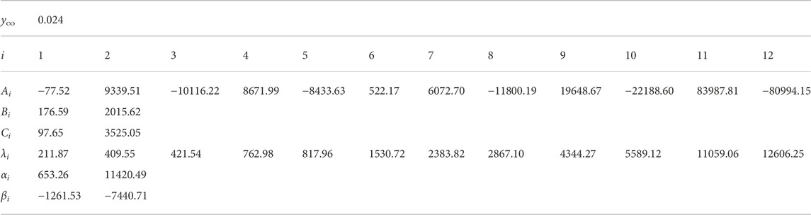
TABLE 2. Parameters y∞, Ai, Bi, Ci, λi, αi, and βi for MPPGW door. The parameters were fitted at 50 Hz—2 kHz.
Spatial discretization was performed with cubic Hex8 of 0.05 m edge length. The resulting FE mesh has 569,064 DOF, with spatial resolution of 4.9 elements per wavelength at 1.4 kHz. Sound source placement was at a point S (2.5, 5.8, 1.5). Also, eight receivers were placed at positions R1–R8, as shown in Figure 1B. TD-FEM uses an impulse response of optimized FIR filter based on the Parks–McClellan algorithm as the sound source signal
Four room-acoustic parameters were calculated from RIRs using TD-FEM and FD-FEM according to ISO 3382–1 (ISO 3382-1, 2009): T20, EDT, G, and C50. For FD-FEM, the RIR is computed using the inverse Fourier transform with the source spectrum
with the spatial averaged T20 (fc) computed using FD-FEM and TD-FEM at each octave band center frequency, respectively denoting
where EDTFD (fc, ri) and EDTTD (fc, ri) respectively denote EDT computed using FD-FEM and TD-FEM at receiver’s position ri. For G and C50, we defined the absolute difference as
where GFD (fc, ri), and GTD (fc, ri) represents G values computed by FD-FEM and TD-FEM, and
3.2.2 Results
Figure 4 presents a comparison of frequency responses at R1, as computed by TD-FEM and FD-FEM using PARDISO. The two frequency responses mutually match well at all frequency ranges. Regarding the reference, Figure 5 depicts 1 octave band SPL distributions at 500 Hz and 1 kHz in the meeting room. At the room’s boundaries, SPL is lower on surfaces of sound absorbers.
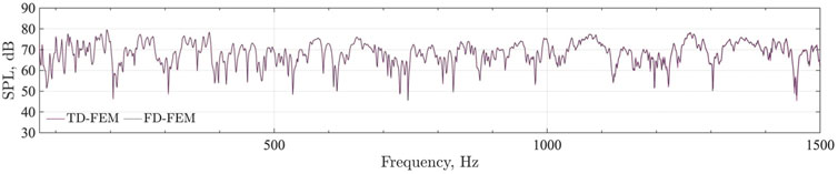
FIGURE 4. Frequency responses at R1 of TD-FEM and FD-FEM using sparse direct solver.
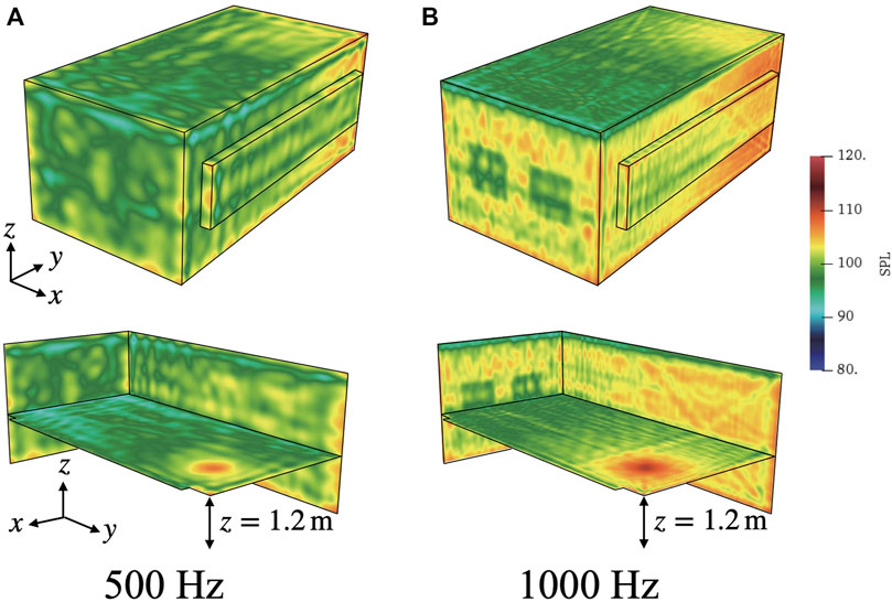
FIGURE 5. Octave band SPL distributions at 500 Hz and 1 kHz: (A) 500 Hz and (B) 1 kHz.
Figures 6A–D present comparisons of four room-acoustic parameters computed by TD-FEM and FD-FEM using PARDISO. The results presented with markers (* in TD-FEM and ◦ in FD-FEM) represent spatially averaged values against the eight receiver’s results. The error bars shown in EDT, G and C50 express their standard deviation. For T20, EDT, we also show the reverberation times calculated using the Eyring formula as a reference. Overall, TD-FEM results agree well with FD-FEM results for all room-acoustic parameters. Compared to the Eyring values, T20s values computed by FEMs are longer for all frequencies. At 1000 Hz, the FEM results show a different trend as in the Eyring values, i.e., the Eyring values decrease as frequency increases, but the FEM results do not follow the trend at 1 kHz. However, EDT values of the Eyring formula and FEMs match well at 500 Hz and 1 kHz, which indicates that the sound field in the room is still non-diffuse.
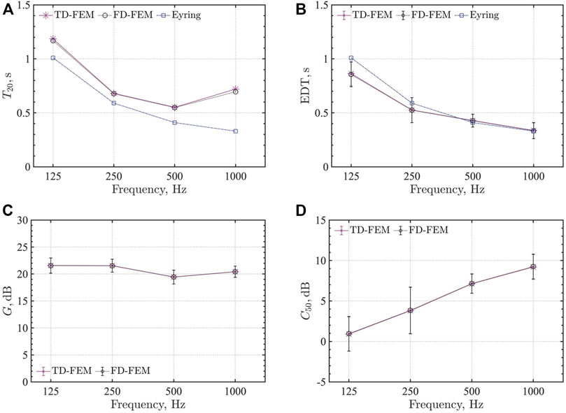
FIGURE 6. Four room-acoustic parameters of TD-FEM and FD-FEM compared using sparse direct solver: (A) T20, (B) EDT, (C) G, and (D) C50.
Table 3 lists four accuracy measures
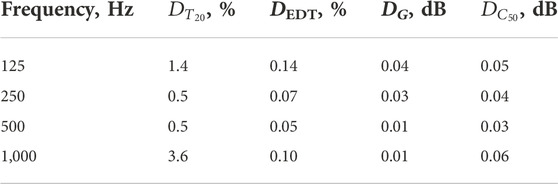
TABLE 3. Accuracy measures on four room-acoustic parameters at each frequency:
Regarding computational costs, the realistic meeting room model results showed that TD-FEM has markedly higher performance than that of FD-FEM. The computational time of TD-FEM is only 248 s when given a 0.52 GByte memory requirement when using 12 threads on OpenMP parallel computations. For the same parallel computation conditions, FD-FEM using PARDISO and CSQMOR respectively consume 78,698 s with 16.5 GByte and 39,002 s with 0.39 GByte. FD-FEM using CSQMOR is twice as fast, and with 1/42 less memory than that necessary for using PARDISO, revealing the effectiveness of using iterative solver for 3D FD-FEM at this frequency range. More importantly, TD-FEM has 157 times faster computational speed with 1.3 times larger memory requirement than FD-FEM using CSQMOR. Even in serial computation with the computational time of 2,137 s, TD-FEM is still fast: it is 18 times faster than FD-FEM using CSQMOR. This marked performance gain is attributable to its much better convergence of iterative solver in TD-FEM compared to that in FD-FEM. TD-FEM requires a mean iteration number of 5.7 per time step, but FD-FEM using CSQMOR needs mean iterations of 3985 per frequency. The total iteration of TD-FEM is 74,530, which is 1/86 of the total iteration of 6,375,544 in FD-FEM. The real-valued sparse matrix-vector product in TD-FEM further enhances the performance compared to FD-FEM with the complex-valued sparse matrix-vector product. The present result revealed that 3D TD-FEM has more attractive computational performance for room acoustics simulation than that of 3D FD-FEM. The present TD-FEM formulation can apply any type of finite elements for spatial discretization. Therefore, a similar performance gain can be expected against FD-FEM using the same finite elements. In this context, constructing higher-order TD-FEM is a subject to be addressed in future research.
4 Simulation under various sound absorber configurations
This section presents the practicality of TD-FEM for room acoustics simulation via a case study with a large-scale model having 35 million DOFs. We use the same small meeting room model in Figure 1B, but compute RIRs, which include the frequency component up to 6 kHz, under five sound absorber configurations. The five configurations include a case with no sound absorber. The remaining four use two glass wool absorbers having two characteristics and an AF absorber to control the acoustics inside the room. This demonstration will present the use of the wave-acoustics method can be a realistic selection for the room-acoustics design of small rooms.
4.1 Sound absorbers configuration
Figures 7A–E show the five sound absorber configurations C1–C5. Their details are explained below:
C1 The case with reflective interior finish: All boundary surfaces have reflective materials. Walls, the floor, the ceiling, and window frames were treated as reflective surfaces with αr = 0.08. The window and door surfaces have αr = 0.05.
C2 The case with a ceiling absorber: This case installed a GW32K absorber, the glass wool absorber with 32 kg/m3 density, to the meeting room’s ceiling. Other conditions are the same as in C1. The GW32K absorber has flow resistivity of 13,900 Pa s/m2 with 50 mm thickness.
C3 The case with a ceiling absorber and five absorbing panels on two walls: This case installed a GW32K absorber, the same as in C1, to the meeting room’s ceiling. In addition, five GW96K absorbing panels were installed on two walls of the zx plane at y = 0 and the yz plane at x = 0. Other conditions are the same as those in C1. The GW96K absorbing panels have dimensions of 0.9 m × 0.9 m × 0.025 m. Either one surface of the opposing boundary surfaces is treated with sound-absorbing material.
C4 The case with a ceiling absorber and wall absorbers on two walls: This case installed a GW96K absorber with 25 mm thickness to the meeting room’s ceiling. The GW96K absorber was installed further on two walls of the zx plane at y = 0 and yz plane at x = 0. As in C3, either one surface of the opposing boundary surfaces is treated with sound-absorbing material, but this case has a larger sound-absorbing area. Other conditions are the same as those in C1.
C5 The case with a ceiling absorber and acoustic fabric in front of a window: This case installed a GW32K absorber, the same as in C1, to the meeting room’s ceiling. An AF with the flow resistance of 462 Pa s/m and surface density of 0.12 kg/m2 was installed further with backing air cavity depth of 0.2 m in front of the windows. Other conditions are the same as those presented in C1.
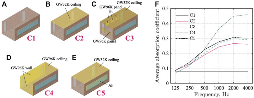
FIGURE 7. Five sound absorber configurations C1–C5 and comparison of their average absorption coefficient: (A) C1, (B) C2, (C) C3, (D) C4, (E) C5, and (F) average absorption coefficient.
Figure 7F presents a comparison of average absorption coefficient
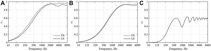
FIGURE 8. Random incidence sound absorption coefficient: (A) GW32K, (B) GW96K, (C) AF. ER and LR respectively denote the extended reaction model and local reaction model.
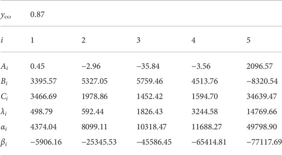
TABLE 4. Parameters y∞, Ai, Bi, Ci, λi, αi, and βi for GW32K. The parameters were fitted at 10 Hz—10 kHz.
4.2 Numerical setup
The small meeting room models with sound absorber configurations C1–C5 were spatially discretized with cubic Hex8 of 0.0125 m edge length. The resulting FE meshes have about 35 million DOFs. Their spatial resolutions are 4.6 elements per wavelength at the upper-limit frequency of 6 kHz. The RIRs were computed with a sound source signal: an impulse response of an optimized FIR filter based on the Parks–McClellan algorithm. The source signal has a flat spectrum at 70 Hz—6 kHz. The analyzed time lengths differ among cases: C1 computed RIR up to 2.5 s. For C2, C3, and C5, RIRs were computed up to 2.0 s. We computed an RIR of 1.2 s for C4. The time intervals were set to
4.3 Results
First, we explain how the reverberation time computed by TD-FEM fits the classical reverberation theory by the Eyring–Knudsen formula for cases C1 and C4 having uniform sound-absorbing surfaces in the room. We judged that those cases can better meet the reverberation theory assumption than the remaining cases. Figure 9 presents the comparison result, showing that TD-FEM results represent better agreement with the Eyring–Knudsen formula values at higher frequencies for both cases. At lower frequencies, TD-FEM results show longer reverberation times than Eyring–Knudsen formula values because of the lower diffuseness of the sound field.
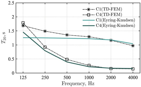
FIGURE 9. Comparison of reverberation times computed by Eyring–Knudsen formula and TD-FEM for cases C1 and C4.
Then, we discuss the characteristics of sound fields for the cases based on their average absorption coefficient magnitude relation and existing knowledge. Figures 10A–D show comparisons of the four room-acoustic parameters for cases C1–C5. In the case of C2 with a ceiling absorber, T20 does not decrease above 500 Hz despite the average absorption coefficient
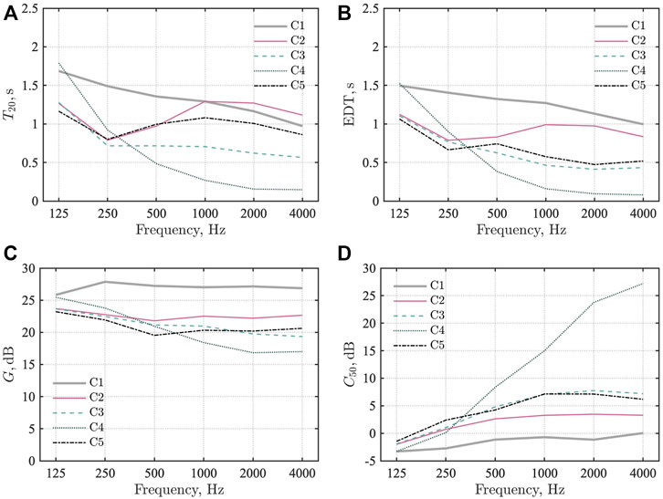
FIGURE 10. Comparison of room-acoustic parameters for cases C1–C5:(A) T20, (B) EDT, (C) G, and (D) C50.
Regarding the computational performance, the computational times were 17–20 h per unit time length for C1–C4. We required the longest time of 25 h for the case C5 having AF because C5 must use a smaller time interval according to its stability condition. The memory requirements are about 32 GByte for all cases. Note that only one node with 36 cores out of 2000 nodes on the supercomputer was used for the present computations. Also, the 32 GByte memory requirements are only 1/6 of the memory capacity of one node. Therefore, the present computations can perform on current standard workstations thoroughly. We also find the notable property of the convergence of iterative solver in TD-FEM for the sound field up to 6 kHz under various sound absorber configurations. Figure 11 presents a comparison of iteration numbers in TD-FEM among C1–C5. The iterative solver applied to TD-FEM shows a robust and stable convergence at all time steps. The convergence is markedly fast, with 4–5.2 mean iterations per time step despite those large-scale models have 35 million DOFs. Therefore, the order of iterations is
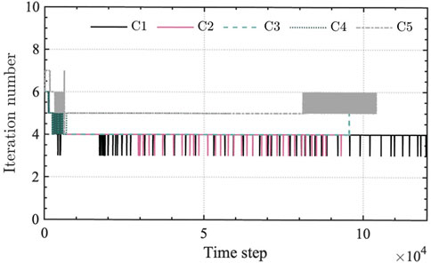
FIGURE 11. Comparison of iteration numbers among cases C1–C5.
5 Conclusion
This paper presents the applicability of a wave-based solver using the recently developed TD-FEM on 3D room-acoustic simulations of small rooms within volume on the order 10 m3. Three sound absorbers of GW, AF, and MPPGW were modeled using a frequency-dependent LR BCs and an ER model. For GW and MPPGW absorbers, the simpler LR BCs, which only consider the frequency-dependence of complex-valued specific acoustic admittance ratio, were used once confirming their consistency to ER models computed using the transfer matrix method. In the first part of this report, we explained our examination of the accuracy and efficiency of TD-FEM with the comparison of FD-FEM using two linear system solvers, PARDISO and CSQMOR. The two case studies examined herein respectively simulate RIRs of a small cubic room and a small meeting room with GW and AF porous-type sound absorbers and MPPGW resonant-type sound absorbers. The study results revealed that, compared to FD-FEMs using the two linear system solvers, TD-FEM has a high benefit for 3D small room acoustics simulation with markedly less computational time while maintaining the same accuracy as that obtained using FD-FEM. The small meeting room result showed that the computational time of FD-FEM using CSQMOR is 157 times that of TD-FEM. Moreover, the four room-acoustic parameters, T20, EDT, C50, and G, have comparable accuracies of less than the respective JND values.
Then, based on the accuracy examination with FD-FEM, the practicality of TD-FEM as a room acoustic prediction tool was demonstrated further with the large-scale acoustic simulation in the small meeting room under five sound absorber configurations up to 6 kHz. How room acoustics among the five meeting rooms change was presented by comparison of four room-acoustic parameters. The plausibility of results was demonstrated in three respects: 1) comparison of reverberation times between TD-FEM and the Eyring–Knudsen formula for cases with the most live and dead sound absorber configurations, 2) a consistency check of the results with existing knowledge related to non-diffuse rectangular rooms, and 3) a consistency check of results with the magnitude relation of average sound absorption coefficients. The computational cost results revealed that 3D TD-FEM has a remarkably appealing property for large-scale room-acoustic simulation with rapid convergence characteristics of the iterative solver. The iterative solver converged with iterations of
However, an experimental examination is still necessary to show the reliability of 3D TD-FEM on room-acoustics prediction of real rooms. We therefore show experimental examination results for real rooms with various sound absorber configurations in future studies.
Data availability statement
The original contributions presented in the study are included in the article/Supplementary Material, further inquiries can be directed to the corresponding author.
Author contributions
TO contributed to the conception and design of the study, conducted the numerical simulations, and prepared the draft of the manuscript. TY contributed to give feedback about the research design and numerical simulations, analyzed the results, and supported writing of the manuscript and coding used for the study. All authors contributed to manuscript revision, reading, and approval of the submitted version.
Funding
This work was supported in part by a Kajima Foundation Scientific Research Grant and Ono charitable Trust for Acoustics.
Conflict of interest
Author TY was employed by the company Hazama Ando Corporation.
The remaining author declares that the research was conducted in the absence of any commercial or financial relationships that could be construed as a potential conflict of interest.
Publisher’s note
All claims expressed in this article are solely those of the authors and do not necessarily represent those of their affiliated organizations, or those of the publisher, the editors and the reviewers. Any product that may be evaluated in this article, or claim that may be made by its manufacturer, is not guaranteed or endorsed by the publisher.
Supplementary material
The Supplementary Material for this article can be found online at: https://www.frontiersin.org/articles/10.3389/fbuil.2022.1006365/full#supplementary-material
References
Allard, J., and Atalla, N. (2009). “Modeling multilayered systems with porous materials using the transfer matrix method,” in Propagation of sound in porous media: Modeling sound absorbing materials (Chichester: John Wiley & Sons), 243–281.
Aretz, M., and Vorländer, M. (2014). Combined wave and ray based room acoustic simulations of audio systems in car passenger compartments, Part II: Comparison of simulations and measurements. Appl. Acoust. 76, 52–65. doi:10.1016/j.apacoust.2013.07.020
Arvidsson, E., Nilsson, E., Hagberg, D. B., and Karlsson, O. J. I. (2020). The effect on room acoustical parameters using a combination of absorbers and diffusers: An experimental study in a classroom. Acoustics 2, 505–523. doi:10.3390/acoustics2030027
Barrett, R., Berry, M., Chan, T., Demmel, J., Donato, J., Dongarra, J., et al. (1994). “Nonstationary iterative methods,” in Templates for the solution of linear systems: Building blocks for iterative methods (Philadelphia: SIAM), 14–20.
Bilbao, S., Hamilton, B., Botts, J., and Savioja, L. (2016). Finite volume time domain room acoustics simulation under general impedance boundary conditions. IEEE/ACM Trans. Audio Speech Lang. Process. 24, 161–173. doi:10.1109/TASLP.2015.2500018
Bilbao, S. (2013). Modeling of complex geometries and boundary conditions in finite difference/finite volume time domain room acoustics simulation. IEEE Trans. Audio Speech Lang. Process. 21, 1524–1533. doi:10.1109/TASL.2013.2256897
Brandão, E., Lenzi, A., and Paul, S. (2015). A review of the In Situ impedance and sound absorption measurement techniques. Acta Acustica united Acustica 101, 443–463. doi:10.3813/AAA.918840
Cardoso Soares, M., Brandão Carneiro, E., Aizik Tenenbaum, R., and Mareze, P. H. (2022). Low-frequency room acoustical simulation of a small room with BEM and complex-valued surface impedances. Appl. Acoust. 188, 108570. doi:10.1016/j.apacoust.2021.108570
Cingolani, M., Fratoni, G., Barbaresi, L., D’Orazio, D., Hamilton, B., and Garai, M. (2021). A trial acoustic improvement in a lecture hall with MPP sound absorbers and fdtd acoustic simulations. Appl. Sci. 11, 2445. doi:10.3390/app11062445
Cox, T. J., and Peter, D. (2017). Acoustic absorbers and diffusers: Theory, design and application, third edition. London: Taylor & Francis.
Cucharero, J., Hänninen, T., and Lokki, T. (2019). Influence of sound-absorbing material placement on room acoustical parameters. Acoustics 1, 644–660. doi:10.3390/acoustics1030038
Dragna, D., Pineau, P., and Blanc-Benon, P. (2015). A generalized recursive convolution method for time-domain propagation in porous media. J. Acoust. Soc. Am. 138, 1030–1042. doi:10.1121/1.4927553
Guddati, M. N., and Yue, B. (2004). Modified integration rules for reducing dispersion error in finite element methods. Comput. Methods Appl. Mech. Eng. 193, 275–287. doi:10.1016/j.cma.2003.09.010
Gumerov, N. A., and Duraiswami, R. (2021). Fast multipole accelerated boundary element methods for room acoustics. J. Acoust. Soc. Am. 150, 1707–1720. doi:10.1121/10.0006102
Gustavsen, B., and Semlyen, A. (1999). Rational approximation of frequency domain responses by vector fitting. IEEE Trans. Power Deliv. 14, 1052–1061. doi:10.1109/61.772353
Hamilton, B., and Bilbao, S. (2017). FDTD methods for 3-D room acoustics simulation with high-order accuracy in space and time. IEEE/ACM Trans. Audio Speech Lang. Process. 25, 2112–2124. doi:10.1109/TASLP.2017.2744799
Hargreaves, J. A., and Cox, T. J. (2008). A transient boundary element method model of schroeder diffuser scattering using well mouth impedance. J. Acoust. Soc. Am. 124, 2942–2951. doi:10.1121/1.2982420
Hornikx, M., Hak, C., and Wenmaekers, R. (2015). Acoustic modelling of sports halls, two case studies. J. Build. Perform. Simul. 8, 26–38. doi:10.1080/19401493.2014.959057
Hornikx, M., Krijnen, T., and van Harten, L. (2016). openPSTD: The open source pseudospectral time-domain method for acoustic propagation. Comput. Phys. Commun. 203, 298–308. doi:10.1016/j.cpc.2016.02.029
Hoshi, K., Hanyu, T., Okuzono, T., Sakagami, K., Yairi, M., Harada, S., et al. (2020). Implementation experiment of a honeycomb-backed MPP sound absorber in a meeting room. Appl. Acoust. 157, 107000. doi:10.1016/j.apacoust.2019.107000
Hughes, T. (2000). “Algorithms for hyperbolic and parabolic–hyperbolic problems,” in The finite element method linear static and dynamic finite element analysis (New York: Dover), 490–569.
ISO 10534-2 (1998). Acoustics – determination of sound absorption coefficient and impedance in impedance tubes—Part 2: Transfer-function method. Geneva: International Organization for Standardization.
ISO 3382-1 (2009). Acoustics – measurement of room acoustic parameters – Part 1: Performance spaces. Geneva: International Organization for Standardization.
ISO 9613-1 (1993). Acoustics – attenuation of sound during propagation outdoors – Part 1: Calculation of the absorption of sound by the atmosphere. Geneva: International Organization for Standardization.
Kates, J. M., and Brandewie, E. J. (2020). Adding air absorption to simulated room acoustic models. J. Acoust. Soc. Am. 148, EL408–EL413. doi:10.1121/10.0002489
Kowalczyk, K., and van Walstijn, M. (2008). Formulation of locally reacting surfaces in FDTD/K-DWM modelling of acoustic spaces. Acta Acustica united Acustica 94, 891–906. doi:10.3813/AAA.918107
Kowalczyk, K., and van Walstijn, M. (2011). Room acoustics simulation using 3-D compact explicit FDTD schemes. IEEE Trans. Audio Speech Lang. Process. 19, 34–46. doi:10.1109/TASL.2010.2045179
Labia, L., Shtrepi, L., and Astolfi, A. (2020). Improved room acoustics quality in meeting rooms: Investigation on the optimal configurations of sound-absorptive and sound-diffusive panels. Acoustics 2, 451–473. doi:10.3390/acoustics2030025
Maa, D.-Y. (1987). Microperforated-panel wideband absorbers. Noise Control Eng. J. 29, 77–84. doi:10.3397/1.2827694
Mehra, R., Raghuvanshi, N., Savioja, L., Lin, M. C., and Manocha, D. (2012). An efficient GPU-based time domain solver for the acoustic wave equation. Appl. Acoust. 73, 83–94. doi:10.1016/j.apacoust.2011.05.012
Miki, Y. (1990). Acoustical properties of porous materials – modifications of Delany–Bazley models. J. Acoust. Soc. Jpn. E. 11, 19–24. doi:10.1250/ast.11.19
Morales, N., Mehra, R., and Manocha, D. (2015). A parallel time-domain wave simulator based on rectangular decomposition for distributed memory architectures. Appl. Acoust. 97, 104–114. doi:10.1016/j.apacoust.2015.03.017
Murillo, D. M., Fazi, F. M., and Astley, J. (2019). Room acoustic simulations using the finite element method and diffuse absorption coefficients. Acta Acustica united Acustica 105, 231–239. doi:10.3813/AAA.919304
Nilsson, E. (2004). Decay processes in rooms with non-diffuse sound fields Part I: Ceiling treatment with absorbing material. Build. Acoust. 11, 39–60. doi:10.1260/1351010041217220
Okamoto, N., Tomiku, R., Otsuru, T., and Yasuda, Y. (2007). Numerical analysis of large-scale sound fields using iterative methods part II: Application of Krylov subspace methods to finite element analysis. J. Comp. Acous. 15, 473–493. doi:10.1142/S0218396X07003512
Okuzono, T., and Sakagami, K. (2015). A finite-element formulation for room acoustics simulation with microperforated panel sound absorbing structures: Verification with electro-acoustical equivalent circuit theory and wave theory. Appl. Acoust. 95, 20–26. doi:10.1016/j.apacoust.2015.02.012
Okuzono, T., and Sakagami, K. (2018). A frequency domain finite element solver for acoustic simulations of 3D rooms with microperforated panel absorbers. Appl. Acoust. 129, 1–12. doi:10.1016/j.apacoust.2017.07.008
Okuzono, T., Shimizu, N., and Sakagami, K. (2019). Predicting absorption characteristics of single-leaf permeable membrane absorbers using finite element method in a time domain. Appl. Acoust. 151, 172–182. doi:10.1016/j.apacoust.2019.03.006
Okuzono, T., Uenishi, K., and Sakagami, K. (2020). Experimental comparison of absorption characteristics of single-leaf permeable membrane absorbers with different backing air cavity designs. Noise Control Eng. J. 68, 237–245. doi:10.3397/1/376820
Okuzono, T., Yoshida, T., and Sakagami, K. (2021). Efficiency of room acoustic simulations with time-domain FEM including frequency-dependent absorbing boundary conditions: Comparison with frequency-domain FEM. Appl. Acoust. 182, 108212. doi:10.1016/j.apacoust.2021.108212
Otsuru, T., Tomiku, R., Okamoto, N., and Ichikawa, Y. (2000). “Accuracy of finite element sound field analysis of an irregular shaped reverberation room,” in Proceedings of the seventh international congress on acoustics (Garmisch-Partenkirchen, 2093–2100.
Otsuru, T., Tomiku, R., Toyomasu, M., and Takahashi, Y. (2001). “Finite element sound field analysis of rooms in built environment,” in Proceedings of the eighth international congress on acoustics (Hong Kong, 765–772.
Pind, F., Engsig-Karup, A. P., Jeong, C.-H., Hesthaven, J. S., Mejling, M. S., and Strømann-Andersen, J. (2019). Time domain room acoustic simulations using the spectral element method. J. Acoust. Soc. Am. 145, 3299–3310. doi:10.1121/1.5109396
Pind, F., Jeong, C.-H., Engsig-Karup, A. P., Hesthaven, J. S., and Strømann-Andersen, J. (2020). Time-domain room acoustic simulations with extended-reacting porous absorbers using the discontinuous galerkin method. J. Acoust. Soc. Am. 148, 2851–2863. doi:10.1121/10.0002448
Pind, F., Jeong, C.-H., Hesthaven, J. S., Engsig-Karup, A. P., and Strømann-Andersen, J. (2021). A phenomenological extended-reaction boundary model for time-domain wave-based acoustic simulations under sparse reflection conditions using a wave splitting method. Appl. Acoust. 172, 107596. doi:10.1016/j.apacoust.2020.107596
Rabisse, K., Ducourneau, J., Faiz, A., and Trompette, N. (2019). Numerical modelling of sound propagation in rooms bounded by walls with rectangular-shaped irregularities and frequency-dependent impedance. J. Sound Vib. 440, 291–314. doi:10.1016/j.jsv.2018.08.059
Sakagami, K., Morimoto, M., and Yairi, M. (2005). A note on the effect of vibration of a microperforated panel on its sound absorption characteristics. Acoust. Sci. Technol. 26, 204–207. doi:10.1250/ast.26.204
Sakamoto, S., Nagatomo, H., Ushiyama, A., and Tachibana, H. (2008). Calculation of impulse responses and acoustic parameters in a hall by the finite-difference time-domain method. Acoust. Sci. Technol. 29, 256–265. doi:10.1250/ast.29.256
Sakamoto, N., Otsuru, T., Tomiku, R., and Yamauchi, S. (2018). Reproducibility of sound absorption and surface impedance of materials measured in a reverberation room using ensemble averaging technique with a pressure-velocity sensor and improved calibration. Appl. Acoust. 142, 87–94. doi:10.1016/j.apacoust.2018.08.009
Sakamoto, S. (2007). Phase-error analysis of high-order finite difference time domain scheme and its influence on calculation results of impulse response in closed sound field. Acoust. Sci. Technol. 28, 295–309. doi:10.1250/ast.28.295
Sakuma, T., Sakamoto, S., and Otsuru, T. (2014). Computational simulation in architectural and environmental acoustics: Methods and applications of wave-based computation. Tokyo: Springer Japan.
Savioja, L., and Svensson, U. P. (2015). Overview of geometrical room acoustic modeling techniques. J. Acoust. Soc. Am. 138, 708–730. doi:10.1121/1.4926438
Simonaho, S-P., Lähivaara, T., and Huttunen, T. (2012). Modeling of acoustic wave propagation in time-domain using the discontinuous galerkin method: A comparison with measurements. Appl. Acoust. 73, 173–183. doi:10.1016/j.apacoust.2011.08.001
Sugahara, A., Lee, H., Sakamoto, S., and Takeoka, S. (2019). Measurements of acoustic impedance of porous materials using a parametric loudspeaker with phononic crystals and phase-cancellation method. Appl. Acoust. 152, 54–62. doi:10.1016/j.apacoust.2019.03.019
Toyoda, M., and Eto, D. (2019). Prediction of microperforated panel absorbers using the finite-difference time-domain method. Wave Motion 86, 110–124. doi:10.1016/j.wavemoti.2019.01.006
Toyoda, M., and Sakayoshi, Y. (2021). Filter and correction for a hybrid sound field analysis of geometrical and wave-based acoustics. Acoust. Sci. Technol. 42, E2111–E2180. doi:10.1250/ast.42.170
Troian, R., Dragna, D., Bailly, C., and Galland, M.-A. (2017). Broadband liner impedance eduction for multimodal acoustic propagation in the presence of a mean flow. J. Sound Vib. 392, 200–216. doi:10.1016/j.jsv.2016.10.014
Vorländer, M. (2013). Computer simulations in room acoustics: Concepts and uncertainties. J. Acoust. Soc. Am. 133, 1203–1213. doi:10.1121/1.4788978
Wang, H., and Hornikx, M. (2020). Time-domain impedance boundary condition modeling with the discontinuous galerkin method for room acoustics simulations. J. Acoust. Soc. Am. 147, 2534–2546. doi:10.1121/10.0001128
Wang, H., Sihar, I., Muñoz, R. P., and Hornikx, M. (2019). Room acoustics modelling in the time-domain with the nodal discontinuous galerkin method. J. Acoust. Soc. Am. 145, 2650–2663. doi:10.1121/1.5096154
Yasuda, Y., Ueno, S., Kadota, M., and Sekine, H. (2016). Applicability of locally reacting boundary conditions to porous material layer backed by rigid wall: Wave-based numerical study in non-diffuse sound field with unevenly distributed sound absorbing surfaces. Appl. Acoust. 113, 45–57. doi:10.1016/j.apacoust.2016.06.006
Yasuda, Y., Saito, K., and Sekine, H. (2020). Effects of the convergence tolerance of iterative methods used in the boundary element method on the calculation results of sound fields in rooms. Appl. Acoust. 157, 106997. doi:10.1016/j.apacoust.2019.08.003
Yatabe, K., and Sugahara, A. (2022). Convex-optimization-based post-processing for computing room impulse response by frequency-domain fem. Appl. Acoust. 199, 108988. doi:10.1016/j.apacoust.2022.108988
Yoshida, T., Okuzono, T., and Sakagami, K. (2020). Time-domain finite element formulation of porous sound absorbers based on an equivalent fluid model. Acoust. Sci. Technol. 41, 837–840. doi:10.1250/ast.41.837
Yoshida, T., Okuzono, T., and Sakagami, K. (2022). A parallel dissipation-free and dispersion-optimized explicit time-domain FEM for large-scale room acoustics simulation. Buildings 12, 105. doi:10.3390/buildings12020105
Yue, B., and Guddati, M. N. (2005). Dispersion-reducing finite elements for transient acoustics. J. Acoust. Soc. Am. 118, 2132–2141. doi:10.1121/1.2011149
Zhang, J., and Dai, H. (2015). A new quasi-minimal residual method based on a biconjugate a-orthonormalization procedure and coupled two-term recurrences. Numer. Algorithms 70, 875–896. doi:10.1007/s11075-015-9978-5
Zhao, J., Chen, Z., Bao, M., Lee, H., and Sakamoto, S. (2019). Two-dimensional finite-difference time-domain analysis of sound propagation in rigid-frame porous material based on equivalent fluid model. Appl. Acoust. 146, 204–212. doi:10.1016/j.apacoust.2018.11.004
Nomenclature
Boundary conditions
ER Extended-reaction
LR Local-reaction
Numerical methods
ADE Auxiliary differential equation
ARD Adaptive rectangular decomposition
BEM Boundary element method
CG Conjugate gradient
CSQMOR Complex symmetric quasi-minimal residual method based on coupled two-term biconjugate A-orthonormalization procedure
DG-FEM Discontinuous Galerkin FEM
FD-FEM Frequency-domain FEM
FDTD Finite-difference time-domain
FEM Finite element method
FVTD Finite-volume time-domain
PSTD Pseudospectral time-domain
TD-BEM Time-domain BEM
TD-FEM Time-domain FEM
TD-SEM Time-domain spectral element method
Other symbols
FD Frequency-domain
JND Just noticeable difference
RIR Room impulse response
TD Time-domain
Sound absorbers
AF Acoustic fabric curtain
GW Glass wool
MPP Microperforated panel
MPPGW MPP absorber backed by GW
Keywords: frequency-domain finite element method, room acoustics simulation, small-room acoustics, acoustic design, time-domain finite element method, wave-based method
Citation: Okuzono T and Yoshida T (2022) High potential of small-room acoustic modeling with 3D time-domain finite element method. Front. Built Environ. 8:1006365. doi: 10.3389/fbuil.2022.1006365
Received: 29 July 2022; Accepted: 22 November 2022;
Published: 02 December 2022.
Edited by:
Arianna Astolfi, Politecnico di Torino, ItalyReviewed by:
Tapio Lokki, Aalto University, FinlandReza Soleimanpour, Australian College of Kuwait, Kuwait
Jonathan Hargreaves, University of Salford, United Kingdom
Copyright © 2022 Okuzono and Yoshida. This is an open-access article distributed under the terms of the Creative Commons Attribution License (CC BY). The use, distribution or reproduction in other forums is permitted, provided the original author(s) and the copyright owner(s) are credited and that the original publication in this journal is cited, in accordance with accepted academic practice. No use, distribution or reproduction is permitted which does not comply with these terms.
*Correspondence: Takeshi Okuzono, b2t1em9ub0Bwb3J0LmtvYmUtdS5hYy5qcA==