Spatial clustering of waste reuse in a circular economy: A spatial autocorrelation analysis on locations of waste reuse in the Netherlands using global and local Moran’s I

In recent years, implementing a circular economy in cities has been considered by policy makers as a potential solution for achieving sustainability. Existing literature on circular cities is mainly focused on two perspectives: urban governance and urban metabolism. Both these perspectives, to some extent, miss an understanding of space. A spatial perspective is important because circular activities, such as the recycling, reuse, or storage of materials, require space and have a location. It is therefore useful to understand where circular activities are located, and how they are affected by their location and surrounding geography. This study therefore aims to understand the existing state of waste reuse activities in the Netherlands from a spatial perspective, by analyzing the degree, scale, and locations of spatial clusters of waste reuse. This was done by measuring the spatial autocorrelation of waste reuse locations using global and local Moran’s I, with waste reuse data from the national waste registry of the Netherlands. The analysis was done for 10 material types: minerals, plastic, wood and paper, fertilizer, food, machinery and electronics, metal, mixed construction materials, glass, and textile. It was found that all materials except for glass and textiles formed spatial clusters. By varying the grid cell sizes used for data aggregation, it was found that different materials had different “best fit” cell sizes where spatial clustering was the strongest. The best fit cell size is ∼7 km for materials associated with construction and agricultural industries, and ∼20–25 km for plastic and metals.The best fit cell sizes indicate the average distance of companies from each other within clusters, and suggest a suitable spatial resolution at which the material can be understood. Hotspot maps were also produced for each material to show where reuse activities are most spatially concentrated.

Introduction

Our current “take-make-waste” or linear economy of production, where materials are extracted, used, and discarded as waste, is unsustainable. There is a pressing need to transition to more sustainable socio-technical systems that address environmental problems, such as resource depletion and excessive land use; as well as economic problems, such as supply risk and flawed incentive structures (Geissdoerfer et al., 2017). Since 2015, transitioning to a circular economy (CE) has been proposed by policy makers in the European Commission as a potential solution (European Commission, 2020). In the Netherlands, companies and households produce over 43 million tonnes of waste per year, including waste materials such as food waste, packaging, iron, paper, plastics, glass, chemical waste, and construction waste (Statistics Netherlands 2020). As part of its circular economy strategy, the Netherlands aims to increase waste reuse for the production of goods, in order to reduce the need to extract or import scarce raw materials, reducing pressure on the environment (Hanemaaijer et al., 2021).

Although there is no consensus on its definition (Kirchherr et al., 2017), a commonly adopted notion of CE is keeping materials and products performing at their highest application level for as long as possible, while reducing environmental impacts and being aware of environmental trade-offs. CE has also been put forward as an alternative economic paradigm that stays within planetary boundaries and is socially just (Marin et al., 2020). The study of circular economy was popularized by the fields of industrial ecology, industrial design, and business management; and examined the circularity of materials, products, and companies (Bocken et al., 2016; Kalmykova et al., 2018; Bakker et al., 2019; Hollander et al., 2017).

Recently, there have been growing efforts to look beyond products to larger spatial scales—to buildings, cities, regions, and beyond; introducing the question of what is a suitable spatial scale at which to organize and model material flow and distribution. Much of these efforts fall under the topic of “circular cities,” and take the perspectives of urban governance, which studies the circularity of a city’s policies and stakeholders (Prendeville et al., 2018; Amenta et al., 2019; Williams 2019a); and urban metabolism, which studies the material, water, or energy flows of cities or regions (Kennedy et al., 2007; Broto et al., 2012; Dijst et al., 2018).

The study of circular cities requires a spatial or geographical perspective. For cities, transitioning to a circular economy requires the introduction of circular (industrial) activities into the region, such as recycling, remanufacturing, storage, and (reverse) logistics; which are affected by spatial factors such as proximity to materials, clients, suppliers, and other companies. Because of this, scholars have started to recognize the importance of adding a geographical or spatial perspective to the study of circular cities and regions (Stephan and Athanassiadis 2017; Wandl 2020; Van den Berghe and Verhagen 2021; Sprecher et al., 2021; Furlan et al., 2022). The development of this perspective is still at an early stage, and the increasing accessibility and quality of spatial material flow data presents new possibilities. Accessible spatial material data and spatial analysis tools could provide a greatly enhanced ability to generate insights for circular economy at the regional scale. However, as more have access to these powerful tools, it is also more important to identify the limitations of spatial data analysis.

This paper aims to add a spatial perspective to the study of circular economy by analyzing the spatial clustering of existing waste reuse activities in the Netherlands. This study answers the research question: “How does analyzing the spatial clustering and hotspots of waste reuse locations generate insights for the circular economy, and what are the limitations of these insights?” Spatial autocorrelation methods, global and local Moran’s I, were used to analyze the spatial clustering of the waste reuse locations in the Netherlands for minerals, mixed construction materials, food, fertilizer, metal, plastic, wood and paper, and machinery and electronics.

A key finding was made from varying the grid cell sizes used to aggregate the reuse location data. It was found that each material had a “best fit” cell size that optimized the trade-offs between cell sizes too large and too small. Materials associated with the construction and agriculture industry (minerals, mixed construction materials, food, and fertilizer) had a best fitting cell size of 7 km, wood and paper of 15 km, metals and plastics of ∼20–25 km, while machinery and electronics had no clear best fit cell size. Additionally, local spatial autocorrelation results were used to generate hotspot maps for each material, which indicated locations with a significantly high rate of waste reuse. Together, the best fit cell size and hotspot maps for each material could provide insights on which spatial scale to analyze the material, which level of governance (municipal, provincial) to write policy influencing the material, as well as other spatial attributes such as the material’s relationship to urban areas and level of centralization.

Literature review

While earlier studies on CE focused on the circularity of materials, products, and companies; researchers have started exploring circularity at larger geographical scales—expanding from the product scale to neighborhoods (Codoban and Kennedy 2008), cities (Kennedy et al., 2007), countries (Tanikawa et al., 2015), and even the entire globe (Graedel et al., 2019).

Space, people, and flow of circular cities and regions

The larger scale perspectives on material flows in a circular economy can be categorized in three perspectives, following the environmental planning framework of (Tjallingii 1996): space, people, and flows. While the following paragraphs explains these three perspectives separately, it is important to note that an integrated perspective is required for a truly meaningful understanding of circular cities and regions.

The spatial perspective, within the disciplines of urban design and planning, investigates how land use, planning, and zoning strategies affect circular activity and material flows in regions. Strategies can come in the form of developing circular infrastructure, such as adequate space for storage of materials and (circular) industrial activity, and a well functioning reverse logistics network. This could facilitate the circular flow of resources, helping to reduce the city’s intensive resource use and to tackle urban waste streams (Arciniegas et al., 2019; Williams 2019b; Wandl 2020).

The people perspective, within the urban governance context, investigates how municipalities and policy makers implement a circular economy at a city, provincial, or country level. Research from this topic involves examining policies, regulations, and strategies to understand how they facilitate, hinder, or change waste-to-resource flows; as well as listing out societal barriers for regions attempting to implement a circular economy (Prendeville et al., 2018; Amenta et al., 2019; Bolger and Doyon 2019; Van den Berghe and Vos 2019).

The flows perspective, within the field of urban metabolism, describes the flow of resources through a region be it a city, province, or country, in particular the movement and consumption of materials, energy, and water (Brunner 2007; Kennedy et al., 2007; Broto et al., 2012; Dijst et al., 2018). It also investigates how various strategies can contribute to reducing the resource use of regions, by reducing the overall consumption of raw materials, and using industrial processes to turn waste into a resource. Our study, which analyzes the locations of waste reuse in the Netherlands, attempts to contribute to the space and flows perspective of circular regions.

Urban metabolism

The flows perspective on circular regions stems from the broader and more established field of urban metabolism, which studies “the sum total of the technical and socio-economic processes that occur in cities, resulting in growth, production of energy and elimination of waste” (Kennedy et al., 2007). Literature on urban metabolism began in the 1960s, with a seminal study by (Wolman 1965), in which national data on water, food, fuel use, and production rates of waste per capita was used to estimate the flow rates of a hypothetical American city of one million people.

Urban metabolism studies examine a wide variety of flows in a city or region, such as water, materials, or nutrients, in terms of mass fluxes, usually in kg or tons (Kennedy and Bunje 2011). While most urban metabolism literature illustrate the input of resources and output of waste, some papers examine cyclical urban metabolism or waste metabolism, where waste produced by a region is considered as a secondary resource or input for the city. Urban metabolism studies on waste recognize that, while products are produced from resource flow pathways, waste is processed by waste treatment and recycling pathways (Zhang 2013).

In its early stages, urban metabolism treated cities and regions as a system boundary for material flow analysis, rather than a topic of study, also known as a “black box model” (Song et al., 2018). The first studies in urban metabolism were accounting exercises to calculate the total input, stock, and output of water, materials, nutrients, and waste of specific cities. There was less discussion on how the spatial aspects of the city (e.g., density, land use, proximity, and accessibility) affected the location of these flows. As urban metabolism developed, so did its approach to space, resulting in a variety of spatial approaches (Dijst et al., 2018). This includes mapping (geo-visualization) of stocks and flows, calculating eco-footprint of cities, incorporating insights into urban design and planning, and spatial modeling.

Mapping of stocks includes visualization for urban mining purposes, such as construction material stock mapping (Tanikawa et al., 2015; Stephan and Athanassiadis 2017; Sprecher et al., 2021); while mapping of flows include visualization of material flows (Furlan et al., 2022; Sileryte et al., 2022), and activity based spatial material flow analysis (Dijst et al., 2018).

The study of ecological footprint of cities determines the amount of land required to provide a city with its resources and process its waste. Studies of this nature have been conducted for Vancouver, Santiago de Chile, Cardiff, and cities of the Baltic region of Europe (Kennedy et al., 2007). The past decade has seen many more similar studies, mostly focusing on the so-called megapolis—metropolitan areas with a population exceeding ten million (Moore et al., 2013; Geng et al., 2014).

Spatial modeling (or spatial statistics, spatial econometrics) combines statistics and geometry to create statistical spatial models of material flows, allowing researchers to make predictions for future scenarios and support spatial policy decisions (Dijst et al., 2018). Urban resource demands are simulated using activity-based modeling by (Keirstead and Sivakumar 2012; Zhang 2013; Li and Kwan 2018). Other researchers have considered the interactions between an urban metabolism and the spatial distribution of land use and cover types (Zhang 2013).

Spatial clustering and circular regions

One potentially important aspect of geographically explicit urban metabolism is the study of spatial clustering. While there are not many spatial clustering studies on waste reuse locations, statistical tools for studying spatial clustering have been applied to many topics—from the clustering of molecules and atoms in materials studied by material scientists, to the clustering of black holes and planets studied by astrophysicists. Literature relevant to urban metabolism are studies examining spatial clustering from the perspective of waste management, urban mining, and company location.

Literature studying spatial clustering from a waste management perspective studies hot spots of waste production in order to inform waste management, recovery, and policy (Antczak 2020; Cheniti et al., 2021). Similar methods are also used to identify hot spot areas with high concentrations of hazardous materials in air, soil, or water; in order to minimize negative environmental impacts of pollution (Rawlins et al., 2005; Huo et al., 2012; Zhao et al., 2014).

Literature on spatial clustering from an urban mining perspective identifies geographical clusters within a region where secondary materials (such as precious metals from e-waste, or building materials) can be extracted in the future (Zhu 2014; Zhang et al., 2019). This is done through material stock analysis, such as estimating the location of construction material stocks by aggregating cadaster data, which is a comprehensive recording of real estate in a country, including information on building function, age, and height (Sprecher et al., 2021; Verhagen et al., 2021).

Literature on the spatial clustering of companies stems from a spatial econometrics perspective, which uses spatial statistical methods to verify hypotheses on theories of company location, spatial agglomeration, and economies of scale. These studies identify industry clusters in order to explain and inform regional economic development, such as infrastructure (including waste infrastructure), policy instruments, environmental laws (Baptista and Swann 1999; Malmberg and Maskell 2002; López and Antonio 2017; Sunny and Cheng 2019; Hassan et al., 2020).

Research gaps

In circular economy research, the spatial study of material flows at the city or regional scale is still in its infancy. This could be because the concept of circular economy stemmed from the fields of industrial ecology, business and product design, which include the study of “people,” such as management and business models for circular companies; and of “flows,” such as secondary materials and reuse methods for circular production, but has less focus on issues related to space. Another reason could be the lack of data on material stocks and flows, as well as the all encompassing and complex nature of materials, making it difficult to define the scope of research. While other flows such as energy and transportation can be easily recorded by a centralized provider and made publicly available via census data; data on material flows is harder to collect—there is no centralized provider of “materials,” nor is there a straightforward way to automatically record data on material flows (Zhu 2014).

In urban metabolism research, most studies are also not spatially explicit. The majority of existing literature understands the metabolism of regions as a whole, without zooming in to examine the geographical locations of flows within the region. Of the urban metabolism studies that are spatially explicit, few studies have gone beyond geo-visualization to use spatial statistical methods (Verhagen et al., 2021). While the location of clusters or hotspots can be roughly identified by interpreting the maps visually, there is rarely spatial statistical work describing objectively how strongly materials are clustered, and where these clusters are. This could be due to the lack of detailed location data on materials, as well as the lack of accessible spatial analysis tools in the past. While spatial data on material flows may be available at the country scale through input-output tables, there is limited availability of material data at the regional, urban, or neighborhood level (Zhu 2014).

In spatial clustering research, studies have been conducted for other disciplines and topics, locating clusters of companies, pollutants, material stock, even waste production. However, the authors have not found any studies on locations of waste reuse. This is again due to lack of data. Since spatial clustering analysis has not been conducted on locations of waste reuse before, more investigation is needed for the potential insights and limitations of the spatial clustering results, especially on how (or whether) these results could provide advice for circular regional development.

Our research therefore applies existing spatial analysis methods to new data (locations of waste reuse) that were previously unavailable to researchers, in order to explore how our results could contribute to circular regional development. In terms of methodological contributions, our paper yields new intuition on the choice of a grid size when aggregating spatial values and its consequences on spatial clustering.

Research aim and questions

The aim of this research is to explore how using statistical methods to analyze the spatial clustering of waste reuse in the Netherlands could provide insights for circular regional development, in order to bridge the gap between urban design and urban metabolism.

The research question is therefore: What insights and caveats can be derived from spatial clustering analysis of waste reuse locations? The sub-research questions are:

What is the degree, scale, and location of spatial clustering of waste reuse locations in the Netherlands?

What are the potential insights and caveats of identifying hotspot locations of waste reuse locations in the Netherlands?

Methodology

This research uses statistical methods to analyze the spatial clustering of waste reuse locations in the Netherlands. Three aspects of spatial clustering will be measured: how strongly waste reuse activities are clustered across the country, the spatial scale at which reuse activities are most strongly clustered, and the hotspots of waste reuse clusters. Global and local Moran’s I, one of the most commonly used and accepted methods for analyzing spatial clustering in the fields of spatial econometrics and location science, will be used to understand the three aspects of spatial clustering mentioned above (Getis and Ord 1992; Anselin 1995).

Waste reuse data from the Dutch National Waste Registry was utilized. The data was plotted onto a map of the Netherlands as point data, then categorized by material types. For each material type, the following steps were conducted:

The waste reuse point data was aggregated into 50 grids, with cell sizes varying from 1 to 50 km.

Global Moran’s I was calculated for each of the 50 grids (cell sizes: 1–50 km) to measure the degree of spatial clustering for each cell size.

A trendline was plotted with cell size on the x-axis and degree of clustering on the y-axis, in order to identify the cell size at which clustering is the strongest.

Local Moran’s I was used to map out the hotspots of waste reuse—locations where the amount of waste reuse is significantly high.

The steps above are summarized in Figure 1. The details of the materials and methods are further elaborated in the sub-sections below.

FIGURE 1

FIGURE 1. Flowchart of materials and methods used, created by authors.

Data preparation

This study utilized data from the Dutch National Waste Registry (Landelijk Meldpunt Afvalstoffen, LMA), which records all waste flows in the Netherlands that are processed by waste management companies, and includes information on the location of waste producers, processors, and secondary resource receivers; as well as the weight and material type of the waste produced. This study focuses on the location of “first receivers” (“eerste afnemers” in Dutch), which are non-waste management companies that receive processed waste as a secondary resource from waste processors. The locations “first receivers” were chosen because they most resembled locations of waste reuse. The locations of waste reuse were then aggregated onto a gridded map of the Netherlands (Figure 2), with each grid cell representing the sum weight of waste reused for the data points located within the cell.

FIGURE 2

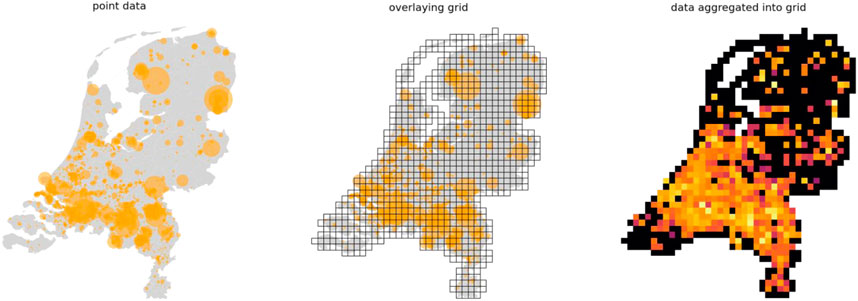
FIGURE 2. Aggregating point data to polygon data by overlaying grid, figure created by authors.

For each grid cell, the amount of waste reused was further categorized by material type. The LMA dataset represents the material type of each waste flow using either the European waste code (EWC) or the combined nomenclature code (CN). However, the categories were difficult to interpret because the categories of the two code types (EWC and GN) did not match well. In order to create more meaningful categorizations, the waste flows were re-categorized using keywords.

Finally, some flows in the LMA dataset were deemed as “invalid” because the location of the first receiver in the dataset was either a temporary storage location, or did not represent the true location of reuse, but rather the location of the headquarters of the first receiver company. These “invalid” flows were removed with consultation with waste experts from the Rijkswaterstaat (government agency for public works and water management).

Global Moran’s I—degree and scale of spatial clustering

Global spatial autocorrelation was used to understand the strength of spatial clustering of waste reuse locations in the Netherlands. Spatial autocorrelation is a term used to describe the presence of systematic spatial variation in a variable. A positive spatial autocorrelation of a dataset would mean that areas closer together are more similar than areas further apart. While there are multiple methods of measuring global spatial autocorrelation, this study has chosen Moran’s I (Getis and Ord 1992) as the measurement method. This is because it is one of the most commonly known spatial autocorrelation methods used in exploratory spatial data analysis, popularized by interface-based GIS (geographical information systems) tools like GeoDa and ArcGIS. This study therefore aims to focus on Moran’s I to illustrate its potentials and pitfalls, while leaving other spatial autocorrelation methods to future studies. For this study, Global Moran’s I was used to indicate the degree of spatial clustering for the materials in the LMA dataset, as well as the statistical significance of this clustering. Moran’s I values can vary from −1 to 1. A value approaching 1 indicates strong spatial clustering, −1 indicates strong spatial dispersion, and 0 indicates the absence of large clusters (Figure 3).

FIGURE 3

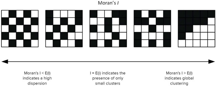
FIGURE 3. Illustration of how map clustering affects Moran’s I score. Image adapted from (Kirkegaard 2015).

The global Moran’s I of a spatial random variable X is:

$I = \frac{n}{W}\frac{{\displaystyle \sum _{i=1}^n{\displaystyle \sum _{i=1}^n{W}_{ij}\left(X_i-\overline{X}\right)\left(X_j-\overline{X}\right)}}}{{\displaystyle \sum _{i=1}^n{\left(X_i-\overline{X}\right)}^2}}$

Where $n$ is the number of spatial units indexed by $i$ and $j$; $X$ is the variable of interest (in our case, kg of materials reused); $\underset{¯}{X}$ is the mean of $x$; $W_{ij}$ is a queen weight matrix of spatial weights with zeroes on the diagonal, where $W_{ij}=1$ if cells i and j share an edge or a vertice; and $W$ is the sum of $W_{ij}$. A p-value was also calculated for the global Moran’s I values for each material using a Monte Carlo method. Further explanation can be found in the Supplementary Materials.

Aggregating the waste reuse data at different scales produced varying results for spatial clustering. This is a common phenomenon seen in geography, and is known as the modifiable areal unit problem (MAUP) (Openshaw 1983). The MAUP is a source of statistical bias that comes from aggregating point data into polygons. The bias takes two main forms: the scale effect, and the zone effect. Figure 4 below shows how the representation of point location data can be significantly changed by changing the scale (Figure 4A) and zone (Figure 4B) of aggregation.

FIGURE 4

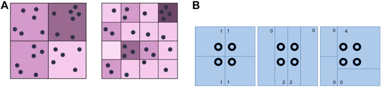
FIGURE 4. (A) Scale effect of the modifiable areal unit problem (GIS Geography 2022). (B) Zone effect of the modifiable areal unit problem (GIS Lounge 2018).

In order to address the MAUP scale effect, each material type in the dataset was aggregated to grids of different cell sizes, from 1–50 km. To address the zone effect, each grid was shifted randomly four times. For each grid variation (in scale and position), the Global Moran’s I and p-value [of the test E(I) = 0] were calculated. The resulting 5 Moran’s I values (1 original + 4 shifts) at each cell size were then plotted onto a graph with Moran’s I on the y-axis and cell size on the x-axis. A LOWESS (locally weighted scatterplot smoothing) trendline was then used to estimate the cell size which results in the strongest spatial clustering, see Figure 5 below.

FIGURE 5

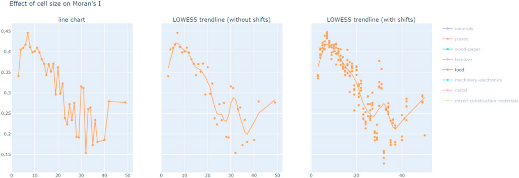
FIGURE 5. Creating the LOWESS trendline that shows cell sizes with strongest spatial clustering for food reuse. Charts created by authors.

The cell size which results in the strongest spatial clustering can be identified by varying the cell size for each material. This is important because spatial clustering for different materials can occur at different scales—from neighborhoods, to cities, to provinces. With this method of varying cell sizes for each material, the different spatial scales of different materials can be understood and compared.

Usually, the relatively large number cell sizes in this study would require multiple comparison corrections to account for false positives in order to establish statistical significance. However, we argue that this is irrelevant in this study. The theoretical aim of this study is to test an infinite number of cell sizes between a minimum and maximum (1–50 km), whereas multiple comparison corrections account for a finite amount of hypotheses. For a more detailed explanation, refer to the Supplementary Materials.

Local Moran’s I—locations of spatial clusters

Finally, local spatial autocorrelation (Anselin 1995) was used to identify the locations of clusters for each material type. Unlike global spatial autocorrelation, local spatial autocorrelation focuses on the relationships between each observation (each grid cell) and its neighbors, rather than providing a single-number summary for the whole map. While global Moran’s I accesses the strength of clustering of a map as a whole, local Moran’s I identifies the location of clusters on the map. The formula for local Moran’s I is similar to its “global” counterpart; the only difference is that, while the global Moran’s I formula iterates through all pairs of polygons, the local Moran’s I formula only iterates through the neighbors of one polygon. The formula for local Moran’s I is shown below.

The local Moran’s I of a spatial random variable $\mathrm{X}$ is:

$I_i= \frac{X_i-\overline{X}}{S_i^2} {\displaystyle \sum _{j=1, j\ne i}^n{W}_{ij}\left(X_j-\overline{X}\right)}$

Where $X_i$ is an attribute for feature $i$, $\overline{X}$ is the mean of the corresponding attribute, $W_{ij}$ is the spatial weight between feature $i$ and $j$, and:

$S_i^2= \frac{ {\displaystyle \sum _{j=1, j\ne i}^n{\left(X_j-\overline{X}\right)}^2}}{n - 1}$

With $n$ equating to the total number of features.

The significance of a local Moran’s I value is determined in the same fashion as global Moran’s I, except that the permutation is carried out for each observation in turn, resulting in a p-value for every polygon on the map (as opposed to one p-value for the whole map).

In order to identify the types of clusters, local Moran’s I calculations are combined with the Moran scatter plot. This plots, for each polygon (such as a grid cell of a map), its value on the x-axis (such as kg waste reused), and the average value of its neighbors on the y-axis (also known as spatial lag). By separating the Moran’s scatter plot into four quadrants and calculating each polygon’s significance, we can define locations as spatial clusters of either high values surrounded by high values (hotspots) or low values surrounded by low values (cold spots); as well as spatial outliers that are low values surrounded by high values (doughnuts) or high values surrounded by low values (diamonds). An example of a Moran’s scatter plot and its four quadrants is shown in Figure 6 below.

FIGURE 6

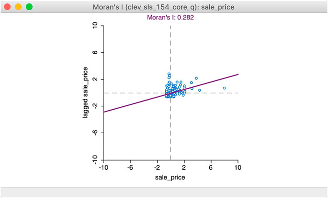
FIGURE 6. Moran’s I scatter plot (Anselin, 2020).

Results

Global Moran’s I—degree and scale of spatial clustering

By mapping waste reuse locations on a gridded map of the Netherlands, varying the cell sizes of the grids, and calculating the global Moran’s I value for each of these maps, the strength and scale of spatial clustering for waste reuse for the different material types can be identified. For more details on this process, please refer to the materials and methods section. For each material, the Moran’s I value for each cell size was compared to a random case, where the same values were used but the coordinates were randomly shuffled. The resulting charts and more detailed explanation can be found in the Supplementary Materials. The resulting line charts (Figure 7) below shows how varying cell sizes for aggregation affects the degree of spatial clustering (Moran’s I) and statistical significance (p-value) of each material in the waste reuse dataset. For both plots below, the x-axis represents the cell sizes of the grid map used to aggregate the data, varying from 1 to 50 km. For Figure 6A, the y-axis represents the global Moran’s I value, while for Figure 6B, it represents the p-value. As seen in the Figures below, the majority of materials and cell sizes resulted in p-value ≤ 0.05, with the exception of the materials glass and textile.

FIGURE 7

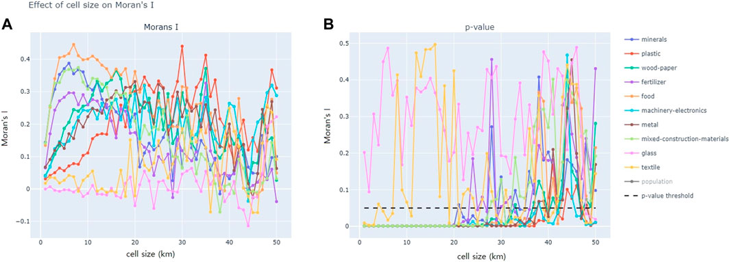
FIGURE 7. (A) Effect of cell size on Moran’s I value; (B) effect of cell size on p-value. Charts created by authors.

Figure 8 below shows how the strength of clustering (y-axis, represented by global Moran’s I) is affected by cell size used for aggregation (x-axis), after statistically insignificant cell sizes and materials have been eliminated.

FIGURE 8

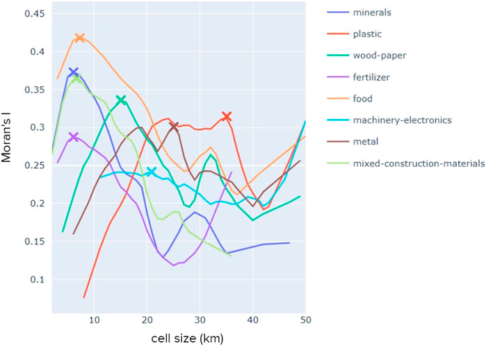
FIGURE 8. Effect of cell size on Moran’s I value for all materials, created by authors.

As seen in Figure 7, the trendline for most materials forms a peak, meaning that most materials have an “best fit” aggregation cell size where spatial clustering is the most prominent. For each material in the LMA dataset, the “best fit” cell size, as well as the global Moran’s I value and p-value for that cell size, is summarized in Table 1 below.

TABLE 1

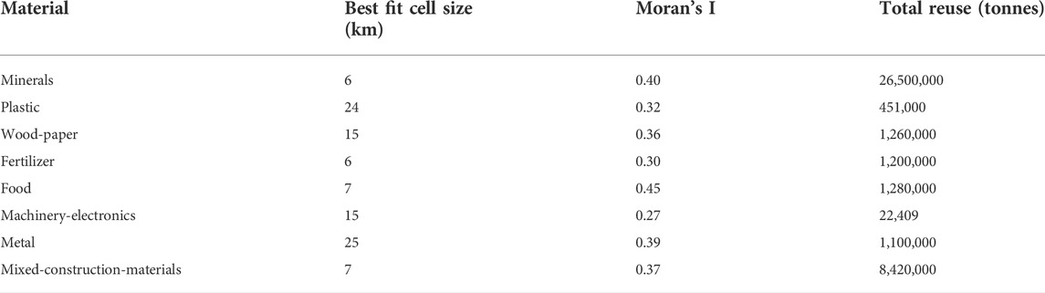
TABLE 1. Best fit cell size, Moran’s I, and total reuse in tonnes of each material.

Local Moran’s I—location of spatial clusters

Once the global Moran’s I and p-values have been determined for each material at each cell size, we are able to identify the locations of clusters for each material. There are four types of clusters: hot spots (red, high-high), cold spots (blue, low-low), doughnuts (light blue, low-high), and diamonds (pink, high-low). For more details on the four types, please refer to the materials and methods section. Figure 9 below shows, for each material, the locations of clusters using the minimum cell size, the “best fit” cell size derived from the previous global Moran’s I chart (Figure 8 and Table 1), and maximum cell size. The minimum and maximum cell size is determined by the smallest or largest cell size for each material that still produced a p-value lower than 0.05 for the global Moran’s I calculations (Figures 7, 8).

FIGURE 9

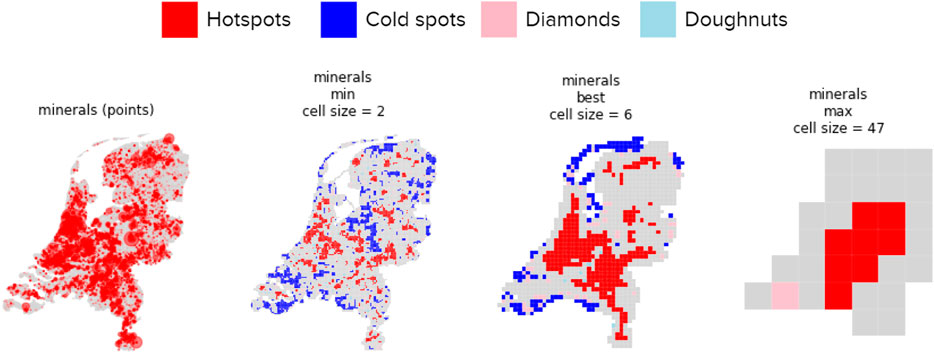
FIGURE 9. Maps of hotspots (red), cold spots (blue), doughnuts (light blue), and diamonds (pink) of mineral reuse in the Netherlands. For hotspot maps of all material types, please refer to the Supplementary Materials. Maps created by authors.

Discussion

The aim of this study was to understand the insights and caveats that can be derived from spatial clustering analysis of waste reuse locations. So far, this paper has presented the results of global and local Moran’s I analysis, on the strength, scale, and location of waste reuse clusters in the Netherlands. This section will elaborate on the insights and caveats that can be derived from these results.

Insights from results

The opportunities of using spatial clustering on waste reuse data to generate insights for circular regional development are presented in the paragraphs below.

In terms of global spatial autocorrelation results (global Moran’s I), if a material has a high global Moran’s I value and a p-value of less than 0.05, it indicates that its locations of reuse form a strong spatial pattern when displayed on a map. We can therefore conclude that the higher the Moran’s I for a material, the more affected it is by geography, and the more important it is to use a spatial perspective to analyze this material. All the materials considered, except for glass and textiles, had p-values lower than 0.05, meaning there could be spatial dependence, and that spatial clusters exist. This indicates that it would be fruitful to analyze these materials from a spatial perspective.

However, it is not meaningful to compare global Moran’s I values for different materials, because different materials have a “peak” Moran’s I at different cell sizes (for more explanation of cell sizes and Moran’s I, please refer to the results section). This can be shown in Figure 10 below, where mineral reuse locations have stronger clustering from cell sizes 2–12 km, while wood and paper reuse locations have stronger clustering from cell sizes 12–50 km. As seen in the graph, an answer cannot be given on whether minerals reuse locations are more spatially clustered than wood-paper, because this depends on the cell size used for the analysis.

FIGURE 10

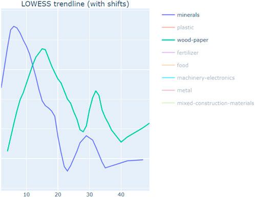
FIGURE 10. Comparing cell sizes for minerals and wood, chart created by authors.

The effect of cell size on the global Moran’s I value can be explained with Figure 11, where the map of mineral waste reuse is plotted as a 3D surface, with the x and y axis representing the longitude and latitude, and the z axis representing the amount (in kg) of mineral waste reuse.

FIGURE 11

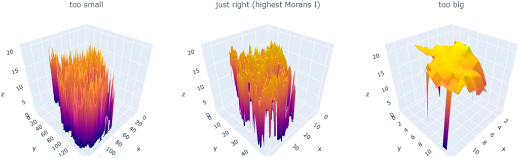
FIGURE 11. Using Moran’s I to optimize cell size, for the case of mineral reuse locations. For an interactive version, please see the Supplementary Materials document. Charts created by authors.

When the cell size is too small (∼2 km), the 3D plot is highly irregular; and when the cell size is too big (∼40 km), it resembles a flat surface. For both cases, the “resolution” of the grid is either too small or too big to form an identifiable spatial pattern. On the other hand, when plotting the cell size at which the global Moran’s I value is the highest (6 km), clear clusters can be identified in the form of identifiable peaks and troughs. This illustrates that the “best fit” cell size optimizes between cell sizes that are too small (or too detailed) and too big (or too vague).

Since the highest Moran’s I value for minerals occurs with 6 km·cell sizes, it can be stated that 6 km is the resolution at which mineral reuse locations should be spatially analyzed. Explained more technically, when the locations of mineral reuse is aggregated to a grid with cell sizes of 6 km, the strongest spatial pattern (clustering) can be observed. This also indicates that, within clusters of mineral waste reuse locations, most locations are, on average, 6 km away from each other.

As seen in Figure 12 below, locations of reuse for minerals, fertilizer, food, and mixed construction materials all have a global Moran’s I value that peaks at ∼7 km. On the other hand, the curves for plastic and metal both form an m-shape, with two peaks at different cell sizes. The first peak is similar for both materials, and happens at ∼20–25 km. The “best fit” cell size for wood-paper is somewhere in between the other materials, with an “best fit” cell size of ∼15 km. Finally, there was no clear “best fit” cell size for aggregating the reuse locations of machinery and electronics.

FIGURE 12

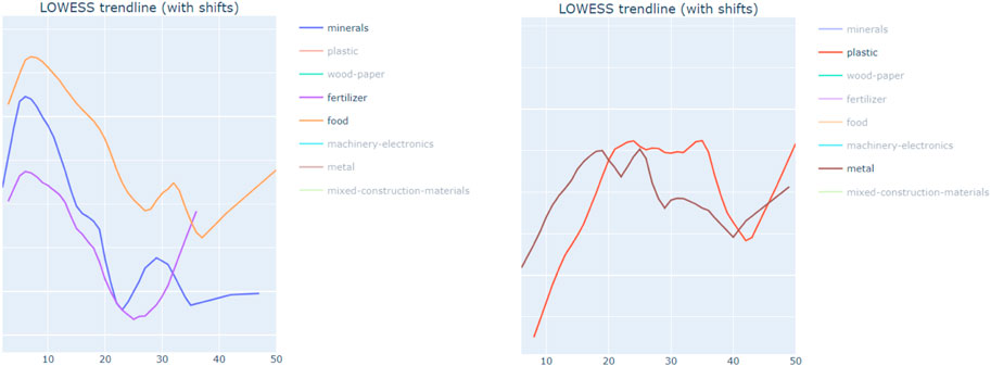
FIGURE 12. (A) Materials with best fit cell size of 7 km, chart created by authors. (B) Materials with best fit cell sizes higher than 15 km, chart created by authors.

Materials with a best fit cell size of 7 km (minerals, fertilizer, food, and mixed construction materials) are in the construction and agricultural industry; whereas materials with peaks of 20–25 km (plastic and metal) are more associated with consumer products. Arguably, the industries with smaller cell sizes (construction and agriculture) have more detailed spatial requirements than the industries with larger cell sizes (plastic and metal). Construction and agriculture are more closely related to cities—most of the activities of the construction industry happen in cities, whereas most agricultural activities happen away from cities.

Reuse of materials in the construction and agricultural industry could also be more distributed than other materials like metal or plastic. The reuse of metal would require large scale machinery at high costs, resulting in centralized locations; whereas reuse of minerals (such as concrete aggregate) can easily be done at any construction site in the country. For industries with distributed reuse locations, a reuse location could be found every few kilometers, which might explain the lower best fit cell sizes for the construction and agricultural industry.

From a policy or governance perspective, the resulting spatial scales for each material might indicate the governance level at which these materials could be manipulated—from neighborhoods, to municipalities, to provinces.

We also investigated how the “best fit” cell size of each material is affected by other attributes of the material: total kg reused for the whole country, percentage of areas with zero values, and the Moran’s I value. It was found that these attributes had a weak correlation with the “best fit” cell size, as seen in Figure 13 below. This indicates that the “best fit” cell size for each material provides insights that could not have been obtained using other material attributes, suggesting that there is value in finding the “best fit” cell size for each material.

FIGURE 13

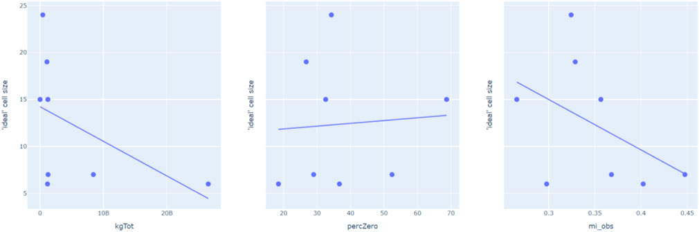
FIGURE 13. The effect of total kg (kgTot), percentage of zero values (percZero), Moran’s I (mi_obs) on best fit cell size (y-axis). Charts created by authors.

The potential insights gained from the local spatial correlation results are summarized in the paragraphs below. The results are shown as a map of hotspots, cold spots, doughnuts, and diamonds, and can be seen in Figure 8 in the results section.

For almost all materials, hotspots seem to be concentrated in the south of the country, roughly around the regions around Amsterdam, The Hague, Rotterdam, and Eindhoven. This is more extreme in the case of machinery and electronics, where the hotspots form a clear line running along the railway line from The Hague to Roermond. The exception is fertilizer reuse hotspots, which seem to be located around the north east of the country (Figure 14).

FIGURE 14

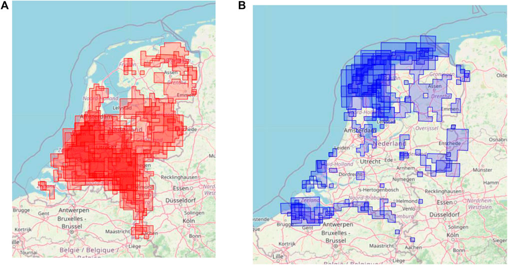
FIGURE 14. (A) Hotspots for all materials in the LMA dataset. Map created by authors. (B) Cold spots for all materials in the LMA dataset. Map created by authors.

Cold spots, on the other hand, indicate areas that have a significant cluster of low waste reuse. Most cold spots for most materials are located in the North-West of the Netherlands, where the Wadden islands are, as well as the South-West near the border with Belgium. The exception is food reuse locations, where cold spots are present on the north-east of the country as well (Figure 14).

Doughnuts indicate areas of low value surrounded by high value, whereas diamonds indicate areas of high value surrounded by low value. These location types are more distributed across the country, and don’t seem to form a distinguishable pattern.

The most evident insight from the local spatial autocorrelation maps, comes from the location of hotspots. These results can be used as a foundation for further research. Further investigation into hotspot locations using spatial regression methods can explain why hot spots are where they are. Additionally, hot spot maps can be used to imagine future (alternative) scenarios, understanding the co-location of future waste production, processing, and reuse.

Looking at the hot spot maps at different cell sizes, it becomes evident that the concept of “hot spot” should be applied to an area (or region), rather than a given point on the map. In the same way that a country can be financially wealthy at the national level but may have lower-income areas at the regional or local level, one location can be said to be a hot spot for one given cell size while the same point may or may not be part of a hot spot for other cell sizes. This suggests that one point on the map plays a different role within a neighborhood, city, province, or country. This has consequences for the realization of circular cities, as different spatial scales (neighborhood/municipal/regional/national) would result in different perspectives on the hot spots, prioritizing different areas as a consequence.

Research limitations

The limitations of using spatial clustering methods (Global and Local Moran’s I) on waste reuse data to generate insights for circular regional development are presented in the paragraphs below. For general limitations of using waste data to monitor the circular economy, please refer to the Supplementary Materials document.

Generally, spatial statistics require a large number of datapoints to be conducted. Therefore, for spatial statistical analysis, the phenomenon examined (in this paper, material reuse) needs to have many locations. Just because a material has many reuse locations, however, does not mean that it should be prioritized in a circular economy. As a consequence, spatial research on circular economy neglects materials which have a large environmental impact but are only concentrated in a few locations. In this study for example, glass and textiles were eliminated from the study, even though they may have a significant impact on the environment. Moreover, this study only focused on locations of waste reuse, without taking into account other activities in the waste-to-resources supply chain—locations of material stock, waste production, and waste processing.

Limitations for this study’s spatial analysis methods can be found in the interpretation of the “best fit” cell size and local Moran’s I. The “best fit” cell size should indicate the best resolution to examine a material by optimizing the trade-off between cell sizes that are too big and too small. This can be seen in the global Moran’s I results, where the “best fit” cell size for a material is the cell size at which spatial clustering is the strongest.

Following this logic, it would be expected that the hot spot maps made with the “best fit” cell size balances the trade-off between cell sizes that are too big or too small. When cell sizes are too small like Figure 15 below, the map is precise but inaccurate. When a hotspot is indicated on this map, the reader can indicate the precise 3 by 3 km squared location that is a hotspot, but at the same time, it’s more likely that this hotspot could have appeared by chance. In other words, this hotspot location might not have been statistically significant even if there had been minor changes to the material reuse rates there. On the other hand, when cell sizes are too big like Figure 15 below, the map is imprecise but accurate. When a hotspot is indicated on this map, the reader can only indicate a square of 49 × 49 km²—too large to be informative, and therefore imprecise. But, at the same time, it’s less likely that this hotspot could have appeared by chance.

FIGURE 15

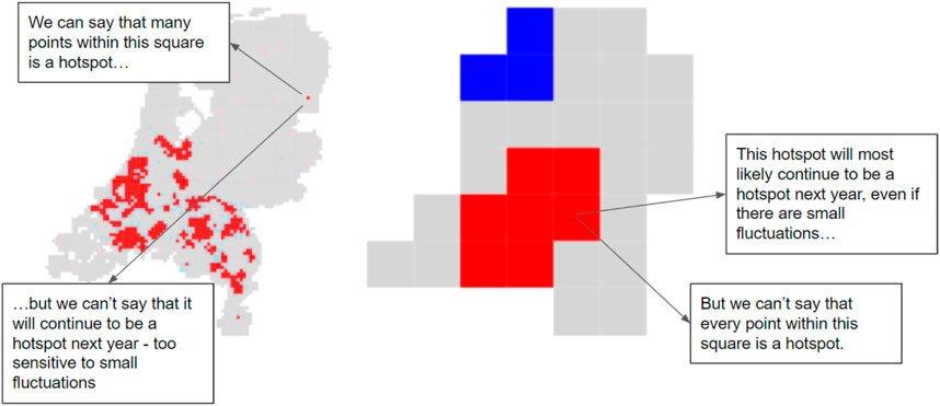
FIGURE 15. Trade off between large and small cell sizes for hot spot mapping. Maps and text boxes created by authors.

Although it is clear in theory that a hotspot map using the “best fit” cell size is the most informative, this is not so evident in practice. For example, when examining Figure 16 below, which shows the hotspot maps of food reuse locations with the minimum, “best fit,” and maximum cell size, it is tempting to say that the map with the minimum cell size is the most informative. While the minimum cell size map shows distinct areas as hotspots, the “best fit” cell size map shows hotspots as one large area covering almost the whole south side of the country.

FIGURE 16

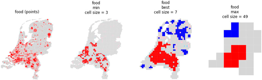
FIGURE 16. Comparing hot spot mapping with minimum, best fit, and maximum cell sizes. Maps created by authors.

This uncertainty from choosing between the minimum or best fit cell size indicates two potential conclusions: either that the best fit cell size is not relevant for other spatial analysis methods; or that the minimum cell size map gives a false impression of accuracy and the “best fit” cell size should be chosen. If we accept the second potential conclusion for the hotspot maps in Figure 14, the “best fit” cell size map (with cell size = 7 km) would provide the best possible representation of reality. Smaller cell sizes may look more precise and informative, but they are too sensitive to provide reliable information on the exact shape and number of clusters.

This indicates an important observation on spatial data analysis: while technological advancement has allowed for unprecedented precision on location data, spatial analysis results do not result in the same amount of precision. While LMA data has the precise street addresses for reuse locations, the hotspot maps created have a far lower precision, ranging from 6 to 25 km depending on the material.

Recommendations for further research

More experimentation can be done with spatial statistical methods to identify the spatial characteristics (such as land use, density, and accessibility) that affect the amount of waste reuse. In other words, this study has identified where waste reuse clusters are, the next step is to identify why the clusters are there. This can be done through spatial regression methods, which could indicate the relationship between waste reuse in a location with its associated spatial characteristics. An alternative would be to explore the same questions qualitatively, finding historical, social, or political reasons for waste reuse clusters. The factor of time could also be incorporated into the analysis, allowing a deeper understanding of how clusters change over the years. Additionally, waste material categorization can be improved to include information on re-usability. Material types can have a “re-usability score,” or could be categorized as a material, component, or product. An example can be found in (Sileryte et al., 2022).

Other spatial autocorrelation methods beyond Moran’s I, such as Geary’s C, can be used to analyze the same dataset of waste reuse. Comparing Moran’s I to other spatial autocorrelation methods would allow researchers to find out if the results of this study are merely an artifact of the Moran’s I statistic.

More understanding is needed for the entire “waste to resource supply chain.” Future studies could look beyond locations of waste reuse to examine locations of waste stock, production, and processing. A network perspective could be taken for this line of study, where aspects such centrality and travel distances could be incorporated.

More work could be done on linking spatial statistical results to policy ambitions. This would require a deeper understanding of the policy ambitions of the Netherlands and the European Union (EU), especially in terms of circular economy and spatial development (Van den Berghe and Verhagen 2021; Verhagen et al., 2021; Sileryte et al., 2022). have made a start here, developing tools that provide information to aid policy makers in making decisions related to circular regional development.

Finally, spatial statistical methods have the potential to simulate future scenarios to determine the feasibility of current policies related to circular regional development. Future demand for materials could be matched to future supply of secondary resources (Verhagen et al., 2021). Demand and supply matching could be simulated at different scales, to determine the feasibility of “closing the loop” at the neighborhood, city, provincial, or country level. Simulations can also be made from the perspective of disaster analysis, imagining future scenarios of extreme material scarcity, where limitations of the global supply chain could lead to substitutions with local secondary resources.

Conclusion

In conclusion, this paper added a spatial perspective to existing urban metabolism studies, by answering the research question, “How does analyzing the spatial clustering and hotspots of waste reuse locations generate insights for the circular economy, and what are the limitations of these insights?” The research question was answered by calculating the global and local spatial autocorrelation (global and local Moran’s I) for materials in the waste flow dataset of the national waste registry of the Netherlands.

The global Moran’s I values indicated that the reuse locations for all materials except for glass and textiles were spatially clustered in the Netherlands. The materials with spatial clustering are: minerals, mixed construction materials, wood and paper, metals, plastics, food, fertilizer, and machinery and electronics. By varying the cell sizes used to aggregate the reuse location data, it was found that each material had an “best fit” cell size that optimized the trade-offs between cell sizes too large and too small. Materials associated with the construction and agriculture industry (minerals, mixed construction materials, food, and fertilizer) had an “best fit” cell size of 7 km, wood and paper of 15 km, metals and plastics of ∼20–25 km, but machinery and electronics had no clear “best fit” cell size. Local spatial autocorrelation results were used to generate maps of hotspots, cold spots, doughnuts, and diamonds for each material.

From the results, the potential and limitations of using these results to find insights for circular regional development were identified. In terms of potential insights, the “best fit” cell size identified for each material could indicate the scale or resolution at which the material could best be understood with additional spatial analysis, the potential governance level of that material (neighborhoods, cities, provinces, and country), or its spatial attributes, such as its relationship to urban areas or level of centralization. The “best fit” cell size is the cell size that maximizes Moran’s I and allows the researcher to display the (aggregated) map that is the most highly clustered. The hotspots maps generated from local Moran’s I values indicate which regions could facilitate reuse activities for a particular material.

On the other hand, there are also limitations to using spatial analysis results for circular economy insights. Waste data limits the focus of studies to material reuse strategies (such as recycling or incineration), while ignoring product life extension strategies (such as design or repair). Waste data is also difficult to categorize—categories that are too general, such as “metal” for example, do not provide sufficient information about the type of metal. Categorizations in waste dataset also often cannot match the specificity of new product material requirements. Results also lack the network or relational perspective of the whole “waste to resource supply chain.” More generally, spatial analysis for a circular economy may fall into the trap of over-emphasizing on materials associated with many locations, rather than a high environmental impact.

This study makes both theoretical and practical contributions to existing knowledge on urban metabolism and circular economy. In terms of theoretical contributions, we have shown an example of using spatial analysis methods to study waste reuse locations, in order to add a spatial perspective to the existing literature on regional material flows (urban metabolism) and urban governance (circular cities) for a circular economy.

The spatial perspective allows for a more detailed understanding of the locations of waste-to-resource flows by examining smaller spatial units—looking at waste reuse per neighborhood rather than per city, province, or country. Moreover, this perspective provides more objective descriptions of a material’s spatial characteristics (such as spatial clustering, scale), which goes beyond geo-visualization in the form of mapping. By varying aggregation resolutions to find an “best fit” cell size, this study also contributes a potential method for addressing the modifiable areal unit problem (MAUP).

Finally, with further development, we hope that this line of research could ultimately inform spatial policy, allowing existing circular city plans of municipalities, provinces, and countries to expand their reach beyond governance and policy and towards spatial and regional planning.

Data availability statement

The data supporting the conclusions of this article will be made available by the authors in aggregated form of grid size 5 km. The raw data cannot be shared as it contains confidential data of private companies.

Author contributions

Funding acquisition: DP. Investigation, methodology, and project administration: TT. Guidance on statistical analysis: AD. Writing: TT. Supervision, review and editing: AD, DP, AvT, and AW.

Funding

This research received funding from the European Union’s Horizon 2020 Research and Innovation Programme under grant agreement No. 821479.

Conflict of interest

The authors declare that the research was conducted in the absence of any commercial or financial relationships that could be construed as a potential conflict of interest.

Publisher’s note

All claims expressed in this article are solely those of the authors and do not necessarily represent those of their affiliated organizations, or those of the publisher, the editors and the reviewers. Any product that may be evaluated in this article, or claim that may be made by its manufacturer, is not guaranteed or endorsed by the publisher.

Supplementary material

The Supplementary Material for this article can be found online at: https://www.frontiersin.org/articles/10.3389/fbuil.2022.954642/full#supplementary-material

References

Amenta, L., Attademo, A., Remøy, H., Berruti, G., Cerreta, M., Formato, E., et al. (2019). Managing the transition towards circular metabolism: Living labs as a Co-creation approach. Up 4 (3), 5–18. doi:10.17645/up.v4i3.2170

CrossRef Full Text | Google Scholar

Anselin, L. (1995). Local indicators of spatial association-LISA. Geogr. Anal. 27 (2), 93–115. doi:10.1111/j.1538-4632.1995.tb00338.x

CrossRef Full Text | Google Scholar

Anselin, L. (2020). Moran scatter plot. Mitacs Project Report. Available at: https://geodacenter.github.io/workbook/5a_global_auto/lab5a.html#moran-scatter-plot.

Google Scholar

Antczak, E. (2020). Regional patterns in dumping sites in Poland - analysis in context of the new "sustainable" waste policy. Pol. J. Environ. Stud. 29 (2), 1037–1049. doi:10.15244/pjoes/108484

CrossRef Full Text | Google Scholar

Arciniegas, G., Šileryté, R., Dąbrowski, M., Wandl, W., Dukai, B., Bohnet, M., et al. (2019). A geodesign decision support environment for integrating management of resource flows in spatial planning. Up 4 (3), 32–51. doi:10.17645/up.v4i3.2173

CrossRef Full Text | Google Scholar

Bakker, C. A., Hollander, M. C. D., Hinte, E. V., and Zijlstra, Y. (2019). Products that last - product design for circular business models. TU Delft Library/Marcel den Hollander IDRC.

Google Scholar

Baptista, R., and Swann, G. M. (1999). A comparison of clustering dynamics in the US and UK computer industries. J. Evol. Econ. 9 (3), 373–399. doi:10.1007/s001910050088

CrossRef Full Text | Google Scholar

Bocken, N. M. P., de Pauw, I., Bakker, C., and van der Grinten, B. (2016). Product design and business model strategies for a circular economy. J. Industrial Prod. Eng. 33 (5), 308–320. doi:10.1080/21681015.2016.1172124

CrossRef Full Text | Google Scholar

Bolger, K., and Doyon, A. (2019). Circular cities: Exploring local government strategies to facilitate a circular economy. Eur. Plan. Stud. 27 (11), 2184–2205. doi:10.1080/09654313.2019.1642854

CrossRef Full Text | Google Scholar

Broto, V. C., Allen, A., and Rapoport, E. (2012). Interdisciplinary perspectives on urban metabolism. J. Industrial Ecol. 16 (6), 851–861. doi:10.1111/j.1530-9290.2012.00556.x

CrossRef Full Text | Google Scholar

Brunner, P. H. (2007). Reshaping urban metabolism. J. Ind. Ecol. 11 (2), 11–13. doi:10.1162/jie.2007.1293

CrossRef Full Text | Google Scholar

Cheniti, H., Cheniti, C., and Brahamia, K. (2021). Use of GIS and Moran's I to support residential solid waste recycling in the city of Annaba, Algeria. Environ. Sci. Pollut. Res. 28 (26), 34027–34041. doi:10.1007/s11356-020-10911-z

CrossRef Full Text | Google Scholar

Codoban, N., and Kennedy, C. A. (2008). Metabolism of neighborhoods. J. Urban Plann. Dev. 134 (1), 21–31. doi:10.1061/(asce)0733-9488(2008)134:1(21)

CrossRef Full Text | Google Scholar

den Hollander, M. C. D., Bakker, C. A., and Hultink, E. (2017). Product design in a circular economy: Development of a typology of key concepts and terms. J. Industrial Ecol. 21 (3), 517–525. doi:10.1111/jiec.12610

CrossRef Full Text | Google Scholar

Dijst, M., Worrell, E., Böcker, L., Brunner, P., Davoudi, S., Geertman, S., et al. (2018). Exploring urban metabolism-Towards an interdisciplinary perspective. Resour. Conservation Recycl. 132, 190–203. doi:10.1016/j.resconrec.2017.09.014

CrossRef Full Text | Google Scholar

European Commission (2020). A new circular economy action plan. Brussels, Belgium: The EU’s new circular action plan paves the way for a cleaner and more competitive Europe.

Google Scholar

Furlan, C., Wandl, A., Cavalieri, C., and Unceta, P. M. (2022). “Territorialising circularity,” in Regenerative territories: Dimensions of circularity for healthy metabolisms. Editors L. Amenta, M. Russo, and A. van Timmeren (Springer), Vol. 128, 31–49. doi:10.1007/978-3-030-78536-9_2

CrossRef Full Text | Google Scholar

Geissdoerfer, M., Savaget, P., Bocken, M., Hultink, P., and Jan Hultink, E. (2017). The Circular Economy - a new sustainability paradigm? J. Clean. Prod. 143, 757–768. doi:10.1016/j.jclepro.2016.12.048

CrossRef Full Text | Google Scholar

Geng, Y., Zhang, L., Chen, X., Xue, B., Fujita, T., and Dong, H. (2014). Urban ecological footprint analysis: A comparative study between shenyang in China and kawasaki in Japan. J. Clean. Prod. 75, 130–142. doi:10.1016/j.jclepro.2014.03.082

CrossRef Full Text | Google Scholar

Getis, A., and Ord, J. K. (1992). The analysis of spatial association by use of distance statistics. Geogr. Anal. 24 (3), 189–206. doi:10.1111/j.1538-4632.1992.tb00261.x

CrossRef Full Text | Google Scholar

GIS Geography (2022). Maup - scale effect GIS geography. Avaliable At: https://gisgeography.com/maup-modifiable-areal-unit-problem/.

Google Scholar

GIS Lounge (2018). MAUP zone effect. AvaliableAt: https://www.gislounge.com/modifiable-areal-unit-problem-gis/.

Google Scholar

Graedel, T., Reck, B., Ciacci, L., and Passarini, F. (2019). On the spatial dimension of the circular economy. Resources 8 (1), 32. doi:10.3390/resources8010032

CrossRef Full Text | Google Scholar

Hanemaaijer, A., Kishna, M., Brink, H., Koch, J., Gerdien Prins, A., and Rood, T. (2021). Netherlands integral circular economy report 2021. Report.

Google Scholar

Hassan, M. M., Alenezi, M. S., and Good, R. Z. (2020). Spatial pattern analysis of manufacturing industries in keraniganj, dhaka, Bangladesh. GeoJournal 85 (1), 269–283. doi:10.1007/s10708-018-9961-5

CrossRef Full Text | Google Scholar

Huo, X-N., Li, L., Sun, D. F., Zhou, L. D., and Li, B. G. (2012). Combining geostatistics with Moran's I analysis for mapping soil heavy metals in beijing, China. Ijerph 9 (3), 995–1017. doi:10.3390/ijerph9030995

PubMed Abstract | CrossRef Full Text | Google Scholar

Kalmykova, Y., Sadagopan, M., and Rosado, L. (2018). Circular economy - from review of theories and practices to development of implementation tools. Resour. Conservation Recycl. 135, 190–201. doi:10.1016/j.resconrec.2017.10.034

CrossRef Full Text | Google Scholar

Keirstead, J., and Sivakumar, A. (2012). Using activity-based modeling to simulate urban resource demands at high spatial and temporal resolutions. J. Industrial Ecol. 16 (6), 889–900. doi:10.1111/j.1530-9290.2012.00486.x

CrossRef Full Text | Google Scholar

Kennedy, J. C., Cuddihy, J., and Engel-Yan, J. (2007). The changing metabolism of cities. J. Ind. Ecol. 11 (2), 43–59. doi:10.1162/jie.2007.1107

CrossRef Full Text | Google Scholar

Kennedy, P., Pincetl, S., and Bunje, P. (2011). The study of urban metabolism and its applications to urban planning and design. Environ. Pollut. 159 (8–9), 1965–1973. doi:10.1016/j.envpol.2010.10.022

PubMed Abstract | CrossRef Full Text | Google Scholar

Kirchherr, J., Reike, D., and Hekkert, M. (2017). Conceptualizing the circular economy: An analysis of 114 definitions. Resour. Conservation Recycl. 127, 221–232. doi:10.1016/j.resconrec.2017.09.005

CrossRef Full Text | Google Scholar

Kirkegaard, O. W. E. (2015). Moran’s I scheme.” some methods for measuring and correcting for spatial autocorrelation. AvaliableAt: https://thewinnower.com/papers/2847-some-methods-for-measuring-and-correcting-for-spatial-autocorrelation.

Google Scholar

Li, H., and Kwan, M. P. (2018). Advancing analytical methods for urban metabolism studies. Resour. Conservation Recycl. 132, 239–245. doi:10.1016/j.resconrec.2017.07.005

CrossRef Full Text | Google Scholar

López, F. A., and Páez, P. (2017). Spatial clustering of high-tech manufacturing and knowledge-intensive service firms in the Greater Toronto Area. Can. Geogr./Le Géogr. Can. 61 (2), 240–252. doi:10.1111/cag.12326

CrossRef Full Text | Google Scholar

Malmberg, A., and Maskell, P. (2002). The elusive concept of localization economies: Towards a knowledge-based theory of spatial clustering. Environ. Plan. A 34 (3), 429–449. doi:10.1068/a3457

CrossRef Full Text | Google Scholar

Marin, J., Alaerts, L., and Van Acker, K. (2020). A materials bank for circular leuven: How to monitor 'messy' circular city transition projects. Sustainability 12 (24), 10351. doi:10.3390/su122410351

CrossRef Full Text | Google Scholar

Moore, J., Kissinger, M., and Rees, W. E. (2013). An urban metabolism and ecological footprint assessment of metro vancouver. J. Environ. Manag. 124, 51–61. doi:10.1016/j.jenvman.2013.03.009

CrossRef Full Text | Google Scholar

Openshaw, S. (1983). “The modifiable areal unit problem,” in Concepts and techniques in modern geography (Norfolk: Geo Books).

Google Scholar

Prendeville, S., Cherim, E., and Bocken, N. (2018). Circular cities: Mapping six cities in transition. Environ. Innovation Soc. Transitions 26, 171–194. doi:10.1016/j.eist.2017.03.002

CrossRef Full Text | Google Scholar

Rawlins, B. G., Lark, R. M., O'Donnell, K. E., Tye, A. M., and Lister, T. R. (2005). The assessment of point and diffuse metal pollution of soils from an urban geochemical survey of sheffield, england. soil use manage 21 (4), 353–362. doi:10.1079/SUM2005335

CrossRef Full Text | Google Scholar

Sileryte, R., Sabbe, A., Bouzas, V., Meister, K., Wandl, W., and van Timmeren, A. (2022). European waste statistics data for a circular economy monitor: Opportunities and limitations from the Amsterdam metropolitan region. J. Clean. Prod. 358, 131767. doi:10.1016/j.jclepro.2022.131767

CrossRef Full Text | Google Scholar

Song, Y., Gil, J., Wandl, W., and Timmeren, A. (2018). Evaluating sustainable urban development using urban metabolism indicators in urban design. Eur. XXI 34, 5–22. doi:10.7163/Eu21.2018.34.1

CrossRef Full Text | Google Scholar

Sprecher, B., Verhagen, T., Sauer, M., Baars, M., Heintz, J., and Fishman, T. (2021). Material intensity database for the Dutch building stock: Towards big data in material stock analysis. J Industrial Ecol. 26, 272–280. doi:10.1111/jiec.13143

CrossRef Full Text | Google Scholar

Statistics Netherlands (2020). How much do we recycle? The Netherlands in numbers. AvaliableAt: https://longreads.cbs.nl/the-netherlands-in-numbers-2020/how-much-do-we-recycle/.

Google Scholar

Stephan, A., and Athanassiadis, A. (2017). Quantifying and mapping embodied environmental requirements of urban building stocks. Build. Environ. 114, 187–202. doi:10.1016/j.buildenv.2016.11.043

CrossRef Full Text | Google Scholar

Sunny, S. A., and Shu, S. (2019). Investments, incentives, and innovation: Geographical clustering dynamics as drivers of sustainable entrepreneurship. Small Bus. Econ. 52 (4), 905–927. doi:10.1007/s11187-017-9941-z

CrossRef Full Text | Google Scholar

Tanikawa, H., Fishman, T., Okuoka, K., and Sugimoto, K. (2015). The weight of society over time and space: A comprehensive account of the construction material stock of Japan, 1945-2010. J. Industrial Ecol. 19 (5), 778–791. doi:10.1111/jiec.12284

CrossRef Full Text | Google Scholar

Tjallingii, S. (1996). Ecological conditions. Strategies and structures in environmental planning. Delft: Institutional Repository. Thesis.

Google Scholar

Van den Berghe, K., and Verhagen, T. (2021). Making it concrete: Analysing the role of concrete plants' locations for circular city policy goals. Front. Built Environ. 7, 748842. doi:10.3389/fbuil.2021.748842

CrossRef Full Text | Google Scholar

Van den Berghe, K., and Vos, M. (2019). Circular area design or circular area functioning? A discourse-institutional analysis of circular area developments in Amsterdam and utrecht, The Netherlands. Sustainability 11 (18), 4875. doi:10.3390/su11184875

CrossRef Full Text | Google Scholar

Verhagen, T. J., Sauer, M., van der Voet, E., and Sprecher, B. (2021). Matching demolition and construction material flows, an urban mining case study. Sustainability 13 (2), 653. doi:10.3390/su13020653

CrossRef Full Text | Google Scholar

Wandl, A. (2020). Territories-in-between: A cross-case comparison of dispersed urban development in Europe. Delft: A+BE | Architecture and the Built Environment, Vol. 2.

Google Scholar

Williams, J. (2019b). Circular cities. Urban Stud. 56 (13), 2746–2762. doi:10.1177/0042098018806133

CrossRef Full Text | Google Scholar

Williams, J. (2019a). Circular cities: Challenges to implementing looping actions. Sustainability 11 (2), 423. doi:10.3390/su11020423

CrossRef Full Text | Google Scholar

Wolman, A. (1965). The metabolism of cities. Sci. Am. 213 (3), 178–190. doi:10.1038/scientificamerican0965-178

CrossRef Full Text | Google Scholar

Zhang, L., Zhong, Y., and Geng, Y. (2019). A bibliometric and visual study on urban mining. J. Clean. Prod. 239, 118067. doi:10.1016/j.jclepro.2019.118067

CrossRef Full Text | Google Scholar

Zhang, Y. (2013). Urban metabolism: A review of research methodologies. Environ. Pollut. 178, 463–473. doi:10.1016/j.envpol.2013.03.052

PubMed Abstract | CrossRef Full Text | Google Scholar

Zhao, K., Fu, W., Liu, X., Huang, D., Zhang, C., Ye, Z., et al. (2014). Spatial variations of concentrations of copper and its speciation in the soil-rice system in wenling of southeastern China. Environ. Sci. Pollut. Res. 21 (11), 7165–7176. doi:10.1007/s11356-014-2638-9

CrossRef Full Text | Google Scholar

Zhu, X. (2014). GIS and urban mining. Resources 3 (1), 235–247. doi:10.3390/resources3010235

CrossRef Full Text | Google Scholar