 Joshua C. Agar1,2*
 Julius Rhoan T. Lustro3,2
 Percival Magpantay4,2John Richard E. Hizon4,2Joseph Gerard T. Reyes3,2
- 1Institute of Civil Engineering, College of Engineering, University of the Philippines Diliman, Quezon City, Philippines
- 2UP Center for Air Research in Urban Environments Research Program, University of the Philippines Diliman, Quezon City, Philippines
- 3Department of Mechanical Engineering, College of Engineering, University of the Philippines Diliman, Quezon City, Philippines
- 4Electrical and Electronics Engineering Institute, College of Engineering, University of the Philippines Diliman, Quezon City, Philippines
With the COVID-19 pandemic still ongoing, there is a need to ensure that people are not subjected to the risk of getting infected with the disease. Since COVID-19 is airborne, engineering controls must be provided to monitor and mitigate the spread of the disease in the air. One of the measures is to ensure proper ventilation within indoor spaces where superspreader events were previously documented in poorly ventilated spaces. CO2 levels reflect the rate at which the used air within is replaced and, therefore, can be used as a proxy for COVID-19 risk. This study developed economical CO2 monitors which are deployed across indoor spaces and public transportation, such as air-conditioned jeepneys, to communicate the risk. Using the least squares method on the first-order ODE of mass balance, a multivariate method is devised for deriving the occupancy and the ventilation rate from the recorded CO2 levels. Using the multivariate method, the ventilation rates of different indoor spaces are determined and used for the subsequent computations using the Wells–Riley model to derive the respective infection risk, particularly of COVID-19.
1 Introduction
At the onset of the ongoing COVID-19 pandemic, indoor spaces are identified to have higher infection rates than outdoor spaces (Qian, et al., 2021). Poor ventilation has been attributed to many of the superspreader events (Miller, et al., 2021). Because of the low air changes due to poor ventilation, SARS-CoV-2, the virus that causes COVID-19, is found to be deposited on ventilation ducts and other surfaces with greater distances which cannot be explained by droplet transmissions (Nissen, et al., 2020). A literature review on droplet transmission shows no direct evidence for ballistic droplets as the route of transmission of any diseases (Chen, et al., 2020). Inhalation of the suspended pathogenic aerosols is determined to have been causing COVID-19 infections (Greenhalgh, et al., 2021) as confirmation that SARS-CoV-2 is detected within particulate matter captured in the air (López, et al., 2021). As a result, medical insights on respiratory virus transmission and the subsequent infection control programs have been undergoing a paradigm shift in acknowledging airborne transmissions (Klopmas, et al., 2021) despite historical resistance (Jimenez, et al., 2022).
Initially for measles, which was then identified as an airborne disease (Wells, 1955), an epidemiological model was developed to estimate its infection risk in classrooms (Riley, et al., 1978). The application of the model has been extended to tuberculosis (Gammaitoni and Nucci, 1997) and then to COVID-19 (Buonnano, et al., 2020). This enables readily quantifying the practical infection risk by compiling all the previous superspreader events due to shared room air transmission (Peng, et al., 2022) and using CO2 as the relative risk indicator (Bazant, et al., 2021; Peng and Jimenez, 2021).
However, the formulation of using CO2 as a relative risk indicator mainly assumes that the recorded CO2 level has been the steady-state level. When not in steady-state conditions, the ventilation rate must be derived from the prior knowledge of the occupancy. Such a condition is true for buildings with a low supply of outdoor air, provided that the rate does not vary in time (Rudnick and Milton, 2003). This study aims to develop a multivariate technique for deriving occupancy and ventilation rates simultaneously. In addition, this study also aims to create a low-cost CO2 monitor which will cover the physical measurement of the CO2 concentration. These will enable the study to determine the infection risk of COVID-19, the disease that is being closely monitored due to the ongoing pandemic, over indoor spaces such as classrooms and the common modes of transportation present in the Philippines.
2 Materials and methods
2.1 Multivariate technique on deriving occupancy and ventilation
This study assumes a well-mixed indoor room where the CO2 emissions from the occupants are evenly distributed across the room while air is constantly replaced by outdoor air with a uniform outdoor CO2 concentration. This results in a first-order ordinary differential equation:
where
This study will focus on the differential equation given in Eq. 1. The first-order ODE is discretized and restated as
where
The emission rate
The whole Eq. 2 is multiplied with
This study assumes that CO2 readings from the CO2 sensors are measured at regular intervals, although it can also work for readings at irregular intervals. As this study maintained that only integers will be used to simplify computations for the target ESP32 microcontroller,
Eq. 3 will then have two unknowns, namely, the estimated occupancy
With a known volume
To determine the stability of the solution, the analytical solution of the first-order ODE is derived:
Substituting the analytical solution to the discrete first-order ODE and simplifying will result in the relationship between the time step and ventilation rate in a stable solution:
Given that the sensor transmits integer values for the CO2 levels, for the solution to remain stable, the following relation must be satisfied as values less than zero reflect that the computed ventilation rates are negative, while values greater than 1.5 reflect that the time scale for the temporal averaging is reducing the resolution of the solution. Figure 1 shows a sample time history of ventilation rate estimates over different given time steps.
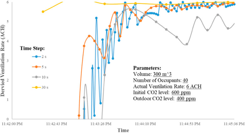
FIGURE 1. Solution stability on a sample case.
Alternatively, if the number of occupants
2.2 Wells–Riley model
Using the derived ventilation rates and occupancy, the infection risk due to airborne diseases can be computed using the Wells–Riley model.
where
where
Scenario the worst case, which is the exposure to the steady-state condition, by substituting the analytical solution for the mixing equation of quanta in Eq. 11 and substituting the Wells–Riley Model in Eq. 10 yield Eq. 12 for the infection risk as a function of time, volume, ventilation rate, room volume, and the reduction factors of the respiratory protection:
Three infection risk cases are then explored for each variant in each setting: 1) with the occupants not wearing masks, 2) two-way masking with surgical masks, and 3) two-way masking with N95 masks.
2.3 CO2 monitoring
This study deployed these CO2 monitors, shown in Figure 2, in classrooms of the UP Institute of Civil Engineering. This study has also tackled making a reliable yet economical CO2 monitor for potential mass distribution. Winsen MH-Z19E NDIR sensors are used, which are connected to an ESP32 module which then transmits the CO2 readings through the internet of things (IoT) using its built-in Bluetooth and WiFi module. The readings and the estimates on ventilation rates will be displayed through a connected LCD module.
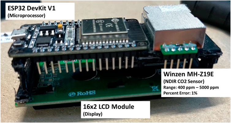
FIGURE 2. Components of the CO2 monitor device.
This study deployed these CO2 monitors in classrooms of the UP Institute of Civil Engineering. Four scenarios were tested: when people are occupying the room while the room is enclosed for air-conditioning (stale air seeps out through leaks), when the room is occupied by the one conducting the measurement, when there is one-way ventilation, and when there is two-way ventilation. This study has also deployed these CO2 monitors in public transportation during operation. The list and the details of the public transportation are shown in Figure 3.
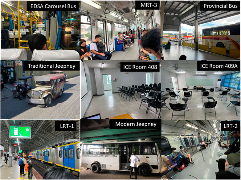
FIGURE 3. Indoor spaces and public transportation subject in CO2 monitoring.
3 Results and discussion
3.1 Classroom
The CO2 levels in the first classroom (Volume: 154 m3) were monitored during class, as shown in Figure 4. The algorithm has estimated a lower occupancy rate of eight people while estimating a ventilation rate of 0.1 ACH. This is because of the lower breathing activity rate in the classroom due to the students listening only to the lecture, resulting in lower CO2 levels. Artificially, plugging the actual number of occupants of 20 using Eq. 9 gives a ventilation rate of 3.2 ACH, which does not fit the ventilation rates of a typical fully enclosed room.
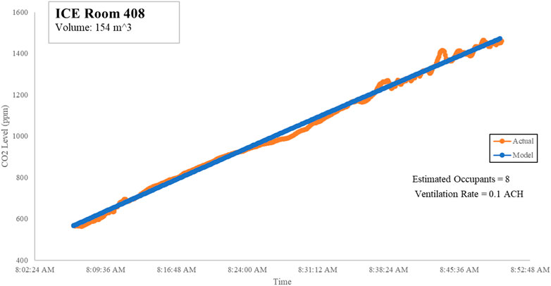
FIGURE 4. ICE Room 408 CO2 readings.
On the other hand, the measurements in Room 409A were conducted right after the students had vacated the room at CO2 levels of 1797 ppm. Eqs 4, 5 struggled to determine occupancy and ventilation rates on downward trends as the equations gave negative values, so Eq. 9 was used instead, as shown in Figure 5.
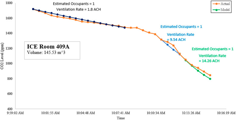
FIGURE 5. ICE Room 409A CO2 readings when air only exits through the leaks (dark blue), when windows are opened (light blue), and when two-way ventilation is implemented (green).
Room 409A has an adjacent room that was separated by a removable barrier which can introduce more leaks for the stale air within to pass through. As a result, a ventilation rate of 1.8 ACH was determined. However, opening the windows on just one side of the room results in the ventilation rate increasing to 9.54 ACH. Moreover, opening the door on the other side of the room to facilitate two-way ventilation results in the ventilation rate increasing further to 14.26 ACH.
3.2 Traditional jeepney
CO2 levels were also measured in a traditional jeepney. Traditional jeepneys are windowless public transport vehicles, with both sides open. Their typical seating capacity ranges from 12 to 18 for short type and up to 26–32 for long type. A short-type jeepney was considered in this study.
The jeepney initially was stationary as it waited for passengers to fully board. As shown in Figure 6A, the ventilation rate was determined to be 47.56 ACH. As the jeepney started to move, the ventilation rate further increased to 151.54 ACH, as shown in Figure 6B.
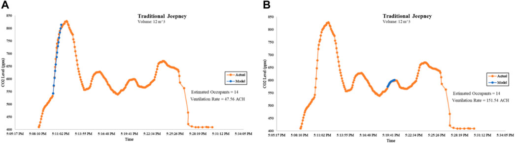
FIGURE 6. CO2 levels at a traditional jeepney. (A) Derivation of the ventilation rate when the jeepney was stationary and (B) derivation of the ventilation rate when the jeepney was in motion.
The algorithm programmed to the microcontroller units resets its multivariate analysis once it detects an inflection point as this indicates a change in the occupancy and/or the ventilation rate. For example, at the time frame shown in Figure 6A, the jeepney was stationary. After that, the jeepney began moving, resulting in a change in ventilation rates.
3.3 Modern jeepney
Air-conditioned minibuses, also known as the “Modern Jeepneys,” were also subjected to CO2 measurements. Unlike air-conditioned commuter vehicles such as buses or trains, these modern jeepneys follow the operation of traditional jeepneys, i.e., they stop and open the doors randomly whenever a passenger gets on or off. This scenario creates imperfect mixing. Their typical seating capacity is 23, with up to five people standing on the aisle.
As shown in Figure 7, due to the imperfect mixing within the modern jeepneys, Eqs 4, 5 estimated high emission rates and high ventilation rates. So, Eq. 9 was instead used, using the known occupant count of 26 people, resulting in a ventilation rate of 1.23 ACH.
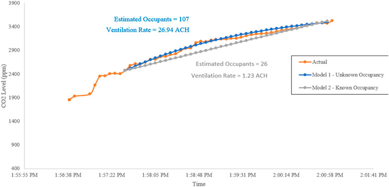
FIGURE 7. CO2 levels at the modern jeepney.
3.4 MRT-3
To capture a perfectly mixed environment for the derivation of the ventilation rates, the CO2 measurements on the MRT 3000 trains of the MRT-3 lines are focused on the first leg of the trip before the doors reopened on the next station, as shown in Figure 8. MRT 3000 coaches are air-conditioned, and the windows on both sides are closed. The derived ventilation rate was 2.78 ACH.
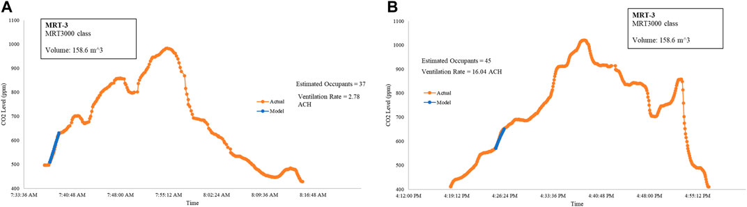
FIGURE 8. Derivation of the ventilation rate on MRT-3 trains at the first leg of the northbound trip (A) and mid-journey of the southbound trip (B).
Once the doors are opened, as shown in Figure 8B, the ventilation rate increases to 16.04 ACH. Both the ACH reports are done, given that the estimated number of occupants matched the actual number of occupants.
The train direction and the time presented in Figure 8 are at a moderately busy window of MRT-3 operations. Note that a sudden influx of passengers due to rush hour can plummet the ventilation rate. One way to increase the ventilation rate in commuter trains is by opening the windows (Shinohara, et al., 2021).
3.5 LRT-2
Unlike MRT-3, the trains on LRT-2 have a continuous air-conditioned train cabin extending from the front to the back. The windows on both sides are also closed. As the train accelerates, the air from the front rushes to the back of the train, resulting in internal compartmentalization of the inside air. As shown in Figure 9, despite Eqs 4, 5 having good estimates of the occupancy, the ventilation rate was estimated to be at 15.34 ACH.
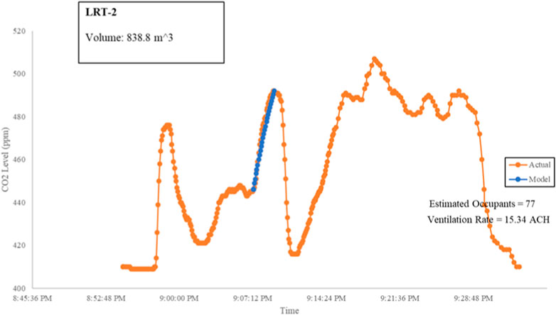
FIGURE 9. Estimation of ventilation rates from CO2 levels within LRT-2 trains.
3.6 LRT-1
This study has also covered the modern air-conditioned trains of the LRT-1 line. Within LRT-1, the train was divided into three separate train wagons. The windows on both sides were also closed. The passenger count within the train wagon was constant from the EDSA Station to Central Station. The CO2 levels within that interval were used in Eqs 4, 5, as shown in Figure 10.
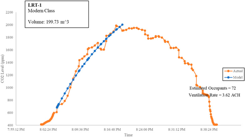
FIGURE 10. Estimation of the ventilation rates from CO2 levels within LRT-1 trains.
Although doors were opening and closing during the train stops at train stations, the drop in CO2 levels and the change in ventilation rates were not observed as the passengers were not moving within and passengers stood by the doors. Northbound LRT-1 trains are typically busy at this time of the evening as they ferry people who are working in Pasay city, Makati city, and Manila city to North Manila. The average ventilation rate measured from the EDSA Station to Central Station was determined to be at 3.62 ACH. Eqs 4, 5 returned the negative values for occupancy and ventilation rate when tested over the downward trend.
3.7 EDSA Carousel bus
The CO2 measurements were done during the rush hour when the air-conditioned buses were queuing at the bus stops. The windows on both sides are closed. Figure 11A shows Eqs 4, 5 being tested at the time the bus was moving at a slow pace, while Figure 11B shows Eqs 4, 5 being tested at the time the bus was stationary as it queued for the bus stop.
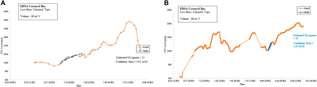
FIGURE 11. Estimation of ventilation rates from CO2 levels within EDSA Carousel buses. (A) Northbound and (B) southbound.
Upon Eqs 4, 5 computing the same occupancy as the actual occupancy, the ventilation rates were determined. The ventilation rate of the EDSA Carousel bus when stationary was 2.29 ACH, while when in motion, the ventilation rate was 4.92 ACH.
3.8 Provincial bus
CO2 levels were measured in the first continuous leg of the 12-h journey onboard an air-conditioned provincial bus without the doors opening. As shown in Figure 12, upon Eqs 4, 5 computing the same number of people as with the actual number of people, the ventilation rate was determined to be equal to 2.49 ACH.

FIGURE 12. Estimation of the ventilation rates from CO2 levels within a provincial bus.
3.9 COVID-19 infection risk
With the ventilation rates derived, the infection risks are determined in Tables 1, 2, and 3 for the Alpha, Delta, and Omicron variants, respectively.
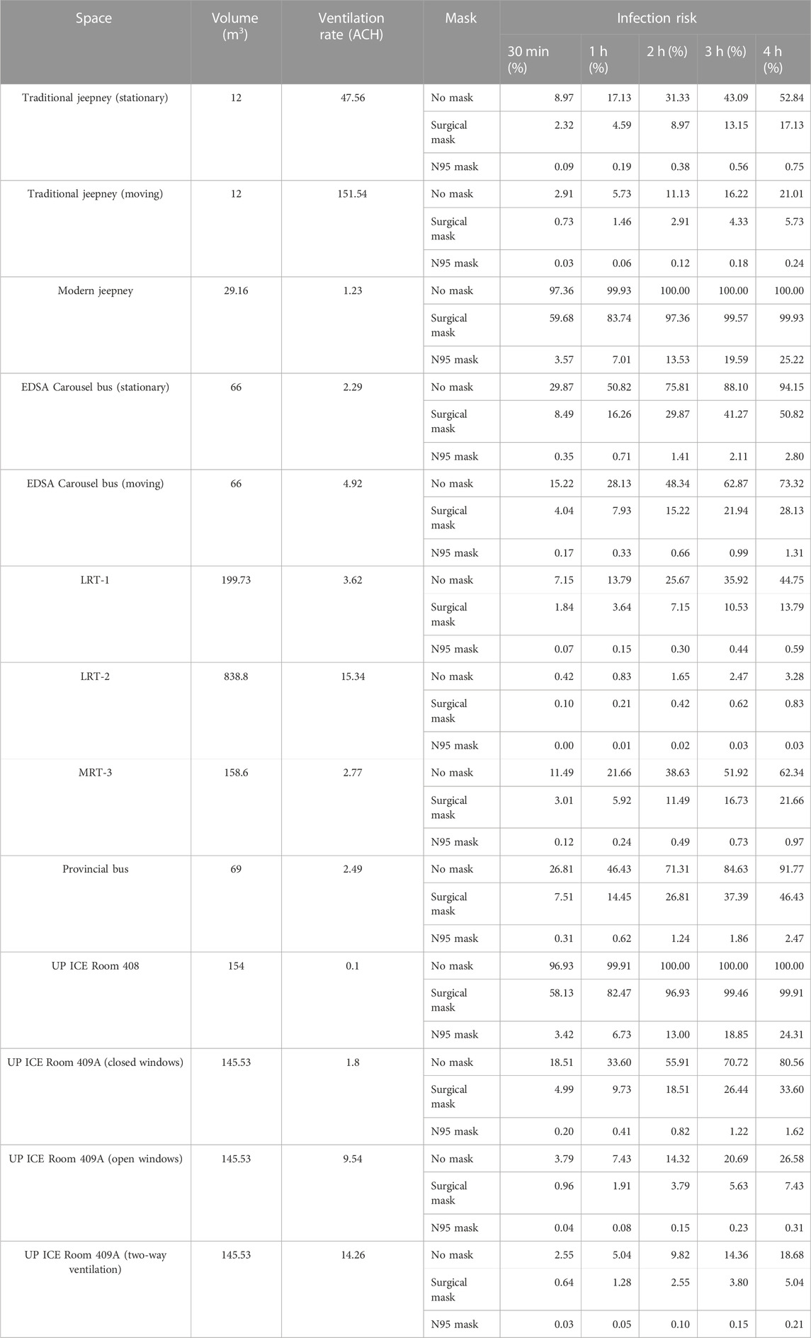
TABLE 1. Summary of infection risk due to the Alpha variant.
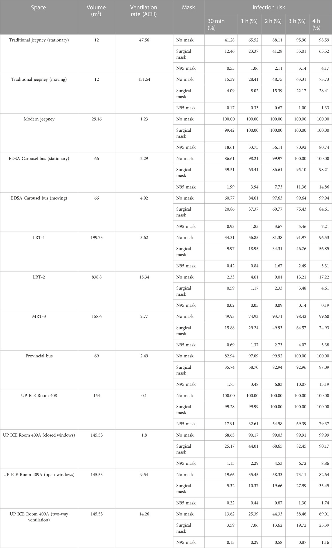
TABLE 2. Summary of infection risk due to the Delta variant.
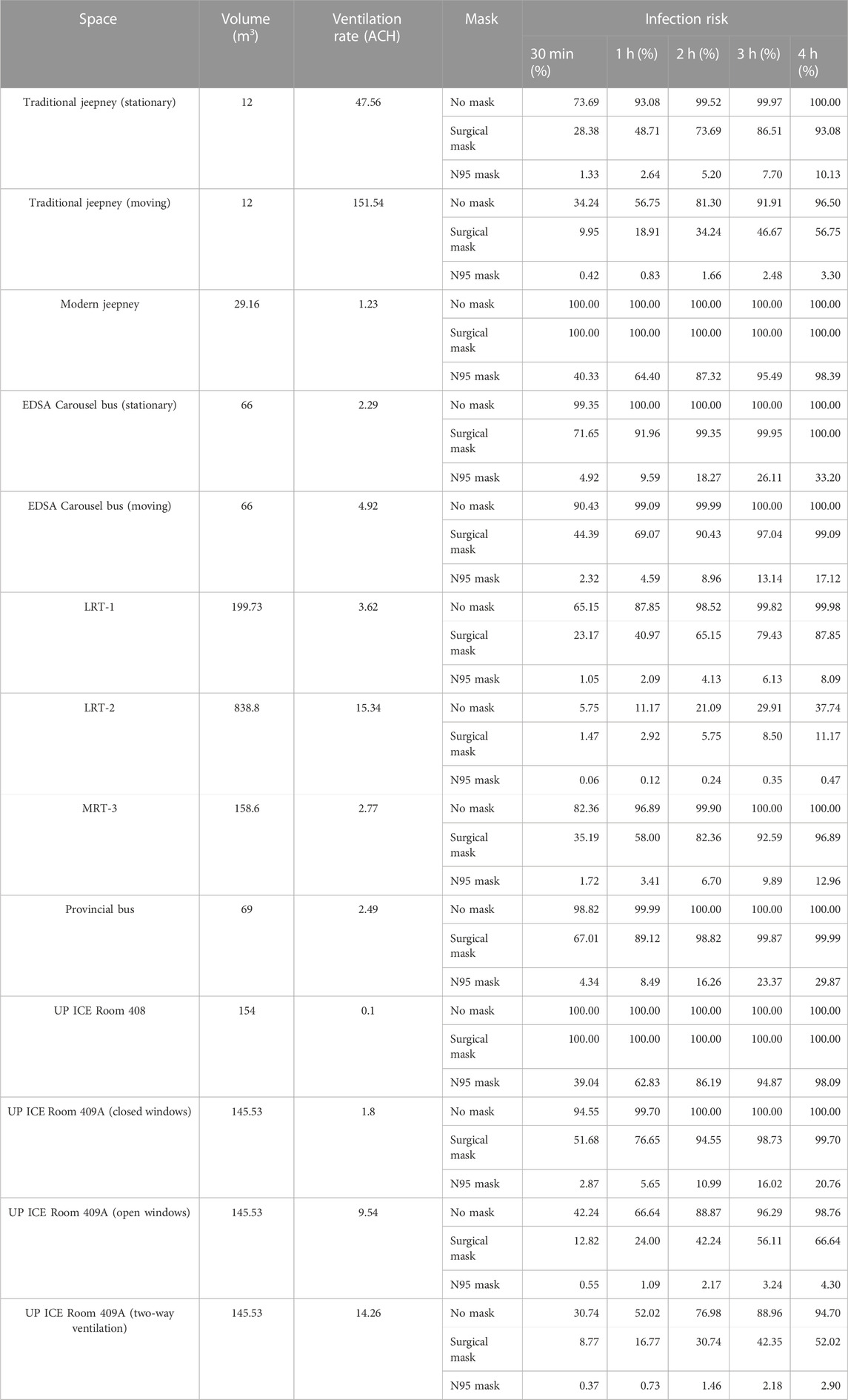
TABLE 3. Summary of infection risk due to the Omicron variant.
Due to the inverse relationship between ventilation rates and infection risks, infection risks are determined to be higher in indoor spaces with low ventilation rates. However, having high ventilation rates do not mean low infection risks as smaller spaces will also have higher infection risks. The computations also show that the better the quality of masks that were used, the lower the infection risk.
4 Conclusion and recommendations
The study developed an economical CO2 monitoring device that was deployed in various indoor spaces. The CO2 readings then undergo multivariate analysis using the least squares method to derive the ventilation rate and occupancy.
The method augments the limitation to the previous steady-state methods in deriving the ventilation rates; however, the method itself is incapable of deriving the ventilation rates and occupancy when the CO2 levels presume a steady-state condition. The method is also limited to increasing CO2 levels as it returns negative values when tested on decreasing CO2 levels. The method could also underestimate the occupancy if the activity rate of the occupants is less than the average.
To handle the limitations, an alternate method was used to derive the CO2 levels with the known number of occupants as an additional input. A camera-based people counter can be coupled to the CO2 monitor to accurately derive the ventilation rates. As to the activity rate, noise meters can be used to gauge human activity within the indoor facility, which can be related to the activity rates to adjust the parameters of the method.
The derived ventilation rates were then used to estimate the infection risk of different indoor spaces and public transportation modes. For most of the indoor spaces, the higher ventilation rates indicate lower risks, apart from traditional jeepneys which may have medium risk, especially if the jeepneys were stationary. Masking was also determined to have attributed to most infection risk reduction.
The developed CO2 monitors, which employ the multivariate method and the Wells–Riley formulations, can be a useful tool in informing occupants of the relative risk that they may be subjected to due to airborne diseases transmitted through shared room air transmission.
Data availability statement
The original contributions presented in the study are included in the article/Supplementary Material; further inquiries can be directed to the corresponding author.
Author contributions
JA: conceptualization, formal analysis, funding acquisition, investigation, methodology, project administration, visualization, and writing–original draft. JL: editing and revisions. PM: software and writing–review and editing. JH: resources, supervision, and writing–review and editing. JR: resources, supervision, and writing–review and editing.
Funding
The author(s) declare that financial support was received for the research, authorship, and/or publication of this article. The development of the CO2 monitors and part of this study are funded by the UPD OVCRD Extension Grant under (Project No. 222201 UPD-EG). This study is also funded by the DOST through the UP Center for Air Research in Urban Environments (UP CARE) research program.
Acknowledgments
The main author also acknowledges Dr. Jose Regin F. Regidor, the Director of the UPD Institute of Civil Engineering, who has been supportive of this initiative. The main author also acknowledges Dr. Ma. Antonia N. Tanchuling, the Dean of the UPD College of Engineering, for the endorsement and support. The authors acknowledge the Department of Transportation for allowing them to conduct CO2 measurements.
Conflict of interest
The authors declare that the research was conducted in the absence of any commercial or financial relationships that could be construed as a potential conflict of interest.
Publisher’s note
All claims expressed in this article are solely those of the authors and do not necessarily represent those of their affiliated organizations, or those of the publisher, the editors, and the reviewers. Any product that may be evaluated in this article, or claim that may be made by its manufacturer, is not guaranteed or endorsed by the publisher.
References
Bazant, M., Kodio, O., Cohen, A., Khan, K., Gu, Z., Bush, J. W. M., et al. (2021). Monitoring carbon dioxide to quantify the risk of indoor airborne transmission of COVID-19. doi:10.1017/flo.2021.10
Buonnano, G., Stabile, L., and Morawska, L. (2020). Estimation of airborne viral emission: quanta emission rate of SARS-CoV-2 for infection risk assessment. Environ. Int. 141, 105794. doi:10.1016/j.envint.2020.105794
Chen, W., Zhang, N., Wei, J., Yen, H. L., and Li, Y. (2020). Short-range airborne route dominates exposure of respiratory infection during close contact. Build. Environ. 176, 106859. doi:10.1016/j.buildenv.2020.106859
Dai, H., and Zhao, B. (2023). Association between the infection probability of COVID-19 and ventilation rates: an update for SARS-CoV-2 variants. Build. Simul. 6, 3–12. doi:10.1007/s12273-022-0952-6
Gammaitoni, L., and Nucci, M. C. (1997). Using a mathematical model to evaluate the efficacy of TB control measures. Emerg. Infect. Dis. 3, 335–342. doi:10.3201/eid0303.970310
Greenhalgh, T., Jimenez, J. L., Prather, K. A., Tufekci, Z., Fisman, D., and Schooley, R. (2021). Ten scientific reasons in support of airborne transmission of SARS-CoV-2. Lancet 397 (10285), 1603–1605. doi:10.1016/s0140-6736(21)00869-2
Jimenez, J. L., Marr, L. C., Randall, K., Ewing, E. T., Tufekci, Z., Greenhalgh, T., et al. (2022). What were the historical reasons for the resistance to recognizing airborne transmission during the COVID-19 pandemic? Indoor Air 32 (8), e13070. doi:10.1111/ina.13070
Klopmas, M., Milton, D. K., Ree, C., Baker, M. A., and Leekha, S. (2021). Current insights into respiratory virus transmission and potential implications for infection control programs: a narrative review. Ann. Intern. Med. 172 (12), 1710–1718. doi:10.7326/m21-2780
López, J. H., Romo, Á. S., Molina, D. C., Hernández, G. Á., Cureño, Á. B. G., Acosta, M. A., et al. (2021). Detection of Sars-Cov-2 in the air of two hospitals in Hermosillo, Sonora, México, utilizing a low-cost environmental monitoring system. Int. J. Infect. Dis. 102, 478–482. doi:10.1016/j.ijid.2020.10.089
Miller, S. L., Nazaroff, W. W., Jimenez, J. L., Boerstra, A., Buonanno, G., Dancer, S. J., et al. (2021). Transmission of SARS-CoV-2 by inhalation of respiratory aerosol in the Skagit Valley Chorale superspreading event. Indoor Air 31 (2), 314–323. doi:10.1111/ina.12751
Nissen, K., Krambrich, J., Akaberi, D., Hoffman, T., Ling, J., Lundkvist, Å., et al. (2020). Long-distance airborne dispersal of SARS-CoV-2 in COVID-19 wards. Sci. Rep. 10, 19589. doi:10.1038/s41598-020-76442-2
Peng, Z., and Jimenez, J. L. (2021). Exhaled CO2 as a COVID-19 infection risk proxy for different indoor environments and activities. Environ. Sci. Technol. 8 (5), 392–397. doi:10.1021/acs.estlett.1c00183
Peng, Z., Rojas, A. P., Kropff, E., Bahnfleth, W., Buonanno, G., Dancer, S., et al. (2022). Practical indicators for risk of airborne transmission in shared indoor environments and their application to COVID-19 outbreaks. Environ. Sci. Technol. 56 (2), 1125–1137. doi:10.1021/acs.est.1c06531
Persily, A., and de Jonge, L. (2018). Carbon dioxide generation rates for building occupants. Indoor Air 27 (5), 868–879. doi:10.1111/ina.12383
Qian, H., Miao, T., Liu, L., Zheng, X., Luo, D., and Li, Y. (2021). Indoor transmission of SARS-CoV-2. Indoor Air 31 (3), 639–645. doi:10.1111/ina.12766
Riley, E. C., Murphy, G., and Riley, R. L. (1978). Airborne spread of measles in a suburban elementary school. Am. J. Epidemiol. 107 (5), 421–432. doi:10.1093/oxfordjournals.aje.a112560
Rudnick, S., and Milton, D. (2003). Risk of indoor airborne infection transmission estimated from carbon dioxide concentration. Indoor Air 13 (3), 237–245. doi:10.1034/j.1600-0668.2003.00189.x
Shinohara, N., Sakaguchi, J., Kim, H., Kagi, N., Tatsu, K., Mano, H., et al. (2021). Survey of air exchange rates and evaluation of airborne infection risk of COVID-19 on commuter trains. Environ. Int. 157, 106774. doi:10.1016/j.envint.2021.106774
Wells, W. F. (1955). Airborne contagion and air hygiene. Cambridge, Massachussetts: Harvard University Press.
Keywords: indoor, air, ventilation, CO2, monitoring
Citation: Agar JC, Lustro JRT, Magpantay P, Hizon JRE and Reyes JGT (2023) Ventilation and disease monitoring of indoor spaces and public transportation using an NDIR sensor network. Front. Built Environ. 9:1306072. doi: 10.3389/fbuil.2023.1306072
Received: 03 October 2023; Accepted: 27 November 2023;
Published: 19 December 2023.
Edited by:
Asit Kumar Mishra, University of Galway, IrelandReviewed by:
Andrea Frattolillo, University of Cagliari, ItalyJiayu Li, University of California, Berkeley, Singapore
Copyright © 2023 Agar, Lustro, Magpantay, Hizon and Reyes. This is an open-access article distributed under the terms of the Creative Commons Attribution License (CC BY). The use, distribution or reproduction in other forums is permitted, provided the original author(s) and the copyright owner(s) are credited and that the original publication in this journal is cited, in accordance with accepted academic practice. No use, distribution or reproduction is permitted which does not comply with these terms.
*Correspondence: Joshua C. Agar, amNhZ2FyQHVwLmVkdS5waA==