 Santiago Ruiz
 Wei Song
- Department of Civil, Construction and Environmental Engineering, The University of Alabama, Tuscaloosa, AL, United States
For Real-time hybrid simulation (RTHS) to be stable and accurate, it is essential to address the time desynchronization issue between the numerical and physical substructures. Desynchronization is primarily caused by time delays, inherent dynamics of the control plant, system uncertainties, and noises. While existing adaptive compensators have shown effective tracking performance in single-input single-output (SISO) RTHS, their effectiveness in multi-input multi-output (MIMO) RTHS has not been fully demonstrated. MIMO-RTHS presents additional challenges due to its larger solution space, and significant dynamic coupling between actuators. To address these challenges, this study introduces an adaptive compensation framework for MIMO-RTHS. The proposed framework utilizes a control law based on the inverse dynamics of the control plant, incorporating real-time adaptive parameter updates through Extended Kalman Filter (EKF) and Unscented Kalman Filter (UKF) methods. Both the transfer function (TF) and discrete-time state-space (SS) models of the plant are employed in distinct parameter estimation cases. The performance of the proposed compensation is validated through a multi-axial RTHS (maRTHS) benchmark problem. Extensive simulations on the maRTHS incorporating various earthquake inputs, sensor noise, and model uncertainties, demonstrated an excellent tracking performance and strong robustness across four parameter estimation cases (EKF-TF, UKF-TF, EKF-SS, and UKF-SS). The use of UKF with SS model (UKF-SS) achieved superior performance, effectively managing nonlinearities and noise without requiring low-pass filtering.
1 Introduction
Real-time hybrid simulation (RTHS) is an experimental technique to perform dynamic evaluation of complex structural systems (Nakashima et al., 1992). This technique divides the emulated structure into two parts: the numerical substructure (NS), which is simulated by a computer program, and the physical substructure (PS), which is tested in a laboratory. The interface between the NS and the PS is imposed by a transfer system (e.g., servo hydraulic actuator) in real-time. The transfer system along with the PS is often refer to as the control plant. While RTHS offers a cost-effective and spatially economical alternative to traditional structural tests (Gomez et al., 2014), it faces a critical issue of desynchronization at the NS-PS interface. This issue can cause significant experimental errors or even failure, impacting the accuracy and stability of RTHS (Darby et al., 1999; Horiuchi et al., 1999; Zhao et al., 2003). A primary cause of desynchronization is “actuator time delay” or simply “time delay”, which originates from the closed-loop nature of RTHS, inherent dynamics of the control plant, and data acquisition limitations (Hayati and Song, 2017; Hayati and Song, 2018). This issue is further exacerbated by system modeling uncertainties (Silva et al., 2020), and process and measurement noises (Song and Dyke, 2013; Song, 2018; Song et al., 2020).
To mitigate the desynchronization issue, numerous compensation strategies have been developed. Traditional strategies assume constant time delay and rely on pre-estimations of system parameters. These strategies include polynomial extrapolation (Horiuchi et al., 1999; Nakashima and Masaoka, 1999; Darby et al., 2002), phase lead compensation (Zhao et al., 2003; Jung et al., 2007), and inverse compensation (Chen et al., 2009; Chen and Ricles, 2009). However, in RTHS, time delays are not constant due to frequency-dependent uncertainties in actuator dynamics and specimen characteristics (Dyke et al., 1995; Darby et al., 2002; Hayati and Song, 2017; Hayati and Song, 2018). Consequently, traditional compensation strategies fall short when dealing with significant system uncertainties (Silva et al., 2020; Condori Uribe et al., 2023). Recently, adaptive compensation strategies have gained considerable attention due to their ability to dynamically adjust their parameters in real-time, responding to changes and uncertainties in the system (Chae et al., 2013; Chen et al., 2015; Ouyang et al., 2019).
Parameter estimation method is a popular and effective adaptive control approach, and it has already been introduced into RTHS compensation domain. Chae et al. (2013) developed the adaptive time series (ATS) compensation, which updates the coefficients of a transfer system using the least squares (LS) method for single-input single-output (SISO) RTHS. Palacio-Betancur and Gutierrez Soto (2019) extended this method by implementing recursive least squares (RLS) for parameter estimation in SISO-RTHS. Further studies by Wang et al. (2020) and Ning et al. (2022) explored adaptive control schemes for SISO-RTHS based on discrete system models with time-varying coefficients using the LS method, while Ning et al. (2020) implemented Kalman filter (KF) as the parameter estimator. To enhance the robustness of adaptive control in SISO-RTHS, nonlinear parameter estimators, such as the Extended Kalman Filter (EKF) and Unscented Kalman Filter (UKF) have been employed. The EKF linearizes the system around the current estimate to handle nonlinearities, while the UKF uses a deterministic sampling approach to capture the mean and covariance more accurately (Wan and Van Der Merwe, 2000). The computational efficiency, ability to provide timely updates, and robustness against nonlinearities and noises of EKF and UKF, make these estimators suitable for real-time nonlinear model updating (Song and Dyke, 2013; Song and Dyke, 2014). Strano and Terzo (2016) developed an adaptive compensation scheme based on EKF, to continuously adjust system parameters, enhancing the accuracy and stability of hydraulic actuator control in RTHS. Huang et al. (2023) and Wang et al. (2024) investigated adaptive compensation with UKF, exhibiting good robustness.
Despite the demonstrated effectiveness of adaptive control using nonlinear parameter estimation methods in SISO-RTHS, its application to multi-input multi-output (MIMO) RTHS remains unverified. The transition from SISO- to MIMO-RTHS enables the simulation of more realistic loading scenarios and complex structural responses; however, it introduces unique challenges. In MIMO-RTHS, control actions applied to one actuator can affect responses in other actuators due to interdependencies across the MIMO control plant, creating cross-coupling effects that prevent the direct application of existing SISO strategies. Furthermore, the development of MIMO-RTHS involves a higher level of complexities than the SISO counterparts, including a larger and more intricate solution space, complex actuator kinematics, and increased computational demand (Mercan et al., 2009; Condori Uribe et al., 2023; Najafi et al., 2023). To address these challenges and achieve effective compensation, this study presents a robust adaptive compensation strategy for MIMO-RTHS, validated through a multi-axial RTHS (maRTHS) benchmark problem (Condori Uribe et al., 2023). The contributions of this work are twofold: (i) the development of a comprehensive adaptive compensation framework based on nonlinear parameter estimations (EKF and UKF), which provides a systematic approach for MIMO-RTHS; (ii) the system formulation for parameter estimation, which considers the control plant in two commonly-adopted dynamic system models, namely the transfer function (TF) and the discrete-time state-space (SS) models, resulting in four distinct parameter estimation cases: EKF-TF, UKF-TF, EKF-SS, and UKF-SS. The proposed framework allows for implementation flexibility and performance comparison among the different estimation techniques and system formulations. Through a comparative study using the maRTHS benchmark problem (Condori Uribe et al., 2023), it is shown that the proposed compensation framework can account for the interactions and dependencies between multiple inputs and outputs, effectively managing the dynamic coupling between actuators during MIMO-RTHS.
The remainder of this paper is organized as follows. Section 2 presents the proposed adaptive compensation methodology. Section 3 details the implementation and results of the virtual maRTHS. Finally, Section 4 summarizes the main findings and conclusions of this research.
2 Methodology
In this section, the proposed adaptive compensation framework for MIMO-RTHS is presented, to mitigate the desynchronization between the NS and PS, such that the output of the control plant tracks the “desired” (or “target”) signals. This compensator employs a control law based on the inverse dynamics of the control plant, which aims to cancel the plant dynamics. Thus, the control plant model is a key aspect for the formulation of the presented methodology. This work explores two distinct models of the control plant: (a) a transfer function model; (b) a discrete-time state-space model. Both models are utilized for parameter estimation in distinct cases. However, only the transfer function model is used during the command generation (control law).
2.1 Control plant
2.1.1 Transfer function model
The control plant that comprises the PS in a MIMO problem can be generally represented by a matrix of transfer functions (TFs) as,
where
where
In this work, the zeros and poles from Equation 2 are expressed as a parameter vector,
2.1.2 Discrete-time state-space model
The identified transfer function of the plant from Equation 1 can be used to obtain a state-space (SS) realization in discrete time as,
where
2.2 Adaptive compensation framework
While adaptive control schemes have been developed for SISO-RTHS (e.g., Strano and Terzo (2016), Huang et al. (2023)), they have yet to be applied in MIMO-RTHS. In this work, the proposed adaptive compensation framework is realized for coupled MIMO systems, such as those presented in Equations 1–4, accounting for system uncertainties (
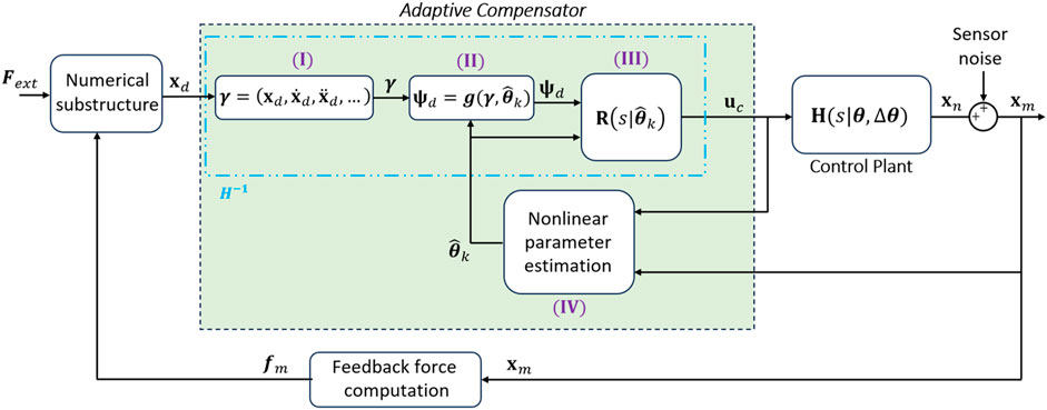
Figure 1. maRTHS scheme and proposed adaptive compensator.
The collection of blocks (I), (II), and (III) in Figure 1 generates the control law, which is realized by utilizing the inverse dynamics of the control plant derived from the transfer function in Equation 1. The control law incorporates adaptive parameters that are estimated by block (IV) at each time step. The parameter estimation process is described in Section 2.3. The remainder of this section explains the control generation process.
The transfer function matrices
where
where
where
The presented approach addresses the issue of improper transfer functions in
2.3 Nonlinear parameter estimation
The physical domain of RTHS is subject to disturbances such as imprecisions in experimental setup, unmodeled process and dynamics (e.g., friction), and process and measurement noises, which introduce uncertainties to the plant (
Both EKF and UKF are formulated for a general discrete-time system model expressed as,
where
Depending on the plant model employed for the application of EKF or UKF, the corresponding estimation system models are explained below.
a) Transfer function model
For the control plant in transfer function (TF) form, the state vector and process function at time step
The observation function is set as the command signal
In this formulation, the nonlinearity arises from Equation 12, where the computation of the system output vector
b) Discrete-time state-space model
When the discrete-time state-space (SS) model of the control plant is used for parameter estimation, the original states of the system from Equations 3, 4 are augmented with the parameters that need to be estimated. Thus, the state transition and observation functions for the augmented discrete-time SS model are formulated as,
where
where
Regardless of the selected system model (TF or SS), both EKF and UKF can be applied for parameter estimation. The estimation methods are depicted in Figure 2 utilizing the general system formulation of Equations 9, 10.
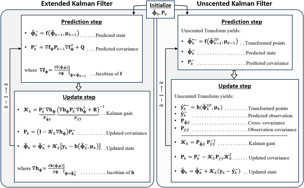
Figure 2. EKF and UKF state estimation.
EKF and UKF are extensions of the standard Kalman filter, designed to handle nonlinear systems (Song, 2011). Both methods consist of two recursive steps: the prediction step and the update step, as shown in Figure 2. In the prediction step, the process function
The primary difference between these estimation methods lies in handling the nonlinearities of the process and observation functions. The EKF approximates the nonlinear functions by linearizing them around the current state estimate using a first-order Taylor series expansion, which involves calculating their respective Jacobians
By replacing the general system formulation of Equations 9, 10 in Figure 2 with the selected control plant formulations from Equations 11, 12 (for the TF model) or Equations 13, 14 (for the discrete-time SS model), four (4) parameter estimation cases can be obtained: EKF-TF, UKF-TF, EKF-SS, and UKF-SS. These cases are illustrated in Figure 3, showing the architecture inside of block IV from Figure 1.
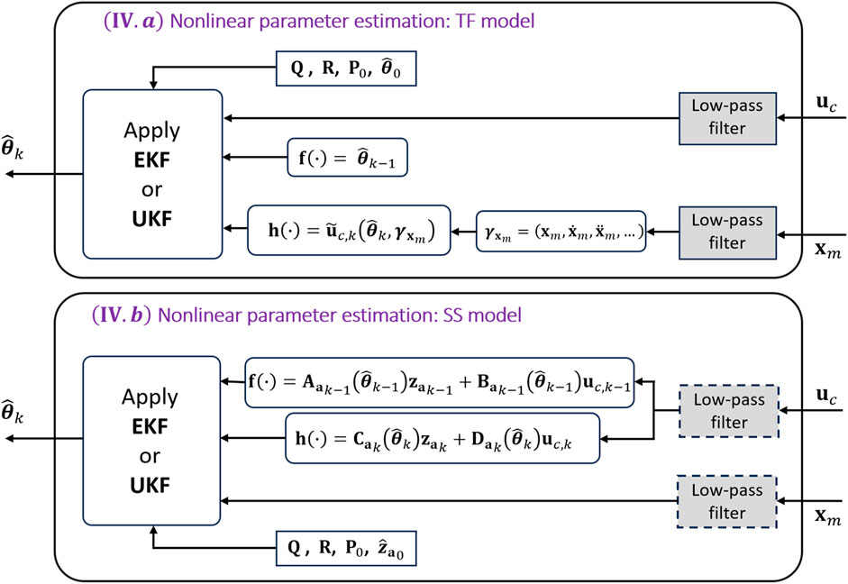
Figure 3. maRTHS nonlinear parameter estimation cases.
As shown in Figure 3, the same low-pass filter is applied to the signals
3 Results
3.1 maRTHS benchmark problem
The proposed methodology is applied to the maRTHS benchmark developed by Condori Uribe et al. (2023), which provides a virtual RTHS (vRTHS) platform that allows the implementation of customized compensators. In this benchmark problem a three-story, three-bay moment resisting frame is subjected to seismic base excitation corresponding to scaled ground acceleration records of El Centro 1940, Kobe 1995, and Morgan Hill 1984. The central frame of the structure (one-story, one-bay, simply supported) acts as the experimental substructure (see Figure 4), and the remaining structure is the numerical substructure. Displacement and rotational degrees of freedom (DOFs) are used as target signals at the NS-PS interface (control node). These DOFs are refer to as “frame coordinates”, and are represented in Figure 4 as
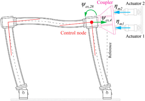
Figure 4. Experimental substructure. Adapted from Condori Uribe et al. (2023).
In this work, the compensation is performed in the actuator coordinates domain. Therefore, the desired signal is specified as
The control plant model for the maRTHS benchmark problem is given as Equation 19,
where the subscripts represent the input-output pairs for actuator 1 and actuator 2, respectively. Specifically,
From Equations 20–23,
3.2 Parameter estimation settings
The parameters in Equations 20–23 are updated in real-time during RTHS, while the transfer function gains are considered as constants. This approach results in the definition of
Once the control plant model
As indicated in Section 2.3, a search process is performed to select the initial values of
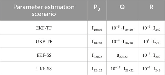
Table 1. Tuned EKF and UKF parameters for maRTHS Benchmark Problem.
In addition to the covariances presented in Table 1, scaling parameters used during the sigma points computation in UKF were adjusted to enhance the estimation performance. The values for these scaling parameters are set as follows:
3.3 Adaptive compensator performance in maRTHS
The proposed adaptive compensator is validated through the vRTHS platform in MATLAB/Simulink R2023b (Mathworks, 2024). The performance is evaluated with a set of 10 performance criteria defined in Condori Uribe et al. (2023). Performance indices (PI),
A total of 1,000 vRTHS simulations were executed to demonstrate the control robustness, each incorporating system uncertainties (
The mean and standard deviation (SD) for each performance indicator (PI) across the four parameter estimation cases using 0.4 scaled El Centro Earthquake as input, are presented in Table 2. Additionally, the results from the linear quadratic regulator (LQR) controller presented in the benchmark (BM) by Condori Uribe et al. (2023) are included in the table for comparison. Results utilizing 0.4 scaled Kobe and 0.4 scaled Morgan earthquakes are presented in the Supplementary Material. Furthermore, Table 3 presents the average simulation time for each earthquake input to evaluate computational efficiency.
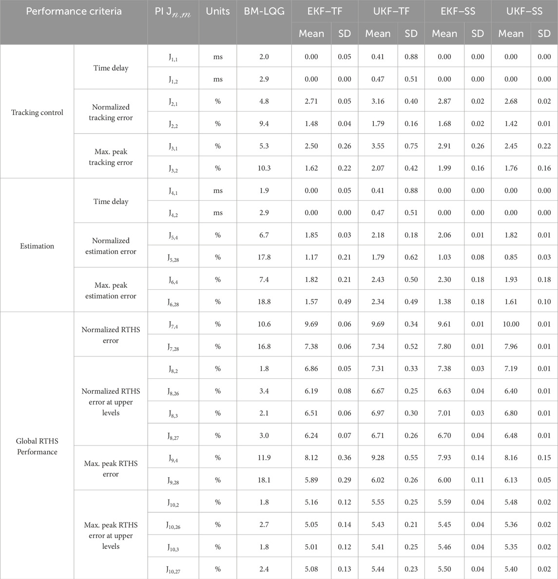
Table 2. Evaluation criteria of maRTHS subjected to 0.4 scaled El Centro Earthquake (1,000 simulations).

Table 3. Average simulation time for each earthquake input case (1,000 simulations).
The results from Table 2 demonstrate the effectiveness and robustness of the parameter estimation cases for the proposed compensator using the 0.4 scaled El Centro Earthquake as input. The robustness is confirmed by the performance across the 1,000 simulations, which resulted in small PIs with small standard deviations. For time delay, all cases were effective, with the highest mean time delay of
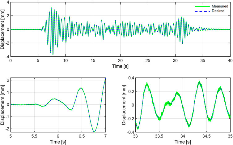
Figure 5. maRTHS tracking performance in actuator coordinates (actuator 1) for UKF-SS case with the largest
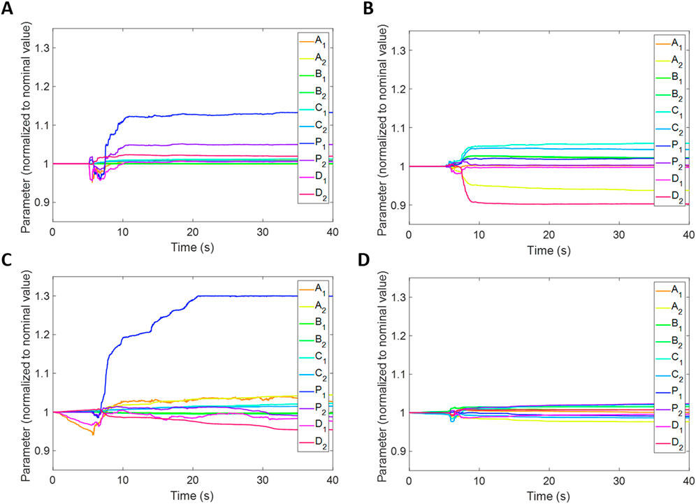
Figure 6. Parameter tracking with 0.4 scaled El Centro Earthquake as input and control plant with uncertainties. (A) EKF-SS (B) UKF-SS. (C) EKF-TF (D) UKF-TF.
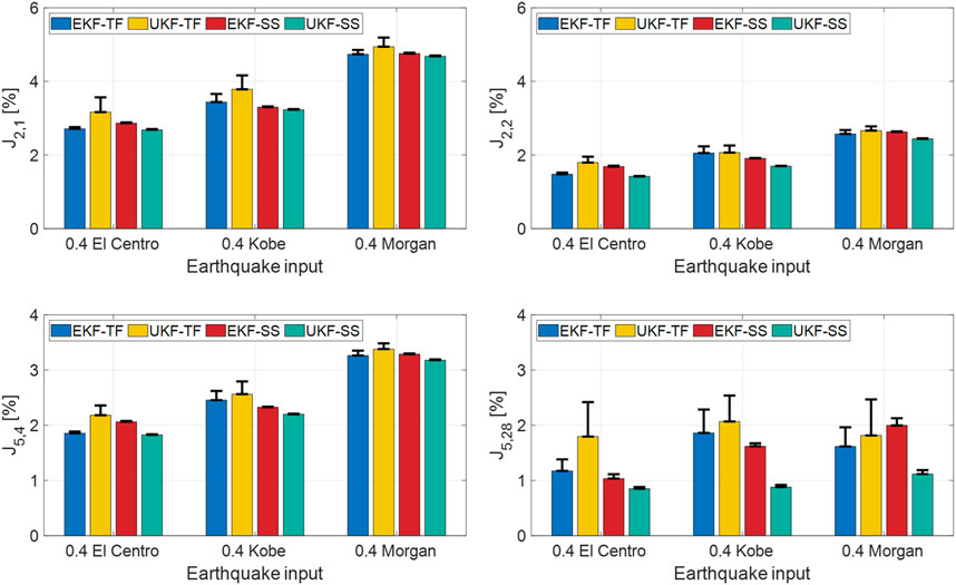
Figure 7. Tracking performance in actuator and frame coordinates for all input earthquakes. Mean PIs obtained from 1,000 simulations for each earthquake input.
Although the UKF-SS shows superior tracking performance compared to the other cases studied, it is also more computationally expensive, as shown in Table 3. This increased computational cost is likely due to the requirement for the UKF algorithm to generate and propagate multiple sigma points, which involves additional matrix operations. Note that, the simulation time indicated in Table 3 is measured during the numerical simulations in MATLAB under Windows environment, not in a real-time computing environment. But by considering the same computational environment, Table 3 can still offer a relative comparison of the computational efficiency of each algorithm.
3.4 Effect of low-pass filter in state-space formulation
Results presented in Section 3.3 are obtained with the use of a 6th-order Butterworth low-pass filter with a cutoff frequency of 20 Hz, applied to
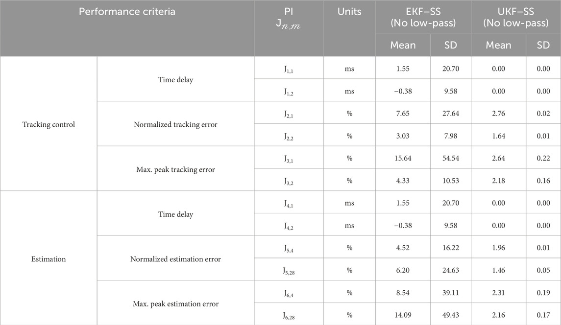
Table 4. Tracking performance criteria of maRTHS subjected to 0.4 scaled El Centro Earthquake (1,000 simulations)–SS formulation without low-pass filter.
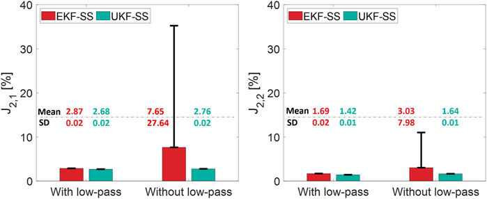
Figure 8. Tracking performance criteria for EKF-SS and UKF-SS with and without low-pass filtering.
These results reveal that UKF can handle noises and nonlinearities in the system model more effectively than EKF when low-pass filter is not present. This capability is advantageous in RTHS because the use of low-pass filter can potentially introduce signal distortion leading to unwanted dynamics with potentially nonlinear systems, and therefore compromise the compensation performance and the accuracy of the simulated response.
4 Conclusion
An adaptive compensation framework for MIMO-RTHS is proposed in this paper. The proposed methodology employs a control law based on the inverse dynamics of the control plant, with adaptive parameters updated in real-time. Parameter estimation utilizes the plant model in TF and discrete-time SS forms, combined with nonlinear parameter estimators EKF and UKF, leading to four proposed estimation cases: EKF-TF, UKF-TF, EKF-SS, and UKF-SS.
The proposed compensation has been examined in a maRTHS benchmark problem, through RTHS simulations incorporating sensor noise, uncertainties in the plant model, and three earthquake inputs. The results for the four parameter estimation cases of the proposed compensation framework showed effective tracking performance at the NS-PS interface node in both actuator and frame coordinates, and strong robustness against uncertainties and noises, with the UKF-SS case exhibiting the best performance in compensation tracking (see Table 2; Figure 7) and robustness against uncertainties and noises (see Table 4; Figure 8). From the implementation of the proposed adaptive compensation, the following additional observations are listed:
• EKF exhibits a higher computational efficiency than UKF, which is reflected by the shorter simulation times of EKF-TF and EFK-SS cases in comparison to UKF-TF and UKF-SS cases (see Table 3). The higher computational complexity of the UKF might pose a challenge in meeting real-time constraints. Therefore, based on the results from Table 3, the EKF-SS case is an efficient choice when the system does not exhibit nonlinearities.
• Utilizing the TF model for parameter estimation (cases EKF-TF and UKF-TF) resulted in a smaller solution space compared to the SS model, but its implementation was more computationally expensive because of the calculations of time derivatives, as indicated by
• From the results in Section 3.4, it is shown that the UKF-SS case maintains good tracking performance without the need of low-pass filtering. Therefore, when RTHS system exhibits strong nonlinearities where low-pass filtering is not suitable, the UKF-SS is the preferred choice due to its robust tracking performance against uncertainties and noises with or without low-pass filtering.
• The implementation of EKF was more involved than UKF, because the high nonlinearity in the system formulations (see Section 2.3) makes the derivation of the Jacobians cumbersome and prone to errors.
The proposed adaptive compensation framework shows significant potential for tracking performance and robustness in MIMO-RTHS. Future research will focus on strengthening the efficiency and robustness of this framework by investigating alternative system formulations and exploring more advanced parameter estimation methods.
Data availability statement
The raw data supporting the conclusions of this article will be made available by the authors, without undue reservation.
Author contributions
SR: Methodology, Data curation, Formal Analysis, Investigation, Software, Visualization, Writing–original draft. WS: Methodology, Conceptualization, Funding acquisition, Project administration, Resources, Supervision, Validation, Writing–review and editing.
Funding
The author(s) declare that financial support was received for the research, authorship, and/or publication of this article. This research was supported by National Science Foundation (NSF) through Grant CMMI 2011423.
Conflict of interest
The authors declare that the research was conducted in the absence of any commercial or financial relationships that could be construed as a potential conflict of interest.
The author(s) declared that they were an editorial board member of Frontiers, at the time of submission. This had no impact on the peer review process and the final decision.
Publisher’s note
All claims expressed in this article are solely those of the authors and do not necessarily represent those of their affiliated organizations, or those of the publisher, the editors and the reviewers. Any product that may be evaluated in this article, or claim that may be made by its manufacturer, is not guaranteed or endorsed by the publisher.
Supplementary material
The Supplementary Material for this article can be found online at: https://www.frontiersin.org/articles/10.3389/fbuil.2024.1477804/full#supplementary-material
References
Carrion, J. E., Spencer, B. F., and Phillips, B. M. (2009). Real-time hybrid simulation for structural control performance assessment. Earthq. Eng. Eng. Vib. 8, 481–492. doi:10.1007/s11803-009-9122-4
Chae, Y., Kazemibidokhti, K., and Ricles, J. M. (2013). Adaptive time series compensator for delay compensation of servo-hydraulic actuator systems for real-time hybrid simulation. Earthq. Eng. Struct. Dyn. 42, 1697–1715. doi:10.1002/eqe.2294
Chen, C., and Ricles, J. M. (2009). Analysis of actuator delay compensation methods for real-time testing. Eng. Struct. 31, 2643–2655. doi:10.1016/j.engstruct.2009.06.012
Chen, C., Ricles, J. M., Marullo, T. M., and Mercan, O. (2009). Real-time hybrid testing using the unconditionally stable explicit CR integration algorithm. Earthq. Eng. Struct. Dyn. 38, 23–44. doi:10.1002/eqe.838
Chen, P.-C., Chang, C.-M., Spencer, B. F., and Tsai, K.-C. (2015). Adaptive model-based tracking control for real-time hybrid simulation. Bull. Earthq. Eng. 13, 1633–1653. doi:10.1007/s10518-014-9681-2
Condori Uribe, J. W., Salmeron, M., Patino, E., Montoya, H., Dyke, S. J., Silva, C. E., et al. (2023). Experimental benchmark control problem for multi-axial real-time hybrid simulation. Front. Built Environ. 9, 1270996. doi:10.3389/fbuil.2023.1270996
Darby, A. P., Blakeborough, A., and Williams, M. S. (1999). Real-time substructure tests using hydraulic actuator. J. Eng. Mech. 125, 1133–1139. doi:10.1061/(ASCE)0733-9399(1999)125:10(1133)
Darby, A. P., Williams, M. S., and Blakeborough, A. (2002). Stability and delay compensation for real-time substructure testing. J. Eng. Mech. 128, 1276–1284. doi:10.1061/(ASCE)0733-9399(2002)128:12(1276)
Dyke, S. J., Spencer, B. F., Quast, P., and Sain, M. K. (1995). Role of control-structure interaction in protective system design. J. Eng. Mech. 121, 322–338. doi:10.1061/(ASCE)0733-9399(1995)121:2(322)
Gomez, D., Dyke, S., and Maghareh, A. (2014). Enabling role of hybrid simulation within the NEES infrastructure in advancing earthquake engineering practice and research. doi:10.13140/2.1.1828.6886
Hayati, S., and Song, W. (2017). An optimal discrete-time feedforward compensator for real-time hybrid simulation. Smart Struct. Syst. 20, 483–498. doi:10.12989/SSS.2017.20.4.483
Hayati, S., and Song, W. (2018). Design and performance evaluation of an optimal discrete-time feedforward controller for servo-hydraulic compensation. J. Eng. Mech. 144, 04017163. doi:10.1061/(ASCE)EM.1943-7889.0001399
Horiuchi, T., Inoue, M., Konno, T., and Namita, Y. (1999). Real-time hybrid experimental system with actuator delay compensation and its application to a piping system with energy absorber. Earthq. Eng. Struct. Dyn. 28, 1121–1141. doi:10.1002/(SICI)1096-9845(199910)28:10<1121::AID-EQE858>3.0.CO;2-O
Huang, W., Ning, X., Ding, Y., and Wang, Z. (2023). A novel actuation dynamics adaptive compensation strategy for real-time hybrid simulation based on unscented kalman filter. Int. J. Struct. Stab. Dyn. 23, 2350107. doi:10.1142/S0219455423501079
Julier, S. J. (2002). “The scaled unscented transformation,” in Proceedings of the 2002 American Control Conference (IEEE Cat. No.CH37301). Presented at the Proceedings of 2002 American Control Conference, Anchorage, AK, USA, 08-10 May 2002 (IEEE), 4555–4559. doi:10.1109/ACC.2002.1025369
Jung, R.-Y., Benson Shing, P., Stauffer, E., and Thoen, B. (2007). Performance of a real-time pseudodynamic test system considering nonlinear structural response. Earthq. Eng. Struct. Dyn. 36, 1785–1809. doi:10.1002/eqe.722
Mathworks (2024). MATLAB. Available at: https://www.mathworks.com/products/matlab.html (Accessed July 27, 2024).
Mercan, O., Ricles, J. M., Sause, R., and Marullo, T. (2009). Kinematic transformations for planar multi-directional pseudodynamic testing. Earthq. Eng. Struct. Dyn. 38, 1093–1119. doi:10.1002/eqe.886
Najafi, A., Fermandois, G. A., Dyke, S. J., and Spencer, B. F. (2023). Hybrid simulation with multiple actuators: a state-of-the-art review. Eng. Struct. 276, 115284. doi:10.1016/j.engstruct.2022.115284
Nakashima, M., Kato, H., and Takaoka, E. (1992). Development of real-time pseudo dynamic testing. Earthq. Eng. Struct. Dyn. 21, 79–92. doi:10.1002/eqe.4290210106
Nakashima, M., and Masaoka, N. (1999). Real-time on-line test for MDOF systems. Earthq. Eng. Struct. Dyn. 28, 393–420. doi:10.1002/(SICI)1096-9845(199904)28:4<393::AID-EQE823>3.0.CO;2-C
Ning, X., Wang, Z., Wang, C., and Wu, B. (2022). Adaptive feedforward and feedback compensation method for real-time hybrid simulation based on a discrete physical testing system model. J. Earthq. Eng. 26, 3841–3863. doi:10.1080/13632469.2020.1823912
Ning, X., Wang, Z., and Wu, B. (2020). Kalman filter-based adaptive delay compensation for benchmark problem in real-time hybrid simulation. Appl. Sci. 10, 7101. doi:10.3390/app10207101
Ouyang, Y., Shi, W., Shan, J., and Spencer, B. F. (2019). Backstepping adaptive control for real-time hybrid simulation including servo-hydraulic dynamics. Mech. Syst. Signal Process. 130, 732–754. doi:10.1016/j.ymssp.2019.05.042
Palacio-Betancur, A., and Gutierrez Soto, M. (2019). Adaptive tracking control for real-time hybrid simulation of structures subjected to seismic loading. Mech. Syst. Signal Process. 134, 106345. doi:10.1016/j.ymssp.2019.106345
Phillips, B. M., Takada, S., Spencer, B. F., and Fujino, Y. (2014). Feedforward actuator controller development using the backward-difference method for real-time hybrid simulation. Smart Struct. Syst. 14, 1081–1103. doi:10.12989/sss.2014.14.6.1081
Silva, C. E., Gomez, D., Maghareh, A., Dyke, S. J., and Spencer, B. F. (2020). Benchmark control problem for real-time hybrid simulation. Mech. Syst. Signal Process. 135, 106381. doi:10.1016/j.ymssp.2019.106381
Song, W. (2011). Dynamic model updating with applications in structural and damping systems: from linear to nonlinear, from off-line to real-time. PhD Thesis.
Song, W. (2018). Generalized minimum variance unbiased joint input-state estimation and its unscented scheme for dynamic systems with direct feedthrough. Mech. Syst. Signal Process. 99, 886–920. doi:10.1016/j.ymssp.2017.06.032
Song, W., and Dyke, S. (2013). Development of a cyber-physical experimental platform for real-time dynamic model updating. Mech. Syst. Signal Process. 37, 388–402. doi:10.1016/j.ymssp.2012.12.007
Song, W., and Dyke, S. (2014). Real-time dynamic model updating of a hysteretic structural system. J. Struct. Eng. 140, 04013082. doi:10.1061/(ASCE)ST.1943-541X.0000857
Song, W., Hayati, S., and Zhou, S. (2017). Real-time model updating for magnetorheological damper identification: an experimental study. Smart Struct. Syst. 20, 619–636. doi:10.12989/SSS.2017.20.5.619
Song, W., Sun, C., Zuo, Y., Jahangiri, V., Lu, Y., and Han, Q. (2020). Conceptual study of a real-time hybrid simulation framework for monopile offshore wind turbines under wind and wave loads. Front. Built Environ. 6, 129. doi:10.3389/fbuil.2020.00129
Strano, S., and Terzo, M. (2016). Actuator dynamics compensation for real-time hybrid simulation: an adaptive approach by means of a nonlinear estimator. Nonlinear Dyn. 85, 2353–2368. doi:10.1007/s11071-016-2831-0
Wan, E. A., and Van Der Merwe, R. (2000). “The unscented Kalman filter for nonlinear estimation,” in Proceedings of the IEEE 2000 Adaptive Systems for Signal Processing, Communications, and Control Symposium (Cat. No.00EX373). Presented at the Symposium on Adaptive Systems for Signal Processing Communications and Control, Lake Louise, Alta., Canada, 04-04 October 2000 (IEEE), 153–158. doi:10.1109/ASSPCC.2000.882463
Wang, T., Gong, Y., Xu, G., and Wang, Z. (2024). Unscented kalman filter-based two-stage adaptive compensation method for real-time hybrid simulation. J. Earthq. Eng. 28, 3221–3255. doi:10.1080/13632469.2024.2335346
Wang, Z., Guoshan, X., Qiang, L., and Bin, W. (2020). An adaptive delay compensation method based on a discrete system model for real-time hybrid simulation. SMART Struct. Syst. doi:10.12989/sss.2020.25.5.569
Keywords: real-time hybrid simulation, MIMO control, adaptive compensation, actuator tracking, uncertainty, hydraulic actuator, extended Kalman filter, unscented Kalman filter
Citation: Ruiz S and Song W (2024) Adaptive compensation for multi-axial real-time hybrid simulation via nonlinear parameter estimation. Front. Built Environ. 10:1477804. doi: 10.3389/fbuil.2024.1477804
Received: 08 August 2024; Accepted: 26 November 2024;
Published: 17 December 2024.
Edited by:
Cheng Fang, Tongji University, ChinaReviewed by:
James Michael Ricles, Lehigh University, United StatesBaiping Dong, Tongji University, China
Copyright © 2024 Ruiz and Song. This is an open-access article distributed under the terms of the Creative Commons Attribution License (CC BY). The use, distribution or reproduction in other forums is permitted, provided the original author(s) and the copyright owner(s) are credited and that the original publication in this journal is cited, in accordance with accepted academic practice. No use, distribution or reproduction is permitted which does not comply with these terms.
*Correspondence: Wei Song, d3NvbmdAZW5nLnVhLmVkdQ==