 Jin Terng Ma
 Luke Lapira
 M. Ahmer Wadee
- 1Department of Civil and Environmental Engineering, Imperial College London, London, United Kingdom
- 2Department of Civil, Environmental and Geomatic Engineering, University College London, London, United Kingdom
Beam–columns are designed to withstand the concurrent action of both axial and bending stresses. Therefore, when assessing the structural health of an in situ beam–column, both of these load effects must be considered. Probing, having been shown recently to be an effective methodology for predicting the in situ health of prestressed stayed columns under axial compression, is applied currently for predicting the in situ health of beam–columns. Although probing stiffness was sufficient for predicting the health of prestressed stayed columns, additional data are required to predict both the moment and axial utilisation ratios. It is shown that the initial lateral deflection is a suitable measure considered alongside the probing stiffness measured at various probing locations within a revised machine learning (ML) framework. The inclusion of both terms in the ML framework produced an almost exact prediction of both the aforementioned utilisation ratios for various design combinations, thereby demonstrating that the probing framework proposed herein is an appropriate methodology for evaluating the structural strength reserves of beam–columns.
1 Introduction
Structural members within buildings and civil infrastructure are typically designed considering a pre-defined “serviceable design life,” in accordance with the respective national building codes and standards. Throughout this stipulated design lifetime, the structure will naturally face a variety of scenarios that may affect the intrinsic structural load-carrying capacity, such as the deterioration of the structural members through corrosion (Doebling et al., 1998) or, perhaps, owing to a change in the design requirements that results in additional loading caused by changes in use or increased occupancy (Ross et al., 2016; Askar et al., 2021; Slaughter, 2001). With the construction industry contributing about 30% of greenhouse gas emissions and energy consumption globally (UNEP, 2020), from which a substantial amount of demolition waste is generated (Publications Office of the European Union, 2017), the industry needs to focus on efforts to reduce its impact. The rehabilitation of existing structures is one such effective method to reduce the embodied carbon of a structure, thereby reducing its environmental impact (Alba-Rodríguez et al., 2017). However, rehabilitating a structure for reuse requires an assessment of the in situ health of the constituent structural members and components such that strategies for strengthening and rehabilitation may be developed.
Structural health monitoring (SHM) covers a wide spectrum of techniques, where essentially the response of structures and their individual components to applied actions is recorded to determine their mechanical state and current health (Gharehbaghi et al., 2022; Katam et al., 2023; Amafabia et al., 2017). SHM techniques can be classified into four categories of increasing levels of complexity, namely, “detection,” “localization,” “quantification,” and “prediction of the remaining life” (Rytter, 1993). The SHM techniques can be further distinguished by the nature of the actions applied, where “static-based methods” measure the response of a structure to quasi-static loads (such as stiffness, strains, and stresses) and “dynamic-based methods” measure the structural response to dynamic loading (such as the frequency response to dynamic loading) (Gharehbaghi et al., 2022; Shokravi et al., 2020). In essence, both classes of methods aim to evaluate the current mechanical state, or health, of a structure, given its response to an applied action, be it a static or dynamic perturbation. Static-based methods have been used in civil infrastructure, such as bridges, where parameters such as displacements, strains, and strut and cable stresses can be measured for identifying structural damage (Chen et al., 2016; Martínez et al., 2016; Wu et al., 2018). Dynamic-based methods are also used extensively in the industry for damage identification through the vibrational characteristics of a structure (Koh and Dyke, 2007; Fan and Qiao, 2011; Hakim et al., 2014; Favarelli et al., 2021). Gharehbaghi et al. (2022) noted that the measurements of static responses were much more straightforward than those of dynamic-based responses since the dynamic-based responses require the meticulous management of operational and environmental effects for obtaining accurate data.
Beam–columns are ubiquitous structural members within steel-framed buildings, transferring the vertical and lateral loads acting on the building to the foundation (Lindner, 1997). Their importance in providing stability to the overall frame underscores the critical need for developing a robust, practical, and cost-effective SHM technique as being an essential precursor for extending the design service life of existing structures (Liu and Nayak, 2012; Thomson, 2013; Sumitro and Wang, 2005). For the outcomes of an SHM procedure to achieve this goal, it must be able to determine the “current” (in situ) structural capacity of the structural member or, at least, be able to provide sufficient information to predict its current proximity to failure. The current paper investigates the feasibility of using the probing SHM procedure, introduced by Shen et al. (2023), to evaluate the health of simply supported beam–columns subjected to axial compression and uniform bending.
Considering first the design of slender steel columns under a purely axial load, these are typically governed by buckling instabilities (Timoshenko and Gere, 1963; Allen and Bulson, 1980), where the ultimate axial load capacity
The current study considers members that are subjected to a combination of both axial and bending forces simultaneously, wherein the effects of LTB are restrained, and henceforth referred to as “beam–columns.” This is achieved by considering a beam–column with a circular hollow section (CHS). In practice, LTB can also be restrained in beams that support a floor slab since the slab restrains the compression flanges of the beam. Hence, the study of laterally restrained beam–columns represents a more straightforward, yet practically realistic, design scenario faced within the industry; the explicit consideration of laterally unrestrained beam–columns is left for future work. Furthermore, the effects of the local–global buckling interaction are not presently considered. The failure criterion for laterally restrained beam–columns is more intricate since it is determined by the member response to both bending and compression actions (EN, 2014; Liew and Gardner, 2015; Arrayago et al., 2015; Cavajdová and Vican, 2023). This response is best demonstrated by the interaction plot shown in Figure 1, where
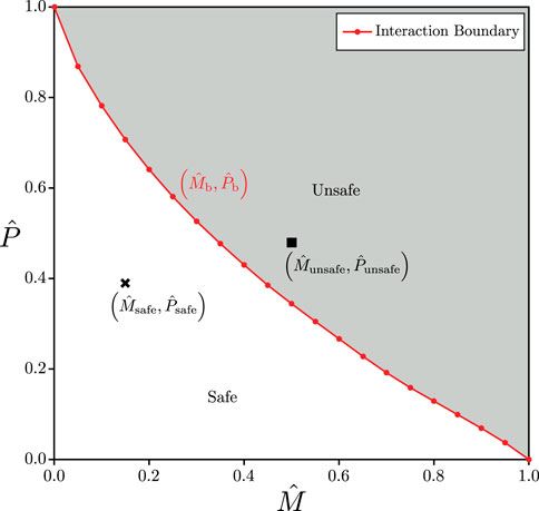
Figure 1. Failure envelope for a beam–column under a combination of normalised uniaxial bending moment
2 Probing SHM methodology for beam–columns
The probing methodology was originally developed by Thompson (2015) to assess the buckling resistance of shells using a non-destructive technique. The process involved loading a cylindrical shell to a prescribed axial compression load and is subsequently probed laterally with a small probing force
The procedure adopted here is similar to that implemented for the study of PSCs (Shen et al., 2023), where the more generic steel beam–column is modelled within the commercial finite element (FE) analysis software application Abaqus (Dassault Systèmes Simulia Corp, 2021). The modelled beam–columns, under a specified combination of axial force
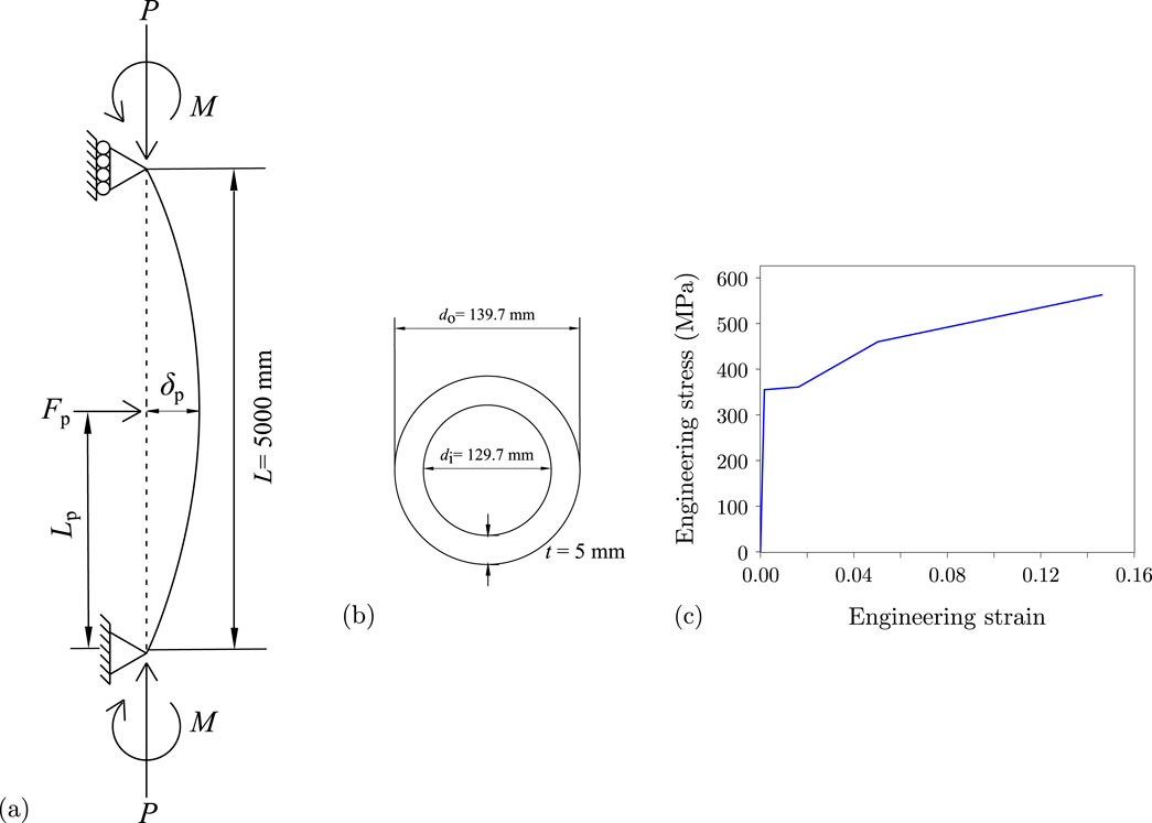
Figure 2. (A) Geometry, loading setup, and boundary conditions of the probing procedure modelled in Abaqus, where the dotted line shows the original state and the solid line depicts the deflected shape during probing; (B) cross section of the beam–column member; (C) engineering stress–strain relationship for the material model used to generate the interaction plot and for the parametric study, as detailed in Table 1.
2.1 FEA model description
An important part of this framework is the FE model of the beam–column. The beam–column considered here is modelled as a simply supported member, as shown in Figure 2. The axial load is applied as a concentrated force at the top of the member, while the uniform uniaxial bending moment is applied as a pair of equal and opposite external moments at its ends, as shown in Figure 2. The geometrical and material properties of the beam–column are given in Table 1.
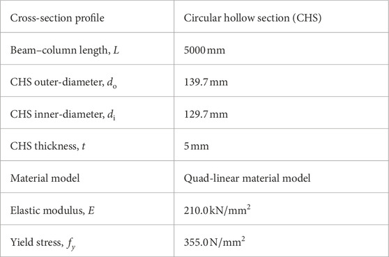
Table 1. Geometrical and material properties used in the parametric study. Note that the “quad-linear material” (QLM) model is defined by Yun and Gardner (2017).
The commercial FE software application Abaqus is used to model the beam–columns, where Timoshenko beam elements with linear interpolation functions (“B21” in the Abaqus element library) are utilised. This choice is appropriate since the interaction between local and global buckling was not within the scope of the current study. Following a mesh sensitivity study, an arrangement comprising 200 beam elements along the main column member is demonstrated to be sufficiently accurate, when verified by comparing the elastic critical buckling load evaluated in FE with the theoretical value from the Euler buckling load
2.2 Beam–column probing parametric study framework
A parametric study was conducted on the presented beam–column by varying the applied moment, applied axial force, and location at which the probe is applied, and the corresponding displacement is measured, as shown in Figure 3. First, a linear buckling analysis (LBA) was executed to obtain the buckling loads and modes of the beam–column. Imperfections were subsequently introduced to the FE model through scaling the first buckling mode by an amplitude of
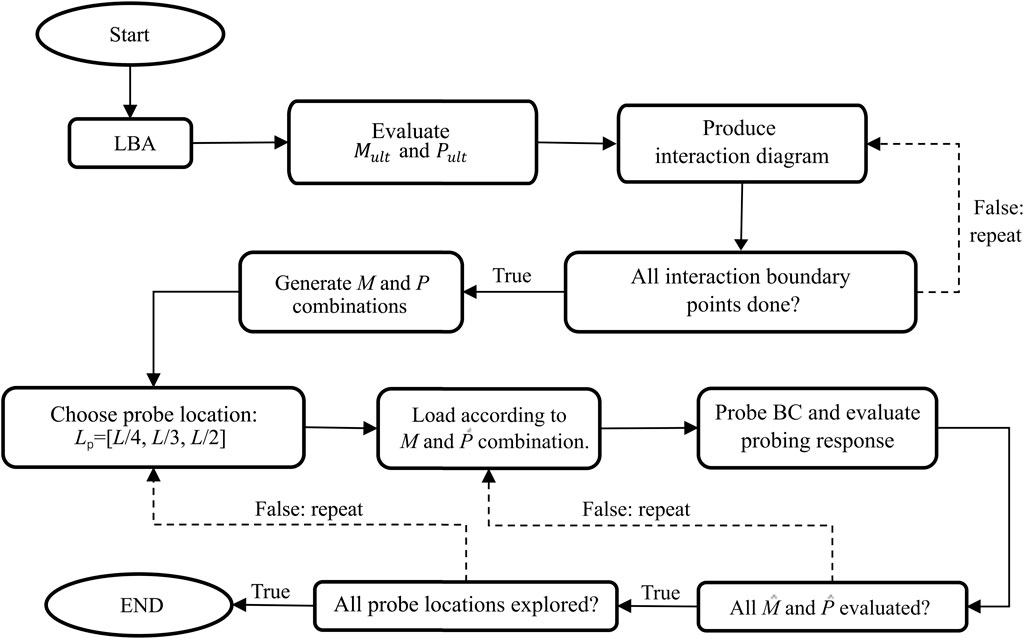
Figure 3. Framework for the parametric study on the probing response of the beam–column.
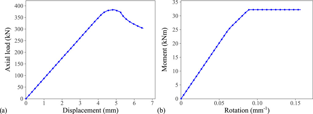
Figure 4. (A) Load–deflection curve of the pure axial case with a peak ultimate load and (B) moment–rotation curve for the pure bending case with no distinct peak.
Having established the values for
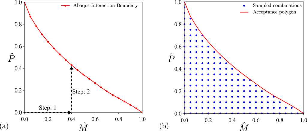
Figure 5. (A) Two-step procedure used to obtain the interaction boundary; (B) combinations of
Finally, the probing study was conducted on the obtained structurally viable combinations of
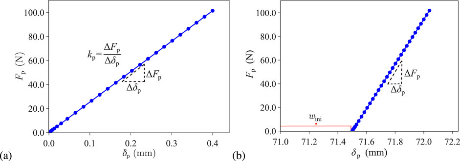
Figure 6. (A) Linear probing response with only
3 Behaviour and probing response of the beam–column
The presence of the in-service bending moment
where
where
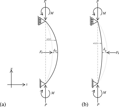
Figure 7. (A) Probing in the direction of deflection (positive direction) exacerbates the deflected shape, leading to a larger curvature, while (B) probing against the direction of deflection (negative direction) leads to a smaller curvature; here,
For a beam–column with uniform bending moment
Thus, by substituting the conditions in Equation 4 into Equation 2, the constants
The deflected profile in Equation 5 is therefore dependent on
Owing to the complex behaviour of beam–columns under combined bending and axial loading, the direction of the probing force
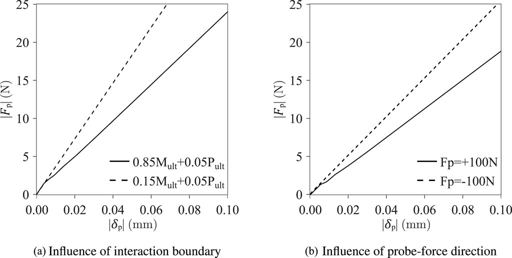
Figure 8. Probing force–displacement response at
A simplified and safe method for identifying the aforementioned “plastic points” is to determine the “elastic boundary” by considering the linear addition of the absolute stress blocks from the applied moment
where
which can be used to eliminate combinations of
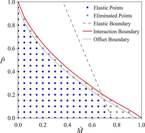
Figure 9. Final combinations of
The probing response for all combinations of
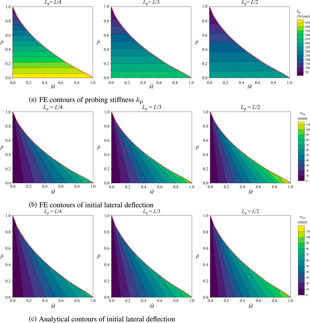
Figure 10. Contours of (A) probing stiffness
Using Equation 5, the FE results can be verified against
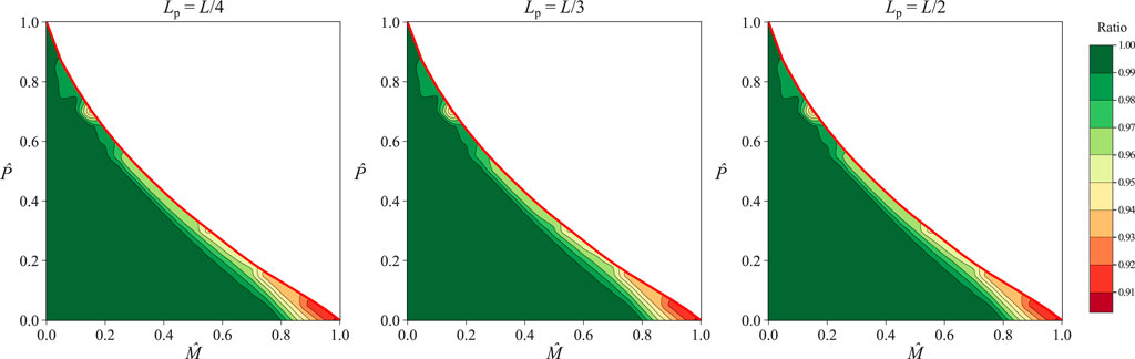
Figure 11. Ratio of analytical to Abaqus
4 Machine learning framework and results
Following the framework developed by Shen et al. (2023), an ANN is implemented for the machine learning framework in the current study to determine whether this can be used to predict
As discussed in Section 3, the probing stiffness response
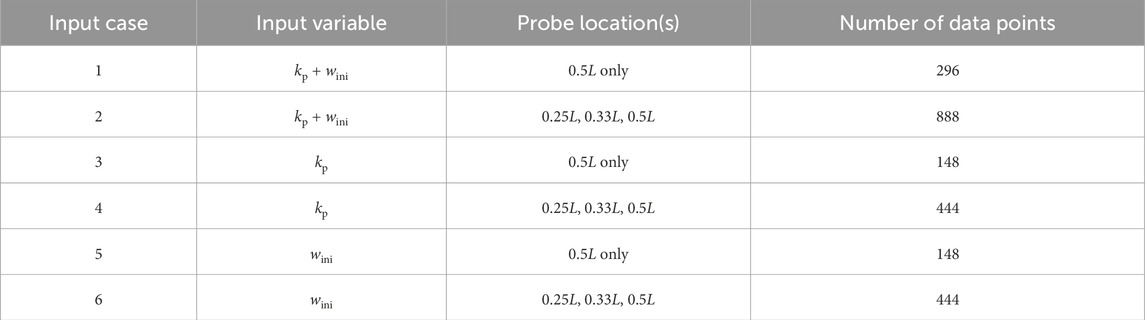
Table 2. Input cases for the ML model and corresponding number of data points.
The ANN model predicts two outputs,
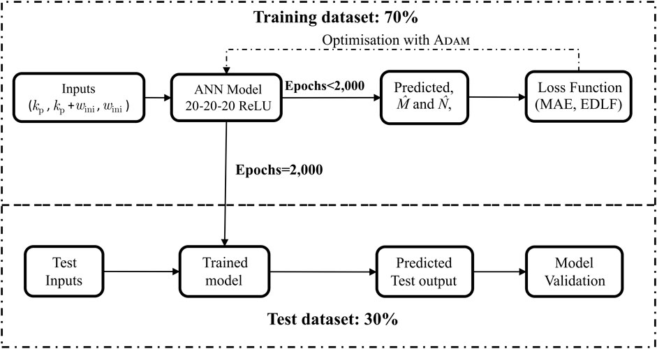
Figure 12. Framework for testing and training the developed ANN.
In the ML framework, loss functions are used to quantify the model error in the training space, and they are used to optimise the weights and bias between each layer in the ANN (Kerkhof et al., 2023). Currently, two types of loss functions are explored, namely, the mean absolute error (MAE) and a bespoke loss function termed “Euclidean distance-loss function” (EDLF) developed by Sung Lee et al. (2020). The difference between the MAE and EDLF is that the MAE computes the average absolute error between the predicted and actual outputs, averaging both the errors of
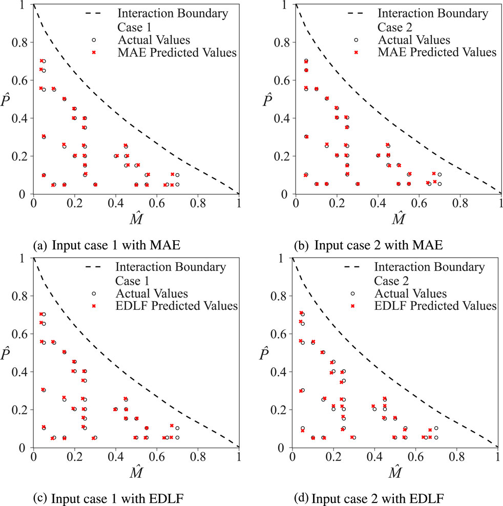
Figure 13. Comparison of the predicted values (ANN results) and the actual values (FE results) on plots of
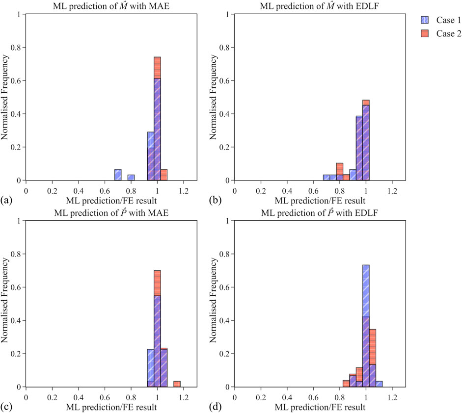
Figure 14. Normalised frequency plots of ML/FE for input cases 1 and 2 with loss functions (A) MAE and (B) EDLF for
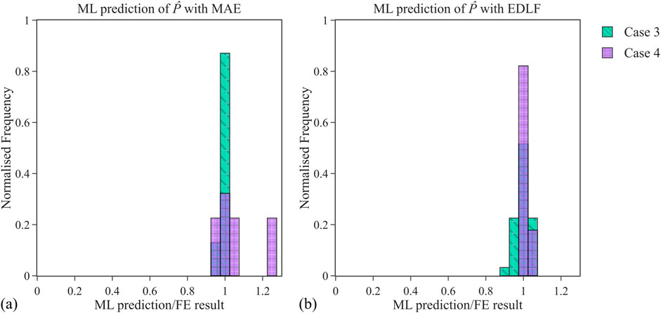
Figure 15. Normalised frequency plots of ML/FE for
4.1 Results
Six input cases and two different loss functions were studied presently, as shown in Table 2. Following the completion of the ANN training procedure presented in Section 4, the evaluation dataset was then used to predict
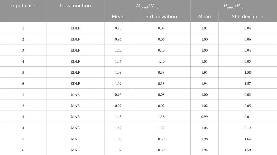
Table 3. Summary of results of
Following the discussion presented in Section 3, it is not surprising that input cases 1 and 2 are determined to be the best performing ANN models, as shown in Table 3, since they utilise data points from both the contours of Figures 10A,B as inputs. Consequently, the model captured the variation in probing responses from both
4.2 Input cases 1 and 2
When comparing the different loss functions for input cases 1 and 2, there is no notable difference in terms of the predicted coordinate and actual coordinate. Both cases predict
Furthermore, the normalised frequency plots shown in Figure 14 suggest that the MAE loss function outperforms EDLF when predicting
4.3 Performance of input cases 3–6
In general, the performance of input cases 3–6 is sub-optimal compared with the results of input cases 1–2, regardless of the loss functions or the number of probe locations considered, as shown in Table 3. Input cases 5–6 are the worst-performing models, regardless of the loss functions used, and are, therefore, not examined further in this study. For input cases 3 and 4, the ML model appears to predict
4.4 Discussion of future developments of the probing ML framework
As noted in Section 3, a key finding from the current work is the recognition that owing to the curvature of the column, which is induced by the applied bending moment, the direction in which the probing force is applied becomes an important parameter in ensuring that the beam–column remains elastic. Therefore, for the probing methodology to be extended to include structural members that also experience bending,
A comprehensive over-fitting study was not performed in the ML model proposed in the current study since the predictions generated by the ML model were sufficiently accurate for input cases 1 and 2, despite the low number of epochs used. Future work can use techniques such as early stopping and
5 Concluding remarks
The probing response of a perfect beam–column that is restrained against the effects of LTB was explored in the current work using the commercial FE software application Abaqus. Owing to a more complex response for probing a beam–column, when compared to a member under pure compression, it is shown that the probing stiffness
The present study also highlights a potential risk associated with the implementation of probing as a structural health assessment tool for beam–columns designed to fail with a plastic ultimate moment of resistance,
Data availability statement
The original contributions presented in the study are included in the article; further inquiries can be directed to the corresponding author.
Author contributions
JM: data curation, formal analysis, investigation, validation, visualization, and writing–original draft. LL: conceptualization, formal analysis, investigation, methodology, project administration, resources, software, supervision, validation, visualization, writing–original draft, and writing–review and editing. MW: conceptualization, methodology, project administration, resources, supervision, and writing–review and editing.
Funding
The author(s) declare that no financial support was received for the research, authorship, and/or publication of this article.
Conflict of interest
The authors declare that the research was conducted in the absence of any commercial or financial relationships that could be construed as a potential conflict of interest.
The author(s) declared that they were an editorial board member of Frontiers, at the time of submission. This had no impact on the peer review process and the final decision.
Publisher’s note
All claims expressed in this article are solely those of the authors and do not necessarily represent those of their affiliated organizations, or those of the publisher, the editors, and the reviewers. Any product that may be evaluated in this article, or claim that may be made by its manufacturer, is not guaranteed or endorsed by the publisher.
References
Abadi, M., Agarwal, A., Barham, P., Brevdo, E., Chen, Z., Citro, C., et al. (2016). Tensorflow: large-scale machine learning on heterogeneous distributed systems. CoRR abs/1603.04467
Alba-Rodríguez, M. D., Martínez-Rocamora, A., González-Vallejo, P., Ferreira-Sánchez, A., and Marrero, M. (2017). Building rehabilitation versus demolition and new construction: economic and environmental assessment. Environ. Impact Assess. Rev. 66, 115–126. doi:10.1016/j.eiar.2017.06.002
Amafabia, D. A., Montalvão, D., David-West, O., and Haritos, G. (2017). A review of structural health monitoring techniques as applied to composite structures. SDHM Struct. Durab. Health Monit. 11, 91–147. doi:10.3970/sdhm.2017.011.091
Arrayago, I., Picci, F., Mirambell, E., and Real, E. (2015). Interaction of bending and axial load for ferritic stainless steel RHS columns. Thin-Walled Struct. 91, 96–107. doi:10.1016/j.tws.2015.02.012
Askar, R., Bragança, L., and Gervásio, H. (2021). Adaptability of buildings: a critical review on the concept evolution. Appl. Sci. Switz. 11, 4483. doi:10.3390/app11104483
Cavajdová, K., and Vican, J. (2023). Resistance of beam-column subjected to compression and bending. Transp. Res. Procedia 74, 983–990. doi:10.1016/j.trpro.2023.11.234
Chen, C. C., Wu, W. H., Liu, C. Y., and Lai, G. (2016). Damage detection of a cable-stayed bridge based on the variation of stay cable forces eliminating environmental temperature effects. Smart Struct. Syst. 17, 859–880. doi:10.12989/SSS.2016.17.6.859
Chollet, F. (2015). Keras. Available at: https://keras.io (Accessed June 3, 2024).
Doebling, S. W., Farrar, C. R., and Prime, M. B. (1998). A summary review of vibration-based damage identification methods. Shock Vib. Dig. 30, 91–105. doi:10.1177/058310249803000201
dos Santos, G. B., Gardner, L., and Kucukler, M. (2018). A method for the numerical derivation of plastic collapse loads. Thin-Walled Struct. 124, 258–277. doi:10.1016/j.tws.2017.11.055
EN (2014). 1993-1-1:2005+A1:2014 Eurocode 3 – design of steel structures – Part 1-1: general rules and rules for buildings. Brussels, Belgium: European Committee for Standardisation CEN.
Fan, W., and Qiao, P. (2011). Vibration-based damage identification methods: a review and comparative study. Struct. Health Monit. 10, 83–111. doi:10.1177/1475921710365419
Favarelli, E., Testi, E., and Giorgetti, A. (2021). Data management in structural health monitoring. Lect. Notes Civ. Eng. 156, 809–823. doi:10.1007/978-3-030-74258-4_51
Gharehbaghi, V. R., Noroozinejad Farsangi, E., Noori, M., Yang, T. Y., Li, S., Nguyen, A., et al. (2022). A critical review on structural health monitoring: definitions, methods and perspectives. Archives Comput. Methods Eng. 29, 2209–2235. doi:10.1007/s11831-021-09665-9
Hakim, S. J., Abdul Razak, H., Ravanfar, S. A., and Mohammadhassani, M. (2014). Structural damage detection using soft computing method. Conf. Proc. Soc. Exp. Mech. Ser. 5, 143–151. doi:10.1007/978-3-319-04570-2_16
Hodson, T. O. (2022). Root-mean-square error (RMSE) or mean absolute error (MAE): when to use them or not. Geosci. Model Dev. 15, 5481–5487. doi:10.5194/gmd-15-5481-2022
Jung, Y., and Hu, J. (2015). A K-fold averaging cross-validation procedure. J. Nonparametric Statistics 27, 167–179. doi:10.1080/10485252.2015.1010532
Katam, R., Pasupuleti, V. D. K., and Kalapatapu, P. (2023). A review on structural health monitoring: past to present. Innov. Infrastruct. Solutions 8, 248–320. doi:10.1007/s41062-023-01217-3
Kerkhof, M., Wu, L., Perin, G., and Picek, S. (2023). No (good) loss no gain: systematic evaluation of loss functions in deep learning-based side-channel analysis. J. Cryptogr. Eng. 13, 311–324. doi:10.1007/s13389-023-00320-6
Kingma, D. P., and Ba, J. L. (2015). “Adam: a method for stochastic optimization,” in 3rd international conference on learning representations, ICLR 2015 - conference track proceedings, 1–15.
Kitipornchai, S., and Trahair, N. S. (1980). Buckling properties of monosymmetric I-beams. ASCE J. Struct. Div. 106, 941–957. doi:10.1061/jsdeag.0005441
Koh, B. H., and Dyke, S. J. (2007). Structural health monitoring for flexible bridge structures using correlation and sensitivity of modal data. Comput. and Struct. 85, 117–130. doi:10.1016/J.COMPSTRUC.2006.09.005
Lapira, L., Wadee, M. A., and Gardner, L. (2017). Stability of multiple-crossarm prestressed stayed columns with additional stay systems. Structures 12, 227–241. doi:10.1016/J.ISTRUC.2017.09.010
Larochelle, H., Bengio, Y., Louradour, J., and Lamblin, P. (2009). Exploring strategies for training deep neural networks. J. Mach. Learn. Res. 10, 1–40. doi:10.5555/1577069.1577070
Liew, A., and Gardner, L. (2015). Ultimate capacity of structural steel cross-sections under compression, bending and combined loading. Structures 1, 2–11. doi:10.1016/j.istruc.2014.07.001
Lindner, J. (1997). Design of steel beams and beam columns. Eng. Struct. 19, 378–384. doi:10.1016/S0141-0296(96)00095-8
Liu, Y., and Nayak, S. (2012). Structural health monitoring: state of the art and perspectives. Jom 64, 789–792. doi:10.1007/s11837-012-0370-9
Martínez, D., Obrien, E. J., and Sevillano, E. (2016). “Damage detection by drive-by monitoring using the vertical displacements of a bridge,” in Insights and innovations in structural engineering, mechanics and computation - proceedings of the 6th international conference on structural engineering (Boca Raton, USA: Mechanics and Computation), 1915–1918. SEMC 2016. doi:10.1201/9781315641645-316
Montavon, G., Orr, G., and Müller, K. (2012). Neural networks: tricks of the trade. 2 edn. Berlin, Heidelberg: Springer. doi:10.1007/978-3-642-35289-8
Publications Office of the European Union (2017). Resource efficient use of mixed wastes improving management of construction and demolition waste: final report. Tech. rep. Publ. Office Eur. Union. doi:10.2779/99903
Riks, E. (1979). An incremental approach to the solution of snapping and buckling problems. Int. J. Solids Struct. 15, 529–551. doi:10.1016/0020-7683(79)90081-7
Ross, B. E., Chen, D. A., Conejos, S., and Khademi, A. (2016). Enabling adaptable buildings: results of a preliminary expert survey. Procedia Eng. 145, 420–427. doi:10.1016/j.proeng.2016.04.009
Rytter, A. (1993). Vibration based inspection of civil engineering structures. Denmark: Aalborg University. Ph.D. thesis.
Saito, D., and Wadee, M. A. (2008). Post-buckling behaviour of prestressed steel stayed columns. Eng. Struct. 30, 1224–1239. doi:10.1016/J.ENGSTRUCT.2007.07.012
Shen, J., Lapira, L., Wadee, M. A., Gardner, L., Pirrera, A., and Groh, R. M. (2023). Probing in situ capacities of prestressed stayed columns: towards a novel structural health monitoring technique. Philosophical Trans. R. Soc. A Math. Phys. Eng. Sci. 381, 20220033. doi:10.1098/rsta.2022.0033
Shokravi, H., Shokravi, H., Bakhary, N., Rahimian Koloor, S. S., and Petrů, M. (2020). Health monitoring of civil infrastructures by subspace system identification method: an overview. Appl. Sci. Switz. 10, 2786. doi:10.3390/APP10082786
Slaughter, E. S. (2001). Design strategies to increase building flexibility. Build. Res. Inf. 29, 208–217. doi:10.1080/09613210010027693
Sumitro, S., and Wang, M. L. (2005). Sustainable structural health monitoring system. Struct. Control Health Monit. 12, 445–467. doi:10.1002/STC.79
Sung Lee, B., Phattharaphon, R., Yean, S., Liu, J., and Shakya, M. (2020). “Euclidean distance based loss function for eye-gaze estimation,” in IEEE Sensors Applications Symposium, SAS 2020 - Proceedings, Kuala Lumpur, Malaysia, 09-11 March 2020, 1–5. doi:10.1109/SAS48726.2020.9220051
Tao, F., Liu, X., Du, H., and Yu, W. (2020). Physics-informed artificial neural network approach for axial compression buckling analysis of thin-walled cylinder. AIAA Scitech 2020 Forum 1 PartF, 1–18. doi:10.2514/6.2020-0398
Thompson, J. M. T. (2015). Advances in shell buckling: theory and experiments. Int. J. Bifurcation Chaos 25, 1530001–1530025. doi:10.1142/S0218127415300013
Thomson, D. J. (2013). The economic case for service life extension of structures using structural health monitoring based on the delayed cost of borrowing. J. Civ. Struct. Health Monit. 3, 335–340. doi:10.1007/s13349-013-0057-0
Trahair, N. S., Bradford, M. A., Nethercot, D. A., and Gardner, L. (2008). The behaviour and design of steel structures to EC3. Abingdon, UK: CRC Press.
UNEP (2020). Towards a zero-emissions, efficient and resilient buildings and construction sector. Glob. Status Rep. Build. Constr. 2020, 9–10.
Wu, B., Wu, G., Yang, C., and He, Y. (2018). Damage identification method for continuous girder bridges based on spatially-distributed long-gauge strain sensing under moving loads. Mech. Syst. Signal Process. 104, 415–435. doi:10.1016/J.YMSSP.2017.10.040
Wu, K., Qiang, X., Xing, Z., and Jiang, X. (2022). Buckling in prestressed stayed beam–columns and intelligent evaluation. Eng. Struct. 255, 113902. doi:10.1016/j.engstruct.2022.113902
Xing, Z., Wu, K., Su, A., Wang, Y., and Zhou, G. (2023). Intelligent local buckling design of stainless steel I-sections in fire via Artificial Neural Network. Structures 58, 105356. doi:10.1016/j.istruc.2023.105356
Keywords: beam–columns, structural stability, on-site assessment, structural health monitoring, machine learning
Citation: Ma JT, Lapira L and Wadee MA (2024) Enhancing the assessment of in situ beam–column strength through probing and machine learning. Front. Built Environ. 10:1492235. doi: 10.3389/fbuil.2024.1492235
Received: 06 September 2024; Accepted: 18 November 2024;
Published: 11 December 2024.
Edited by:
Jing-Zhong Tong, Zhejiang University, ChinaCopyright © 2024 Ma, Lapira and Wadee. This is an open-access article distributed under the terms of the Creative Commons Attribution License (CC BY). The use, distribution or reproduction in other forums is permitted, provided the original author(s) and the copyright owner(s) are credited and that the original publication in this journal is cited, in accordance with accepted academic practice. No use, distribution or reproduction is permitted which does not comply with these terms.
*Correspondence: Luke Lapira, bC5sYXBpcmFAdWNsLmFjLnVr