 Syed Md Yousuf1Mehboob Anwer Khan1Syed Muhammad Ibrahim1
 Furquan Ahmad2*
 Pijush Samui2Anil Kumar Sharma2
- 1Department of Civil Engineering, ZHCET, AMU, Aligarh, India
- 2Department of Civil Engineering, National Institute of Technology, Patna, Bihar, India
Improving soil strength and reducing the anticipated settlement and construction cost is a great paradox for civil as well as geotechnical engineers. In this paper, these aspects and other suitable types of ground improvement are discussed based on the principles of using geosynthetics for soil reinforcement. A series of load-settlement tests were also performed to compare strength and settlement of the silty sand reinforced with lime and one layer of geotextile. The study finds the maximum insertions of geotextile at 0.2D (3.0 cm) beneath the square footing base, and the lime percentage of 5.0% increases the UBC substantially. The UBC of lime-treated and geotextile-reinforced silty sand was to an optimum of 1,360 kN/m2 that has shown an enhancement of 258% compared to that of untreated and unreinforced silty sand that is approximately 380 kN/m2. Furthermore, comparative analysis between two ANN models was performed to provide improved estimate of the UBC, namely artificial neural network (ANN) and extreme learning machine (ELM). The developed computational models were then compared with experiment data, which proved that such models are more economical and effective than the expensive and time consuming conventional techniques. Consequently, based on the results, it was further validated that ELM possesses better generalization capability compared to ANN for predictive efficiency and thereby proves the efficiency of the model in estimating the ultimate bearing capacity of square footings incorporated with geotextile and lime-treated silty sand. This places the ELM model as a useful tool in the initial conceptual as well as the design for improvement steps of soil reinforcement.
1 Introduction
Enhancing soil characteristics in construction endeavours remains an ongoing challenge. Ground improvement holds a crucial position in civil construction, and various innovative technologies and approaches have been devised to assist geotechnical engineers in delivering cost-effective solutions for construction on complex sites (Yousuf et al., 2024; Yousuf et al., 2023; Zhang C. et al., 2022; Huang et al., 2023; Huang et al., 2022; Xu et al., 2022; Yu et al., 2021).
The idea of reinforcing with fibres has a history spanning over 5,000 years, as early civilizations utilized materials such as straw and hay to bolster the stability of mud blocks (Abtahi et al., 2009). Ancient Chinese, Romans, and Incas implemented diverse techniques to improve soil strength, and some of these methods have endured through the ages. In India, the contemporary era of soil stabilization commenced in the early 1970s, although antiquated approaches resulted in a diminishing regard for soil stabilization practices. The process of soil stabilization entails altering the geotechnical properties of soil to align with engineering specifications. Soils are generally categorized into gravel, sand, silt, and clay, with some containing high amounts of montmorillonite, leading to swelling and shrinkage with water (Steinberg, 2000).
Subgrade preparation for pavement construction can be time-consuming, especially when dealing with soft subgrade conditions. Traditional methods, such as recompacting the subgrade or undercutting and replacement, are labour-intensive and costly. Alternative methods involve treating weak soil with lime or reinforcing it with geosynthetics like geotextiles or geogrids. Lime-soil treatment involves a chemical process in which lime reacts with clay particles within the soil, forming a cementitious matrix. Geosynthetics reinforce the soil mechanically through separation, confinement, and/or reinforcement. Recently, soil stabilization has gained renewed attention due to increased demand for economic development, basic materials, and fuel. Advanced research, building materials, and equipment have made soil stabilization a recognized and cost-effective method for soil improvement (Malhotra and John, 1986).
Studies have shown the effectiveness of adding brick pieces to fly ash-lime stabilized expansive soil, resulting in improved strength and durability at a lower cost than conventional materials (Malhotra and John, 1986). Geosynthetics, such as geofabrics, geotextiles, geomembranes, and geogrids, constructed from polymers like polyester and polypropylene, are engineered to improve geotechnical and engineering characteristics. Geosynthetics can serve various functions, including separation, reinforcement, drainage, and containment (Das and Khing, 1994). In pavement design, the widespread utilization of geotextiles and geogrids aims to enhance performance, decrease thickness, and prolong the service life (Cancelli et al., 1992; Guram et al., 1994). Geogrids of high stiffness have shown better performance, and their use has been associated with improved pavement thickness reduction (Miura et al., 1990).
The adoption of artificial intelligence (AI) techniques, such as artificial neural networks (ANN), for predicting parameters in pavement design has gained prominence in recent decades. AI has been applied to identify and analyse pavement surface cracks, predict the resilient modulus of subgrade soil, and assess subgrade soil stabilization (Kaseko and Ritchie, 1993; Sadrossadat et al., 2016; Zaman et al., 2010). AI methods, including ANN, have also been utilized to anticipate the settlement and load-bearing capacity of piles in foundation engineering issues (Rahman et al., 2001; Liu et al., 2020). In the present study, the author employs two computational approaches, ANN and extreme learning machine (ELM), to validate experimental data (ultimate bearing capacity) with multiple input variables. The objectives of this investigation include:
1. Determine the ultimate bearing capacity (UBC) solely for the untreated silty-sand soil.
2. Evaluate UBC of soil with varying percentages (%) of lime only.
3. Assess the ultimate bearing capacity of the soil with a single layer of geotextile at different depths exclusively.
4. Determine the UBC of the soil under the combined influence of geotextile and lime.
5. Examine the ideal lime percentage and the optimal depth of geotextile to achieve the ultimate bearing capacity (UBC) for square footing.
6. Verify the experimental results of ultimate bearing capacity (UBC) using computational models, such as ANN and ELM.
2 Methodology
This section provides a detailed account of the materials utilized in the study, including silty-sand, lime, and geotextile, along with their compositions and geotechnical properties. Furthermore, the section provides clarity on the experimental procedures, outlining the creation of computational models like ANN and ELM, along with the crucial statistical performance metrics utilized to evaluate the efficiency of these models. Notably, the study concurrently conducted both computational methods and experimental investigations. In essence, the validation of test results was conducted using computational models to anticipate the ultimate bearing capacity of soils.
2.1 Experimental approach
2.1.1 Materials
Silty sand, sourced from Narora Barrage in Uttar Pradesh, India, adjacent to the Ganges River, is acknowledged as a residual material. Employing this silty sand not only provides a cost-effective option for civil engineering construction but also addresses environmental concerns such as leaching, waterway obstruction, and negative impacts on aquatic life. The aim is to derive value from the waste. Figure 1 illustrates the particle size distribution curve of the silty sand.
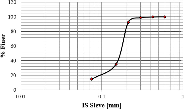
Figure 1. Representation of particle size distribution curve of silty sand.
During the laboratory tests, the silty sand consistently maintained a dry state and exhibited a fineness finer than the 4.75 mm sieve. Table 1 provides the geotechnical properties of the silty sand. In this study, a polypropylene nonwoven geotextile supplied by the Central Soil and Materials Research Station in Delhi was employed. Table 2 outlines the geotechnical properties of the geotextile, and Figure 2 provides a visual representation of the geotextile.
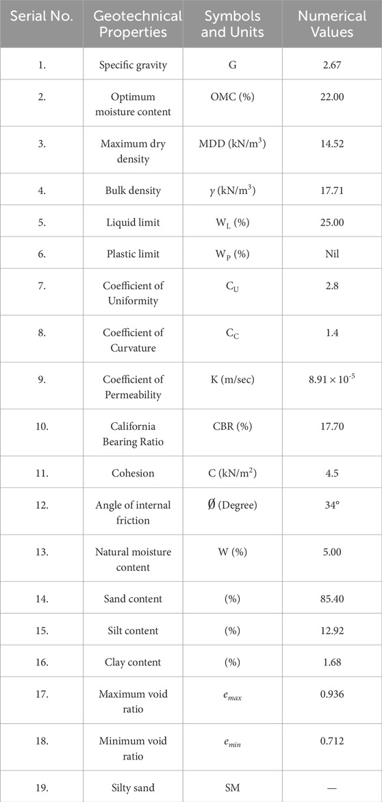
Table 1. Characteristics of silty sand from a geotechnical perspective.
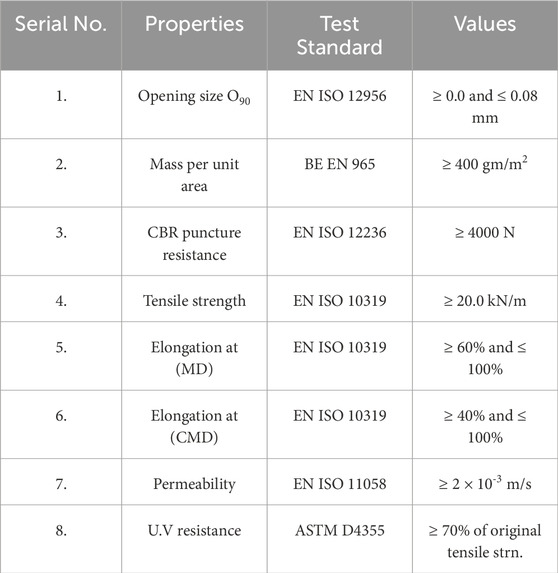
Table 2. Geotextile properties.
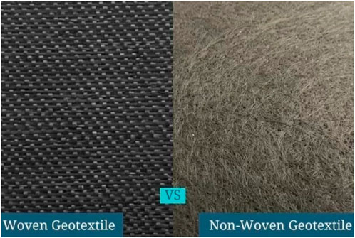
Figure 2. Image of woven and nonwoven geotextile (source: geosyntheticmagazine.com).
The use of lime for stabilisation is a historical and essential strategy for ground improvement, with major efforts dating back to 1925 (Pal and Ghosh, 2014). Lime is produced by heating limestone (CaCO3) to a high temperature of 1,100°C. Quicklime (CaO) reacts with water to generate hydrated lime (Ca(OH)2). The interaction of hydrated lime with soil particles causes a pozzolanic reaction, which results in the production of a strong cementitious matrix (Ali and Korranne, 2011). The chemical reaction between quicklime and water is described below, in Equation 1.
This is an exothermic reaction, and the pH value increases to approximately 12.5. This scenario is conducive to initiating the pozzolanic reaction Bose (Bose, 2012). Tables 3, 4 show the chemical compositions of additive quick lime and silty sand, respectively.

Table 3. Admixture quick lime Chemical composition.
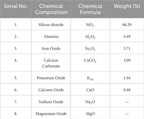
Table 4. Silty sand chemical composition.
In this study, the quicklime needed for the project was obtained at a local market in Jamalpur, near the A.M.U. campus. Tables 3, 4 provide details on the chemical compositions of the admixture, quicklime, and soil. The appearance and chemical content of lime and silty sand were examined using optical microscopy at Aligarh Muslim University’s Sophisticated Instruments Facility (USIF) in the Central Instrumentation Facility Laboratory. Figures 3, 4 show the SEM and Energy-dispersive X-ray spectroscopy (EDS) examinations of lime and silty sand, respectively.
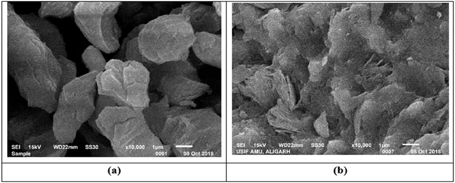
Figure 3. Scanning of electron microscope (SEM) at
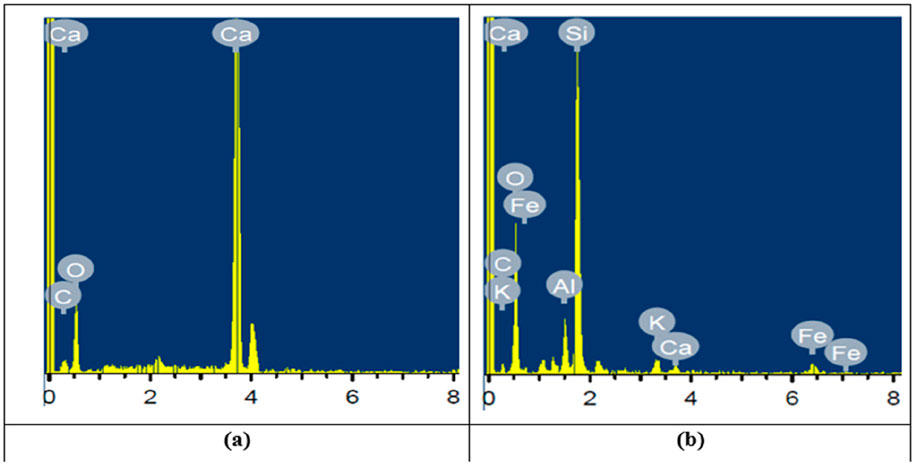
Figure 4. EDS of (A) Lime (B) Silty sand.
2.1.2 Experimental approach
In this study, the soil samples underwent treatment with varying proportions of lime, ranging from 0% to 6%, with a minor increment of 0.5%. Concurrently, geotextile reinforcement was applied to the soil at specific depths (0.2D, 0.4D, 0.6D, 0.8D, 1.0D, 1.2D) for each lime percentage, and the investigation focused on the UBC and the corresponding soil deflection. A grand total of 91 experiments were conducted, comprising scenarios both with and without the use of geotextile. The experiments utilized square footings with a surface area of 100 cm2, each measuring 10 cm × 10 cm. The variable ‘D' represents the maximum depth of the pressure bulb formed beneath the footing pedestal. In the case of the square footing, D is equivalent to 1.5 times the length of the side (10 cm), which totals 15 cm. Concerning square footing, the specific measurements for 0.2D, 0.4D, 0.6D, 0.8D, 1.0D, and 1.2D are as follows: 3.0 cm, 6.0 cm, 9.0 cm, 12.0 cm, 15.0 cm, and 18.0 cm, respectively. The detailed overview of the experimental program is outlined in Table 5.
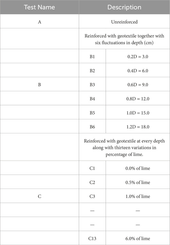
Table 5. Experimental program details.
2.1.3 Setup for experimental trials
The tank utilized in the experiment had dimensions of 50 cm in length, 50 cm in width, and 75 cm in height. This configuration was selected to consider the overlapping pressure zone of the footing and the potential impact of the tank walls on the pressure zone. After achieving the required density, a single layer of geotextile was placed at various depths, as mentioned earlier. The square footing was positioned at the center of the tank’s top surface. The entire system was then loaded with a point load applied axially through a ball positioned in a groove at the center of the footing. The least counts on the load and settlement dial gauges were 7.5 N/div and 0.01 mm/div, respectively. Figure 5 illustrates the experimental load tank along with the load and settlement dial gauges.
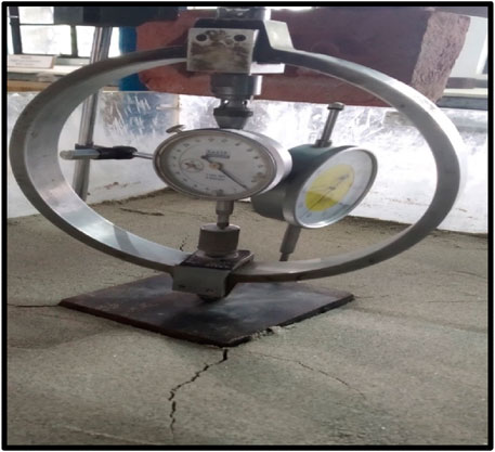
Figure 5. Experimental arrangement featuring load and settlement dial gauges.
A graph was generated with “Load” plotted on the X-axis and ‘Settlement’ on the Y-axis to determine the ultimate bearing capacity (UBC) and the associated settlement. Subsequently, a graph was produced, and the UBC along with their corresponding settlement were computed utilizing the “double tangent method,” as depicted in Figure 6 below.
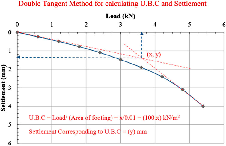
Figure 6. Load-Settlement Curve in the laboratory model plate-load test for determining Ultimate Bearing Capacity (UBC) and settlement, utilizing the Double Tangent Method for calculation.
2.2 Computational method
2.2.1 Statistical performance metrics
A comprehensive set of commonly employed statistical metrics was utilized to evaluate the effectiveness of the predictive models. These metrics include the correlation coefficient (R), coefficient of determination (R2), adjusted determination coefficient (Adj.R2), weighted mean absolute percentage error (WMAPE), Nash-Sutcliffe efficiency coefficient (NS), variance account factor (VAF), root mean square error (RMSE), reduced simple ratio (RSR), Willmott’s Index (WI), Normalized mean bias error (NMBE), mean absolute percentage error (MAPE), Legate and McCabe’s Index (LMI), Bias Factor (BF), Mean absolute error (MAE), Mean bias error (MBA) and A20-index (Ghani et al., 2021; Ghani and Kumari, 2021a; Ghani and Kumari, 2021b).
The parameters R, R2, and Adj.R2 are employed to assess the model’s performance in the soil, with the ideal value for these parameters being 1. The Bias Factor (BF) serves as a constant, allowing flexibility for optimal performance, and its ideal value is 1. NS reflects the model’s forecasting capability, and its optimal value is 1. Willmott’s Index (WI) serves as an indicator of the error in predicting the targeted value, with its optimal value established at 1. The Variance Account Factor (VAF) value delineates performance, and the ideal value for optimal performance is 100. Weighted Mean Absolute Percentage Error (WMAPE) represents the degree of accuracy in prediction, and a value closer to zero signifies better accuracy. Reduced Simple Ratio (RSR) is a parameter reflecting the precision in prediction, and its optimal value is zero. MAPE showcases accuracy in forecasting, with a value closer to zero indicating better accuracy. NMBE demonstrates the percentage of bias in predicted values from the mean, and its optimal value is zero. The A20-index assesses the number of samples that align with prediction values within a deviation of ±20% compared to experimental values, with an ideal value set at 1. Numerous researchers have adopted these statistical values to examine the accuracy and precision of computational models. The tabulated information for the statistical performance metrices mentioned earlier is presented in Table 6.
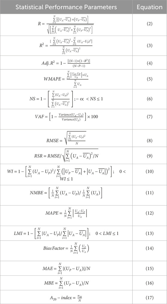
Table 6. Statistical performance metrics equations.
In the given context,
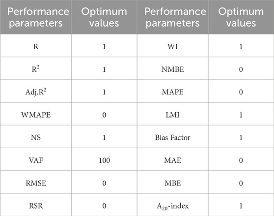
Table 7. Ideal values of the statistical performance metrics.
Utilizing these metrices facilitates an easy assessment of the precision in compiling experimental data and selecting the most effective forecasting model. Elevated values of R, R2, Adj. R2, NS, WI, LMI, Bias Factor, A20-index, and VAF signify a higher value for the developed model. On the other hand, decreased values of RMSE, WMAPE, RSR, MAE, MBE, NMBE, and MAPE indicate an enhanced forecasting ability of the model. The following section offers an in-depth estimation and illustration of these performance parameters.
2.2.2 Taylor’s diagram
A graphical representation known as a “Taylor’s diagram” is employed to visually depict and compare the performance of the established computational models. This diagram was designed to demonstrate the accuracy of several artificial intelligence systems in a concise and simply understandable manner Ghani et al. (2021). With a singular point on the diagram, it displays statistical performance indicators such as the Pearson correlation coefficient, RMSE, and standard deviations between the two variations. The point closest to the “reference point” on the diagram represents the best effective forecasting model. This study generates Taylor’s diagrams for the developed computational models, which include ANN and ELM, while taking into account both training and testing datasets.
2.2.3 Artificial neural network (ANN)
ANN is a crucial component of expert systems designed to emulate human cognitive processes. An ANN model can analyze and comprehend given information, efficiently tackling complex problems that may prove challenging for human or traditional mathematical approaches. With automatic learning capabilities, ANNs can produce superior outcomes.
An artificial neural network has three main components: neurons, network design, and a learning rule. Figure 7 depicts the standard construction of a model ANN. A lower number of hidden neurons may result in major training errors, whereas a higher number of hidden neurons may result in minor training errors but significant testing errors due to increased variability.
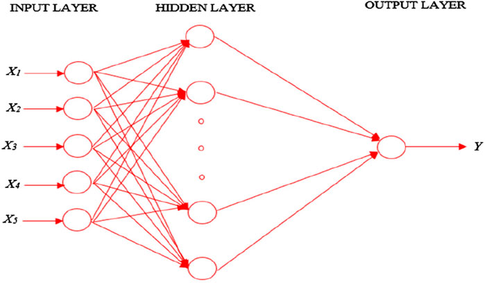
Figure 7. A typical architecture of ANN.
Artificial Neural Networks (ANNs), akin to human cognitive processes, utilize rules and laws, referred to as backpropagation, to generate outcomes. During the training phase, ANNs recognize patterns and trends in data, whether visual, auditory, or textual. The system’s network compares predicted values with actual values, and the difference is adjusted using backpropagation. To minimize the disparity between actual and predicted values, the system functions in reverse, moving from the output to the input units.
The field of artificial neural networks was initiated by Warren McCulloch and Walter Pitts (McCulloch and Walter, 1943) and subsequent developments include the invention of calculators by Farley and Clark, (1954) the derivation of continuous backpropagation basics by Kelley and Bryson (Kelley, 1960; Bryson, 1961) and Rumelhart, Hinton, and Williams (David et al., 1986) demonstrating backpropagation’s ability to learn representations of words. Advancements in the field have continued, with applications ranging from recognizing higher-level concepts to evaluating risks in geotechnical engineering.
In recent years, ANNs have found success in various engineering fields, particularly in geotechnical engineering. They have been effective in predicting pile load capacity, modeling soil behavior, site description, earth retaining construction, slope stability, tunnel design, soil liquefaction, porosity, soil contraction, soil expansion, and soil classification. However, today’s expert systems, like as ANN, employed to mimic the human brain are analogous to comparing a paper plane to a supersonic jet. Mughieda et al. (2009).
A dedicated ANN model has been formulated to predict the ultimate bearing capacity (UBC) of a square footing, considering parameters such as length, breadth, footing area, depth of geotextile, lime percentage, maximum load, maximum settlement, and settlement corresponding to UBC. The model utilizes a single hidden layer with 14 neurons and undergoes extensive training through multiple iterations and confirmation checks. The MATLAB code for the ANN is provided in Annexure-1.
2.2.4 Extreme learning machine
ELM technology has recently gained widespread acceptance among scholars. It proves to be a valuable and resilient method for establishing connections between input index parameters and their corresponding output variables. ELM, devised by Guang-Bin Huang (Huang et al., 2006) represents an adapted version of the conventional ANN model. Huang claimed that the ELM model is capable of outperforming networks trained via backpropagation, such as ANN, in terms of conceptual performance, accuracy, and speed. ELM stands out as an innovative machine learning model that randomly selects hidden nodes and systematically calculates weights within a single-layer feedforward network (Huang et al., 2006; Huang et al., 2011). The ELM model program was developed using MATLAB, and Figure 8 illustrates the fundamental operational principle of the ELM model.
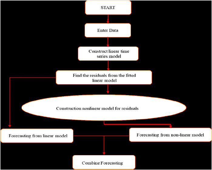
Figure 8. Flowchart of (ELM) model.
The ELM model proved useful in a variety of applications, including classification, soil liquefaction susceptibility, regression analysis, bearing capacity prediction. In summary, due to its swift and systematic learning speed, rapid convergence, improved generalization capacity, user-friendly application, and high accuracy, the ELM model offers substantial advantages in generating correlations between input and output variables Chen et al. (2017).
A single hidden layer ELM model, incorporating 14 neurons and leveraging various parameters, has been developed to predict the ultimate bearing capacity of a square foundation. The model considers input factors such as length, breadth, footing area, geotextile position from the bottom of the footing, percentage of lime, maximum load, maximum settlement, and settlement corresponding to ultimate bearing capacity. The MATLAB code for the ELM is provided in Annexure-2.
3 Result and discussions
This section is divided into two parts. Firstly, the outcomes of adjusting the geotextile position (0.2D, 0.4D, 0.6D, 0.8D, 1.0D, 1.2D, and without geotextile) are presented to determine the “optimal depth.” Secondly, the results derived from varying the percentage (0%, 0.5%, 1.0%, 1.5%, ------, up to 6.0%) of lime at the optimal geotextile depth are depicted and elucidated in the subsequent section, aiming to establish the “optimal (%) of lime”. As a result, the total number of tests completed, considering the optimum depth, with and without geotextile, is 7 + 13 = 20.
The validity of the results will be computationally tested in the following part using ANN and ELM. The author applied varying percentages of lime at each level of the geotextile to match the data requirements for these computer analyses. As a result, the total number of tests performed, with and without geotextile, is 7 × 13 = 91. Table 8 summarizes the findings of these ninety-one tests.
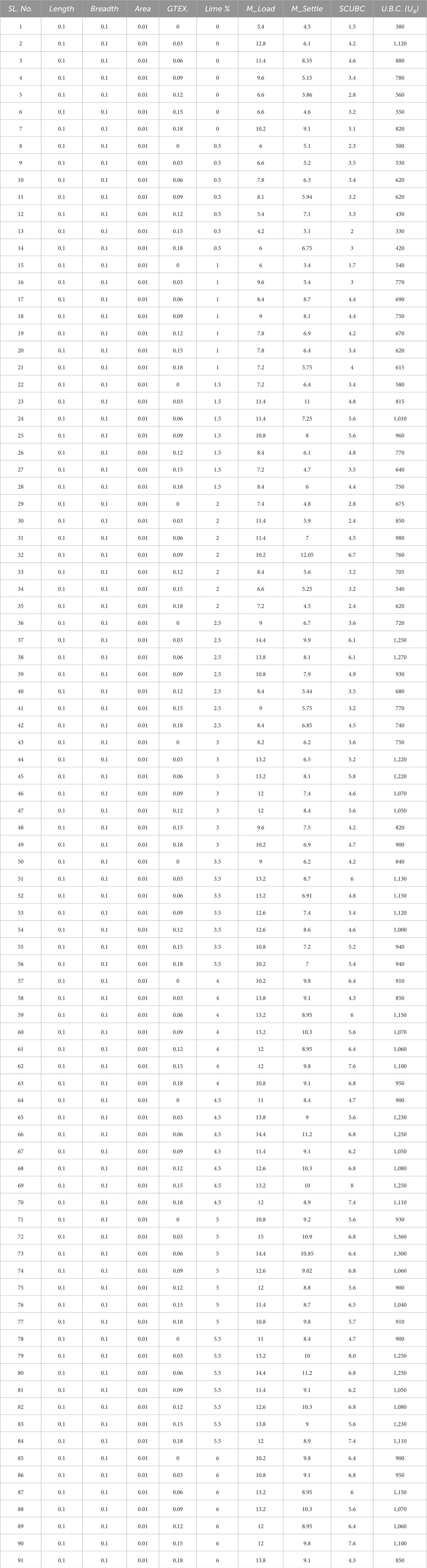
Table 8. Experimental test data.
3.1 Outcomes of UBC of square footing for calculating optimum depth of geotextile
3.1.1 Experimental method
Figure 9 illustrates the correlation between load and settlement for silty sand with geotextile positioned at different depths from the base of the footing: 0.2D, 0.4D, 0.6D, 0.8D, 1.0D, and 1.2D. The study reveals that the maximum failure stress of the soil occurs when the geotextile is situated at a depth of 0.2D, or 3.0 cm from the base of the square footing. The ultimate bearing capabilities (kN/m2) of the soil were calculated using the double tangent method at various geotextile depths. The results show that the ultimate bearing capacities were 380, 1,120, 880, 780, 560, 550, and 820 kN/m2, when a single layer of geotextile is placed at different depths such as: without geotextile, 0.2D, 0.4D, 0.6D, 0.8D, 1.0D, and 1.2D, respectively. As a result, the ideal geotextile depth was determined to be 0.2D (3.0 cm) from the square footing’s base.
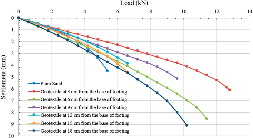
Figure 9. Load v/s settlement graph for reinforced as well as unreinforced soil sample without lime, while one layer of geotextile is at varying depths from the base of the footing. (Experimental Test Data).
Figure 10 depicts the load versus settlement curve for a geotextile positioned at a depth of 0.2D (3.0 cm) from the footing’s base. The UBC is determined using the double tangent method to be 1,120 kN/m2.
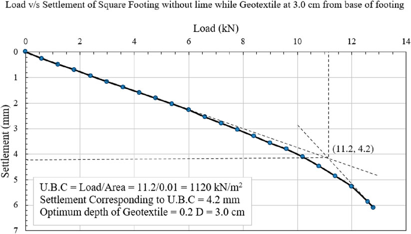
Figure 10. Load v/s settlement graph when geotextile is at 3.0 cm from the base of the footing.
3.2 Results for the ultimate bearing capacity of square footing to determine the optimal percentage (%) of lime
3.2.1 Experimental method
By securing the geotextile at the optimal depth, the investigation of lime % variation was expanded. Concurrently, the geotextile was positioned at a depth of 3.0 cm from the base of the square footing, and the lime percentage was adjusted from 0.0% to 0.5%, 1.0%, 1.5%, ------, up to 6.0%. Under these conditions, Figure 11 depicts the load versus settlement plot of silty sand. The figure illustrates that soil treated with 5.0% lime exhibits the maximum failure load (UBC). The ultimate bearing capacity (UBC) of the soil (in kN/m2) was determined using the double tangent method with a single layer of geotextile positioned at a depth of 0.2D (3.0 cm) from the base of the square footing, while varying the lime percentage from 0.0%, 0.5%, 1.0%, 1.5%, 2.0%, 2.5%, 3.0%, 3.5%, 4.0%, 4.5%, 5.0%, 5.5% and 6.0%. The UBC values for various lime percentages were 1,120, 530, 770, 815, 850, 1,250, 1,220, 1,130, 850, 1,230, 1,360, 1,250, and 950 kN/m2, according to the results. In simpler terms, the optimal depth and optimal lime percentage for a square footing are 0.2D (3.0 cm) and 5.0% of the dry weight of silty sand, respectively. The equivalent UBC optimal value is 1,360 kN/m2.
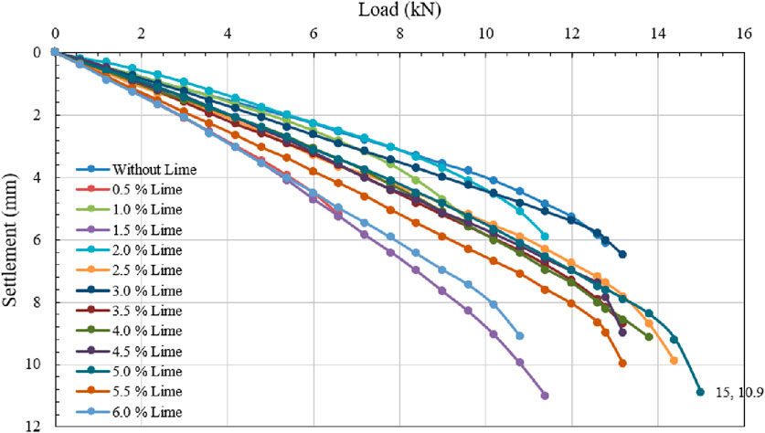
Figure 11. Load versus settlement graph for changing % of lime when geotextile is placed at a fixed optimum depth of 0.2D = 3.0 cm from the bottom of a square footing. (Experimental test data).
Figure 12 illustrates the load versus settlement graph for the condition where the geotextile is placed at a depth of 0.2D (3 cm) from the base of the square footing, and the lime percentage is fixed at 5.0%. The calculated ultimate bearing capacity using the double tangent approach is 1,360 kN/m2.

Figure 12. Load v/s settlement graph, lime is 5.0% and geotextile is placed at 3.0 cm from the base of the footing.
4 Evaluation of performance using computational models such as ANN and ELM
4.1 Experimental method adopted for square footing reinforced by geotextile
Laboratory experiments were conducted for a square footing on silty sand, incorporating geotextile reinforcement and lime treatment. The test data, encompassing parameters such as footing size, footing area, geotextile depth, lime percentage, maximum load at failure, maximum settlement at failure, settlement at ultimate bearing capacity, and ultimate bearing capacity, is presented in Table 8. This comprehensive experimental dataset will be further analyzed using two artificial intelligence methods: ANN and ELM repectively.
In this situation, there are eight independent variables: length of square footing (m), breadth of square footing (m), area of the footing (m2), depth of geotextile from the base of the footing “GTEX” (m), percentage (%) of lime, maximum load “M_Load” (kN), maximum settlement “M_Settle” (mm), settlement corresponding to ultimate bearing capacity “SCUBC” (mm), and one dependent variable named experimental ultimate bearing capacity. To assess validity, 68 (75%) of the total 91 test data points were chosen at random for the training dataset, while the remaining 23 (25%) comprise the testing dataset, as shown in Tables 9, 10 respectively. Both ANN and ELM estimated ultimate bearing capacity (kN/m2) is marked by “UP”.
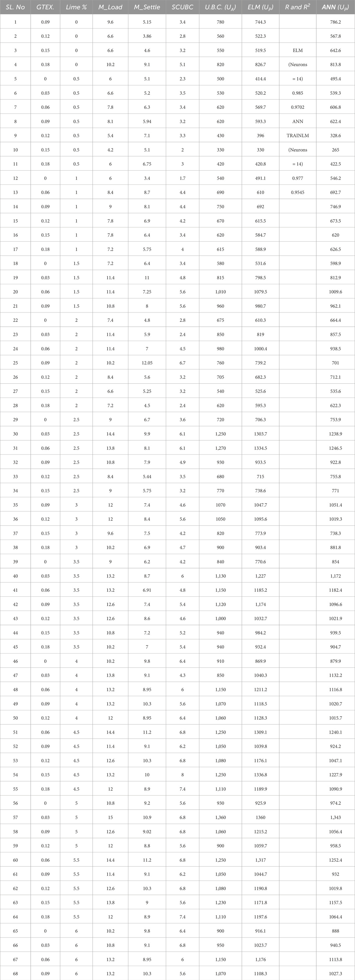
Table 9. Training data.
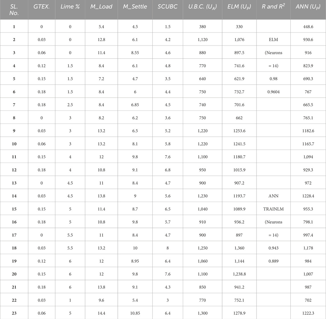
Table 10. Testing data.
4.2 Computational method for square footing reinforced by geotextile
This section details the application of the developed computer models to predict the ultimate bearing capacity. Utilizing input parameters such as length, breadth, area, geotextile depth (GTEX), lime percentage, maximum load, maximum settlement, and settlement corresponding to ultimate bearing capacity (SCUBC). Two robust computational methodologies, namely ANN and ELM, were used to predict the UBC. The generated models exhibit commendable prediction accuracy, as depicted in Figure 13, illustrating a 2-dimensional scatter plot of the key input factors and the target output variable, UBC.
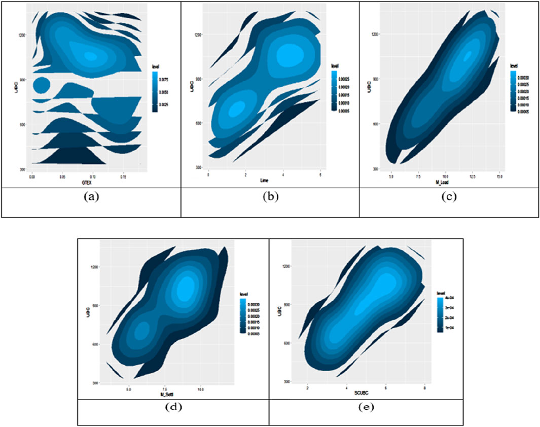
Figure 13. 2-D scatter plot of independent variable (A) GTEX (B) lime percentage (C) max_load (D) max_settlement (E) SCUBC.
Figure 14 illustrates the prediction of ultimate bearing capacity for the training (TR) and testing (TS) datasets utilizing the constructed computational models, ELM and ANN. In the figures, the blue dotted line indicates the deviation from the actual plot. Figures 14A, B showcase the ELM model’s predictive performance during the training and testing phases, while Figures 14C, D display the training and testing phases of the ANN model. Correlation plot for UBC prediction, comparing experimental data to the ELM and ANN models, respectively as given in the supplementary material as figure a and b. Detailed statistical performance metrics for both the training (TR) and testing (TS) datasets is provided in table which is given in the supplementary file as Table a and b respectively. The constructed ANN and ELM models are considered accurate when their parameter values roughly line with or meet their optimum values from Table 7. These factors provide information on the precision of experimental data gathering and aid in the selection of the most successful forecasting model. Overall, the constructed models have excellent prediction accuracy.
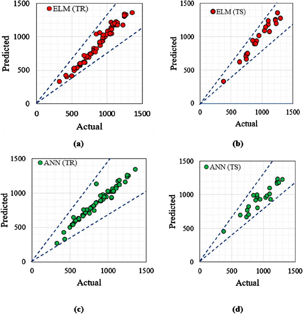
Figure 14. Actual v/s Predicted graph of UBC for model developed (A) ELM (TR) (B) ELM (TS) (C) ANN (TR) (D) ANN (TS).
Taylor’s diagrams depict the training and testing datasets for the ELM and ANN models, respectively. The point closest to the “reference point” signifies the most effective forecasting model as given in the supplementary file as figure c. The training dataset, ANN is somewhat closer to the reference point, whereas ELM is much closer in the testing dataset. Given the larger importance of performance during the testing phase, the ELM model outperforms the ANN model in forecasting ultimate bearing capacity. The accuracy matrix of the developed models for both the training and testing periods has been illustrated in the figure given in the supplementary file as figure d and e respectively. This matrix serves as a visual representation of datasets and serves as an indicator of the prediction capability of any model. During the testing phase, the ELM model shown exceptional predictive capabilities, obtaining over 97% accuracy in almost all seven specified parameters (R, R2, Bias-Factor, NS, VAF, A20-index, and WI). Moreover, the error matrix of the developed models has been portrayed in the figure given in the supplementary fil, indicating that ELM outperforms the ANN model significantly during the testing phase, exhibiting minimal errors in practically all four parameters (WMAPE, RSR, NMBE, and MAPE). Furthermore, during the training period, ELM’s performance improves marginally whereas ANN’s performance improves dramatically A 3-D surface plot is utilized to illustrate the relationship between a response variable and two predictor factors. Figure f in the supplementary file presents these plots, offering a three-dimensional graph that facilitates the examination of acceptable response values and operating conditions. Figures f with sub version (a), (b), (c), and (d) given in supplementary file showcase the impact of % lime, geotextile depth, maximum settlement, and maximum load on UBC. According to the current study, the optimal geotextile depth for the highest ultimate bearing capacity is 0.2D (3 cm) from the footing’s base, the optimal percentage of lime is 5.0% of the dry weight of the silty sand, and the optimal value of UBC is 1,360 kN/m2.
5 Discussion
Experimental methods for determining ultimate bearing capacity (UBC) for a footing are complex and time-consuming, making computer modelling a helpful tool for simplifying this difficult work. The efficacy of a predictive model is gauged through statistical performance parameters and Taylor’s diagram, where closeness to the “reference point” signifies an ideal model. In this study, Taylor’s diagrams were generated for the developed computational models, including ANN and ELM, utilizing both training and testing datasets. The training phase, ANN is slightly closer to the “reference point,” whereas in testing, ELM significantly outperforms. Notably, ELM has better statistical performance metrics, especially during the testing phase. Given the larger weightage of performance in testing, the ELM model outperforms the ANN model in terms of forecasting ultimate bearing capacity.
Accuracy and error matrices play a crucial role in constructing and selecting models with high precision for out-of-sample data. Therefore, it is essential to evaluate the accuracy of models like ANN and ELM before generating anticipated values. This study provides a one-of-a-kind illustration demonstrating the proposed model’s accuracy and inaccuracy. The Error Matrix and Accuracy Matrix both show that the generated ELM model outperforms the ANN model in terms of predictive capability. In contrast to the ANN model, the ELM model showcases a robust forecasting capacity with high precision, attributed to its faster convergence, learning without iteration, and the inclusion of random hidden nodes, ensuring universal approximation ability.
6 Summary and conclusions
The laboratory findings of this study reveal several significant conclusions. First, a novel approach is introduced for effectively utilizing silty sand and lime, offering a practical method to enhance the ultimate bearing capacity of weak soils, specifically silty sand. The research identifies that the optimal geotextile depth is 0.2D (3.0 cm) beneath the base of the square footing. Additionally, it determines that an ideal lime percentage of 5.0% yields the best results, maximizing the ultimate bearing capacity. Remarkably, the ultimate bearing capacity (UBC) of lime-treated and geotextile-reinforced silty sand reaches an optimal value of 1,360 kN/m2, indicating a substantial increase of 258% compared to the UBC of untreated and unreinforced (plain) silty sand, which is approximately 380 kN/m2. Based on the computational results, the study concludes that the developed computer models, namely Artificial Neural Network (ANN) and Extreme Learning Machine (ELM), effectively replicate the outcomes of the laboratory investigations, providing a faster and more cost-effective alternative to experimental methods. This emphasizes the accuracy and reliability of the laboratory data in determining the optimal geotextile depth and lime proportion necessary for achieving the maximum ultimate bearing capacity (UBC). Furthermore, the ELM model demonstrates superior performance over ANN in terms of competency and precision in predicting ultimate bearing capacity. Consequently, the ELM model emerges as a robust and dependable tool for forecasting the UBC of square footings placed on silty sand, reinforced with geotextile, and treated with lime admixture.
Data availability statement
The original contributions presented in the study are included in the article/Supplementary Material, further inquiries can be directed to the corresponding author.
Author contributions
SY: Conceptualization, Data curation, Formal Analysis, Funding acquisition, Investigation, Methodology, Project administration, Resources, Visualization, Writing–original draft, Writing–review and editing. MK: Supervision, Writing–original draft, Writing–review and editing. SI: Supervision, Writing–original draft, Writing–review and editing. FA: Software, Supervision, Validation, Writing–original draft, Writing–review and editing. PS: Supervision, Writing–original draft, Writing–review and editing. AS: Supervision, Writing–original draft, Writing–review and editing.
Funding
The author(s) declare that no financial support was received for the research, authorship, and/or publication of this article.
Conflict of interest
The authors declare that the research was conducted in the absence of any commercial or financial relationships that could be construed as a potential conflict of interest.
Publisher’s note
All claims expressed in this article are solely those of the authors and do not necessarily represent those of their affiliated organizations, or those of the publisher, the editors and the reviewers. Any product that may be evaluated in this article, or claim that may be made by its manufacturer, is not guaranteed or endorsed by the publisher.
Supplementary material
The Supplementary Material for this article can be found online at: https://www.frontiersin.org/articles/10.3389/fbuil.2024.1495366/full#supplementary-material
References
Abtahi, M., Okhovat, N., and Hejazi, M. (2009). “Using textile fibers as soil stabilizers-new achievements,” in First Int and seventh nat Conf test eng. Rasht, Iran: 2009.
Ali, M. A., and Korranne, S. S. (2011). Performance analysis of expansive soil treated with stone dust and fly-ash. Electron. J. Geotechnical Eng. 16 (I), 973–982.
Bose, B. (2012). Geo-engineering properties of expansive soil stabilized with fly-ash. 17(J): 1339–1353.
Bryson, Jr (1961). A gradient method for optimizing multi stage allocation processes. Proceedings of the Harvard University Symposium on digital computers and their applications.
Cancelli, A., Rimoldi, P., and Tongi, S. (1992). “Frictional characteristics of geogrids by means of direct shear and pull-out-tests,” in International symposium on earth reinforcement practice, 29–34. Kyushu, Japan.
Chen, C., Kenli, Li, Duan, M., and Keqin, Li (2017). Big data analytics for sensor-network collected intelligence. Elsevier Inc. doi:10.1016/B978-0-12-809393-1,00006-4
Das, B. M., and Khing, K. H. (1994). Foundation on layered soil with Geogrid reinforcement-effect of a void. Geotext. Geomembranes 13, 545–553. doi:10.1016/0266-1144(94)90018-3
David, E. R., Geoffrey, E. H., and Ronald, J. W. (1986). Learning representations by back-propagating errors. Nature 323, 533–536. doi:10.1038/323533a0
Farley, B. G., and Clark, W. A. (1954). Simulation of self-organizing systems by digital computer. IRE Trans. Inf. Theory 4 (4), 76–84. doi:10.1109/tit.1954.1057468
Fu, Q., Gu, M., Yuan, J., and Lin, Y. (2022). Experimental study on vibration velocity of piled raft supported embankment and foundation for ballastless high speed railway. Buildings 12 (11), 1982. doi:10.3390/buildings12111982
Ghani, S., and Kumari, S. (2021a). Probabilistic study of liquefaction response of fine-grained soil using multi-linear regression model. J. Inst. Eng. India Ser. 102, 783–803. doi:10.1007/s40030-021-00555-8
Ghani, S., and Kumari, S. (2021b). Liquefaction behavior of Indo-Gangetic region using novel metaheuristic optimization algorithms coupled with artificial neural network. Nat. Haz 111, 2995–3029. doi:10.1007/s-11069-021-05165-y
Ghani, S., Kumari, S., and Bardhan, A. (2021). A novel liquefaction study for fine-grained soil using PCA-based hybrid soft computing models. Sadhana 46 (113), 113. doi:10.1007/s12046-021-01640-1
Gu, M., Cai, X., Fu, Q., Li, H., Wang, X., and Mao, B. (2022). Numerical analysis of passive piles under surcharge load in extensively deep soft soil. Buildings 12 (11), 1988. doi:10.3390/buildings12111988
Guram, D., Marienfeld, M., and Hayes, C. (1994). “Evaluation of nonwoven geotextile versus lime-treated subgrade in Atoka County,” in Oklahoma. Transportation research record. Washington, D.C: National Research Council, 7–11.
Huang, G. B., Wang, D. H., and Lan, Y. (2011). Extreme learning machines: a survey. Int. J. Mach. Learn. Cybern. 2 (2), 107–122. doi:10.1007/s13042-011-0019-y
Huang, G. B., Zhu, Q. Y., and Siew, C. K. (2006). Extreme learning machine: theory and applications. Neurocomputing 70 (1-3), 489–501. doi:10.1016/j.neucom.2005.12.126
Huang, H., Li, M., Yuan, Y., and Bai, H. (2023). Experimental research on the seismic performance of precast concrete frame with replaceable artificial controllable plastic hinges. J. Struct. Eng. 149 (1), 4022222. doi:10.1061/jsendh.steng-11648
Huang, Y., Zhang, W., and Liu, X. (2022). Assessment of diagonal macrocrack-induced debonding mechanisms in FRP-strengthened RC beams. J. Compos. Constr. 26 (5), 4022056. doi:10.1061/(asce)cc.1943-5614.0001255
Kaseko, M. S., and Ritchie, S. G. (1993). A neural network-based methodology for pavement crack detection and classification. Transp. Res. Part C 1 (4), 275–291. doi:10.1016/0968-090x(93)90002-w
Kelley, H. J. (1960). Gradient theory of optimal flight paths. ARS J. 30 (10), 947–954. doi:10.2514/8.5282
Liu, L., Moayedi, H., Rashid, A. S. A., Rahman, S. S. A., and Nguyen, H. (2020). Optimizing an ANN model with genetic algorithm (GA) predicting load-settlement behaviours of eco-friendly raft-pile foundation (ERP) system. Eng. Comput. 36 (1), 421–433. doi:10.1007/s00366-019-00767-4
Malhotra, B. R., and John, K. A. (1986). Use of lime-fly ash-soil-aggregate mix as a base course. Indian Highw. 14 (5), 23–32.
McCulloch, W., and Walter, P. (1943). A logical calculus of ideas immanent in nervous activity. Bull. Math. Biophysics 5 (4), 115–133. doi:10.1007/BF02478259
Miura, N., Saki, A., and Taesiri, Y. (1990). Polymer grid reinforced pavement on soft clay ground. Int. J. Geotext. Geomembr. (9), 99–123.
Mughieda, O., Bani-Hani, K., and Safieh, B. (2009). Liquefaction assessment by artificial neural networks based on CPT. Int. J. Geotechnical Eng. 3 (2), 289–302. doi:10.3328/IJGE.2009.03.02.289-302
Pal, K. S., and Ghosh, A. (2014). Volume change behavior of fly ash–montmorillonite clay mixtures. J. Geomechanics 14 (1), 59–68. doi:10.1061/(asce)gm.1943-5622.0000300
Rahman, M., Wang, J., Deng, W., and Carter, J. (2001). A neural network model for the uplift capacity of suction caissons. Comput. Geotech. 28 (4), 269–287. doi:10.1016/s0266-352x(00)00033-1
Sadrossadat, E., Heidaripanah, A., and Osouli, S. (2016). Prediction of the resilient modulus of flexible pavement subgrade soils using adaptive neuro-fuzzy inference systems. Constr. Build. Mater. 123, 235–247. doi:10.1016/j.conbuildmat.2016.07.008
Steinberg, M. (2000). “Expansive soils and the geomembrane remedy,” in Geo-denver 2000 (ASCE)–2000. doi:10.1061/40510(287)31
Xu, J., Wu, Z., Chen, H., Shao, L., Zhou, X., and Wang, S. (2022). Influence of dry-wet cycles on the strength behavior of basalt-fiber reinforced loess. Eng. Geol. 302 (4), 106645. doi:10.1016/j.enggeo.2022.106645
Yousuf, S. M., Khan, M. A., Ibrahim, S. M., Sharma, A. K., Ahmad, F., and Kumar, P. (2023). A comparison of experimental and computational methods for circular footing response on lime-treated geotextile reinforced silty sand. Model. Earth Syst. Environ. 10, 1281–1303. doi:10.1007/s40808-023-01823-1
Yousuf, S. M., Khan, M. A., Ibrahim, S. M., Sharma, A. K., Ahmad, F., and Kumar, P. (2024). A comparison of experimental and computational methods for circular footing response on lime-treated geotextile reinforced silty sand. Model. Earth Syst. Environ. 10, 1281–1303. doi:10.1007/s40808-023-01823-1
Yu, J., Zhu, Y., Yao, W., Liu, X., Ren, C., Cai, Y., et al. (2021). Stress relaxation behaviour of marble under cyclic weak disturbance and confining pressures. Measurement 182, 109777. doi:10.1016/j.measurement.2021.109777
Zaman, M., Solanki, P., Ebrahimi, A., and White, L. (2010). Neural network modeling of resilient modulus using routine subgrade soil properties. Int. J. Geomechanics 10 (1), 1–12. doi:10.1061/(asce)1532-3641(2010)10:1(1)
Zhang, C., Kordestani, H., and Shadabfar, M. (2022a). A combined review of vibration control strategies for high-speed trains and railway infrastructures: challenges and solutions. J. Low Freq. Noise, Vib. Act. Control, 1420035114.
Zhang, W., Li, H., Li, Y., Liu, H., Chen, Y., and Ding, X. (2021b). Application of deep learning algorithms in geotechnical engineering: a short critical review. Artif. Intell. Rev. 54 (8), 5633–5673. ANNEXURE-1. doi:10.1007/s10462-021-09967-1
Zhang, Z., Li, W., and Yang, J. (2021a). Analysis of stochastic process to model safety risk in construction industry. J. Civ. Eng. Manag. 27 (2), 87–99. doi:10.3846/jcem.2021.14108
Keywords: geotextiles, ground improvements, load settlement test, ANN, ELM
Citation: Yousuf SM, Khan MA, Ibrahim SM, Ahmad F, Samui P and Sharma AK (2024) An evaluation of square footing response on lime-treated geotextile-reinforced silty sand: contrasting experimental and computational approaches. Front. Built Environ. 10:1495366. doi: 10.3389/fbuil.2024.1495366
Received: 12 September 2024; Accepted: 02 October 2024;
Published: 18 October 2024.
Edited by:
Jitendra Khatti, Rajasthan Technical University, IndiaReviewed by:
Amit Verma, Indian Institute of Technology (BHU), IndiaMd Shayan Sabri, Indian Institute of Technology Patna, India
Rubi Chakraborty, National Institute of Technology Meghalaya, India
Copyright © 2024 Yousuf, Khan, Ibrahim, Ahmad, Samui and Sharma. This is an open-access article distributed under the terms of the Creative Commons Attribution License (CC BY). The use, distribution or reproduction in other forums is permitted, provided the original author(s) and the copyright owner(s) are credited and that the original publication in this journal is cited, in accordance with accepted academic practice. No use, distribution or reproduction is permitted which does not comply with these terms.
*Correspondence: Furquan Ahmad, ZnVycXVhbmEucGgyMS5jZUBuaXRwLmFjLmlu