 Maxwell Wondolowski
 Alexandra Hain
 Sarira Motaref
 Michael Grilliot
- 1School of Civil and Environmental, College of Engineering, University of Connecticut, Storrs, CT, United States
- 2NHERI Natural Hazards Reconnaissance (RAPID) Facility, University of Washington, Seattle, WA, United States
Masonry retaining walls are prone to bulging and leaning failures which require high accuracy measurements to monitor. Current assessments of retaining walls rely on qualitative visual inspections that inform overall condition ratings. The site and surface conditions of retaining walls make them challenging objects to 3D image with SfM. SfM is prone to radial distortion, doming, which has resulted in research into mitigation strategies. This study assesses the best practices for implementing Uncrewed Aerial Systems (UAS) to conduct Structure from Motion Photogrammetry (SfM) on masonry retaining walls as a more objective, accurate, and accessible means of inspection. The efficacy of doming mitigation strategies when applied to masonry retaining walls was explored in the current study. This was carried out through the duplicate imaging of two sample retaining walls with terrestrial laser scanning (TLS) and SfM. The TLS generated 3D models were used as baselines to compare the trial SfM generated 3D models with CloudCompare. SfM models not initially exhibiting doming displayed an average of 5.8 mm (0.23 in) root mean square error (RMSE) when compared to TLS baselines. The errors in SfM models that exhibited doming were improved with the addition of ground control points, resulting in a 46% reduction in error. Findings and the best practices for SfM image networks and ground control point inclusion for two retaining walls are provided based on results of this research. The benefits and inherent limitations of SfM as used for retaining wall 3D imaging to contribute to the growing applications of SfM in infrastructure inspections are discussed.
1 Introduction
The National Park Service’s Wall Inventory Program (NPS WIP) represents one of the most robust wall inventory initiatives undertaken by a government agency, aiming to define and quantify wall assets in terms of their location, geometry, construction attributes, condition, failure consequence, cultural value, apparent design criteria, and cost of structure maintenance, repair, or replacement (DeMarco et al., 2009). By 2008, over 3,500 retaining walls in 34 national parks in 27 different states across the United States were inventoried (Emeritus Members of the Steering Committee, 2008; NPS, 2015). The inventory of these structures included newly constructed assets to walls over 80 years old (Federal Highway Administration, 2008). Preliminary findings of the NPS WIP indicate that 29% of all retaining wall structures assessed are in of need maintenance, repair, or replacement (Emeritus Members of the Steering Committee, 2008). There are many types of retaining walls such as gravity walls, cantilever walls, and mechanically stabilized earth (MSE) walls. Stone masonry retaining walls are unique in that they are mortarless structures, relying entirely on friction between the faces of interlocking surfaces under self-weight for structural integrity (Clayton et al., 2013). Stone masonry walls make up 70% of all walls assessed in the NPS WIP (CTC and Associates, 2013). The inherent variability of this type of structure makes it challenging to predict performance and draw trends in routine inspections. DeMarco (CTC and Associates, 2013; Anderson Scott et al., 2012), an expert associated with the NPS WIP, indicated that walls were likely overlooked during their inventory due to the structures’ secluded locations and scarcity of as-built records. Isfeld-Corresponding et al. (2016) also shared that damage assessment is a challenge for masonry walls in their analysis of grout injection repairs. Inspections of these structures still rely upon antiquated methods.
In a traditional inspection, an inspector makes a qualitative assessment and later converts it to a numerical rating. This is supported by hand drawings and field measurements (Butler et al., 2016; Hain and Zaghi, 2020). Traditional inspection methods have significant limitations as the collected information is largely subjective, challenging to reproduce with precision, and may vary greatly depending on the individual experience of the inspector. The practice of numeric structural rating also carries the inherent risk of masking critical developing issues within a structure that are balanced out in the rating by overall acceptable performance. Additionally, there is no standardized structural rating scale, further contributing to the ambiguity that these ratings may convey (Butler et al., 2016). Three-dimensional (3D) imaging helps to solve these shortcomings by providing quantitative measurements of an entire structure that enables the detection of growing issues within a structure. Recent advances in 3D imaging technology and computing have lowered costs and improved processing speeds. As a result of these improvements, 3D imaging has become more viable for the inspection of civil infrastructure, including masonry retaining walls. Light distance and ranging (lidar) and SfM are among the most used methods (Oats et al., 2017; Yust et al., 2017; Kaartinen et al., 2022).
Lidar is an active form of 3D scanning that offers high accuracies and is best suited for rapid and large-scale data collection (Gregersen, 2023). Scanning units using lidar based terrestrial laser scanning (TLS) can capture structures with 1.3 mm (0.05 in) accuracies within 27 m (88.6 ft) as compared to total station measurements but at very high costs (Psimoulis et al., 2022). SfM is a passive means of 3D imaging that presents a cost-effective and accessible alternative to TLS with standard SfM equipment costing 10% its TLS counterparts. This is because TLS requires highly specialized and precise equipment to collect data while SfM models can be produced with images taken using virtually any commercially available camera. The greater accessibility of SfM equipment makes it a more approachable method of 3D imaging compared to traditional TLS. While this gap in equipment availability is shrinking as basic lidar sensors now exist in some modern smartphones, their uses for this application are limited. One recent study from the United States’ Federal Highway Administration assessing the use of smartphone based “pocket lidar” for MSE retaining wall assessments found limitations in local accuracy and the ability to monitor defects such as bulging (Corrigan, 2024). While the advent of pocket lidar is a step towards improving the affordability and accessibility to lidar based imaging, the reliable accuracy of TLS justifies the cost in many cases. The implementation of SfM or TLS offers benefits to retaining wall monitoring that are otherwise unattainable using conventional inspection methods. When used properly, the 3D imaging data generated through TLS or SfM is accurate, precise, and reproducible. These technologies can be used to identify cracks and surface abnormalities, track movements over time, and provide detailed sectional slope analysis of retaining wall structures (Butler et al., 2016; Yust et al., 2017; Mohammadi et al., 2019). The identification of such irregularities enables timely and effective maintenance and repair measures to be taken.
In recent years, there have been laboratory and field evaluations using SfM to collect data on retaining walls. Two studies from Oats et al. (2017) and Oats et al. (2019) found SfM to be accurate within 1.5 cm (0.59 in) when compared to total station measurements and that accuracies can be improved with the optimal inclusion of control points. One proof of concept study from Hain and Zaghi (2020) found SfM capable of producing comprehensive 3D models of entire retaining wall structures that can identify local areas prone to failure, providing a firm baseline for subsequent inspections that enable detailed deterioration monitoring. Further work from Wondolowski and Motaref (2024) affirmed that SfM is a useful tool for retaining wall inspections, accurate within 5 mm (0.19 in) in certain retaining wall trials. However, Wondolowski and Motaref (2024) found 3D distortions such as the “banana effect” (i.e., doming) to negatively impact the accuracy of retaining wall surface models in certain portions their study. SfM is known to be prone to issues such as doming that create curved and radial distortions in 3D models (Eltner et al., 2016). This type of SfM distortion is correlated to image calibration, parameterization, the inclusion of Ground Control Points (GCPs) and the geometric configuration of images (Eltner and Schneider, 2018; Magri and Toldo, 2017). Jaud et al. (2018) were unable to fully eliminate doming distortions in their study of linear coastal landforms but saw a reduction in magnitude when optimizing the distribution and density of tie points and GCPs with diverse image orientations and ranges. Nesbit and Hugenholtz (2019) found that the imaging angle has large impacts on the accuracy of SfM results and that the incorporation of oblique images to a nadir only image set will yield improved accuracies, though no decisive optimal combination of angles were determined. While many studies have evaluated means of mitigating this effect in aerial SfM, there is very little research on its impacts to the inspection of vertical structures such as retaining walls.
This study evaluates the efficacy of close-range, manually flown, aerial based SfM for retaining wall 3D imaging. A specific focus was evaluating the prevalence and mitigation of doming distortions on retaining wall imaging using SfM modeling. For this purpose, the field study of two masonry retaining walls are presented. Data was collected using a TLS unit and an uncrewed aerial system (UAS) for SfM. SfM was assessed for both accuracy and feasibility by considering site access constraints as well as the cost and availability of the necessary equipment. The accuracy of close-range SfM measurements were determined by comparing them to ground truth measurements established using TLS in this paper. SfM accuracy was measured using Cloud to Cloud (C2C) comparisons between SfM point clouds and ground truth TLS point clouds. The reliable accuracy of TLS makes it a great candidate for establishing ground truths for this type of comparison. TLS has been used in this capacity in recent literature assessing infrastructure inspection techniques (Chen et al., 2019; Byrne et al., 2017). The time required for both field data collection and post-processing was recorded to provide insight into the feasibility of implementing SfM-based inspection protocols at scale.
2 Materials and methods
This section outlines the methodology used to assess the performance of SfM for the inspection of retaining walls using TLS as a baseline. The materials and methods are structured to report a comprehensive view of the experiment’s design, imaging technologies implemented, data collection procedures deployed, and data processing steps. The methods described in this section are intended to be replicable and relevant to asset managers aiming to integrate 3D imaging into routine retaining wall inspections.
2.1 Study overview
This work presents a controlled field trial comparing SfM and TLS methods on two representative retaining walls. The section begins by outlining the objectives of the investigation, followed by a description of the selected site characteristics. This overview provides essential context for the methodological approach described in the remainder of the section, clarifying the rationale behind the experimental design.
2.1.1 Objectives
A field trial was designed to accomplish three main objectives, 1) assess the accuracy of SfM compared to a TLS baseline 2) evaluate the doming effect in SfM measurements of two different masonry wall types, and 3) develop preliminary guidelines of best practices for 3D imaging retaining walls. Two sites were imaged using TLS and aerial SfM photogrammetry. TLS-generated models served as the reference against which SfM models were directly compared. The study also assessed the practical benefits and drawbacks of using each imaging method. Findings of this study may assist 3D imaging technicians to make informed decisions when choosing inspection protocols for a variety of retaining wall inspections.
2.1.2 Overview of sample retaining walls
Site 1 looked at a 24.7 m (81 ft) section of a 1.5 m (5 ft) tall dry-stone masonry retaining wall. Figure 1A shows an overall view of the wall while Figure 1B shows a close up of the wall surface. This structure had a dynamic surface, typical of dry-stone masonry, and was selected as a representative structure of the multitude of dry-stone masonry walls that require inspection and maintenance in the United States. This site had no vegetation impacting the study area. While the overall structure was curved the section of the wall being studied had negligible curvature. It was investigated if the unique surface of the dry-stone masonry wall at Site 1 yields more accurate SfM results due to decreased doming effects.
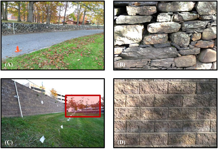
Figure 1. (A) Wide view of Site 1, (B) Close-up view of Site 1, (C) Wide view of Site 2, (D) Close-up view of Site 2.
Site 2 examines a masonry retaining wall constructed of uniform concrete masonry units as shown in Figures 1C,D. This study collected data on a 24.7 m (81 ft) long section of the 3.1 m (10 ft) tall structure. This type of wall with a uniform surface was selected to assess the prevalence of SfM distortions on a structure. In addition, the impact of the site’s vegetation on the overall quality of the SfM models produced was studied. Trees partially obstructing a portion of the wall on Site 2 are shown highlighted in red in Figure 1C. These trees presented physical obstacles for lidar and SfM data collection and casted shadows across the wall for the duration of the experiment.
2.2 Overview of imaging technologies
This section provides background on the functions and applications of each imaging method utilized in the study. It also details the specific equipment and software employed during data collection and processing.
2.2.1 Terrestrial laser scanning (TLS)
Terrestrial laser scanning (TLS) refers to a ground based and typically tripod mounted implementation of lidar. In principle, lidar works by shooting pulsed beams of light at an object and measuring the amount of time it takes for that light to travel and reflect back to a sensor within the scanner, yielding something known as a time-of-flight measurement, shown in Equation 1 (Neoge and Mehendale, 2020).
Equation 1 uses the time between the laser pulse and measured return (∆T) in combination with the constant speed of light (c) to derive the distance to the target (D). Lidar scanners create 3D models of the objects being scanned by repeating this process a number of times to measure individual points on the surface of the object which are then cataloged and displayed in a 3D model known as a point cloud (Neoge and Mehendale, 2020; Raj et al., 2020). These repeated measurements with multiple returns often allow lidar to penetrate or filter out vegetation in the scans (Liao et al., 2021; Brodu and Lague, 2012).
2.2.2 TLS equipment
The Leica RTC360 TLS unit was chosen to capture high quality 3D models of the walls to serve as the baseline for the accuracy comparison in this study. It was selected as a baseline due to its high accuracy and reliable usage in modern engineering applications (Moberg, 2023). The RTC360 produces point clouds with 360° horizontal and 300° vertical fields of view with point accuracies of 1.9 mm at 10 m (0.07 in at 32.8 ft) and 2.9 mm at 20 m (0.11 in at 65.6 ft) (Leica Cyclone Register 360, 2025). The scans are collected at a maximum point density of 3 mm (at 10 m). The scanner is also capable of real-time point registration (Leica RTC360, 2025). A preliminary 3D model can be created and displayed which enables user to make decisions to improve the quality of collected data while still in the field. These features and specifications are invaluable to a 3D imaging technician but come at a high cost compared to SfM equipment. The RTC360 costs $75,000 (2025 pricing) which includes only the scanner and its processing software, Leica Cyclone Register 360.
2.2.3 Structure from motion photogrammetry (SfM)
SfM is a 3D imaging method that constructs a 3D model by triangulating the position of features captured by overlapping images of an object (Eltner and Sofia, 2020). SfM software, such as RealityCapture or Pix4D, accepts an input set of images captured of an object from varying, overlapping angles and produces point clouds. SfM has a critical limitation as it needs scaling information. The point clouds generated contain only relative geometry that must be assigned scale using objects of known dimensions within the object’s region (Mubanga, 2025).
2.2.4 SfM equipment
The DJI Mini 3 Pro camera drone was chosen to capture images to assess the quality of manually flown aerial SfM in this study. This drone takes images with a maximum quality of 48 megapixels. It offers the advantage of Global Navigation Satellite System (GNSS) connectivity, enabling images to be automatically georeferenced (DJI Mini 3, 2023). It is also equipped with obstacle detection systems that can aid inspectors in safe operation by warning them of obstacles relative to the UAS. The Mini 3 Pro retails for $600 and was chosen to represent a low-cost drone capable of capturing high quality images that 3D imaging technicians might consider purchasing to capture 3D models of subjects that are challenging to access with TLS and traditional cameras. It is not only low cost but also compact, with a takeoff weight of 249 g (8.7 oz) and only 25 × 362 × 70 mm (9.9 × 14.2 × 2.7 in), making it highly maneuverable in tight quarters. This study used RealityCapture for all SfM model processing. An unlimited license for RealityCapture can be purchased for $3,750 (2025 pricing) though pay-per-input pricing is also available (RealityCapture, 2024).
2.3 Data collection
The following section outlines the workflows used to collect TLS and SfM data. TLS data was collected first on each site immediately following site preparation with alignment targets, image locations, and scale rods. This ensured that accurate point clouds could be collected and used as ground truth. Images for SfM reconstruction were then collected at predetermined locations.
2.3.1 TLS and GNSS data collection
The collection of quality TLS data was critical in the current study as it served as the baseline upon which all conclusions on SfM accuracy were drawn. To ensure highly accurate baseline 3D models, the Leica RTC360 terrestrial TLS scanner was used to measure each wall at 3 separate stations. TLS scans were collected 4.6 m (15 ft) from the subject’s surface to maximize the accuracy of the RTC360 (Leica RTC360, 2025). This also assured that critical details were captured at a maximum of 45-degree oblique angles to minimize distortions in individual lidar returns (Laefer et al., 2009). These stations were carefully positioned so the full structures could be imaged without any blind spots. All TLS data was also collected well within 10 m (32 ft) of the structure to ensure the baseline data was accurate to 1.9 mm (0.07 in). Full dome scans were captured at each station on both sites. Two redundant scans were collected at each station on Site 2 so that the unavoidable foot traffic through the study region could be effectively removed from the final TLS cloud. TLS data collection required approximately 30 min per site. This time included the initial setup of the equipment, the collection of six total scans each taking approximately 3 min, repositioning of the TLS unit between stations, and the breakdown and stowage of the equipment. The position of each scanning station was documented using a Leica GS18T GNSS antenna. All TLS and GNSS equipment used in this study was rented from the National Science Foundation’s Natural Hazards Engineering Research Infrastructure RAPID facility (NSF NHERI Rapid Facility, 2025).
2.3.2 SfM data collection
The data collection plan was developed as shown in Figure 2A. This plan shows the locations of TLS scans, image collection passes, alignment targets, and scale rods. While Figure 2A only shows the plan for Site 2, the same procedure was executed on both sites. Figure 2A notably includes the path of two image collection passes. The first path, shown in light blue, collected images at a range of 3.04 m (10 ft) from the wall. Within this “close pass” photos were taken of the wall every 0.91 m (3 ft) horizontally and vertically. The “far pass” shows the path where images were collected at a range of 9.14 m (30 ft) from the wall. At this range, images were spaced 2.74 m (9 ft) horizontally and 1.82 m (6 ft) vertically. All image locations were laid out and flagged prior to data collection to ensure consistent spacing. To ensure a robust SfM model, images of the subject must be captured at many overlapping angles. Image spacing was selected to provide sufficient image overlap for optimal SfM accuracy (Wang et al., 2022; Obanaw et al., 2020). Images were collected at vertical angles normal to the surface of the wall and with ±5, ±15, and ±30-degree offsets from normal to investigate the impact that oblique views of the subject have on the prevalence of doming. Additional images were collected of the scale rods at close range to ensure sufficient data quality for SfM model scaling. SfM data collection on each site took approximately 5 h. The collected data was employed to generate four distinct SfM models for each site. This suggests that SfM data collection intended solely for inspection purposes can typically be completed in an estimated 1–2 h per site.
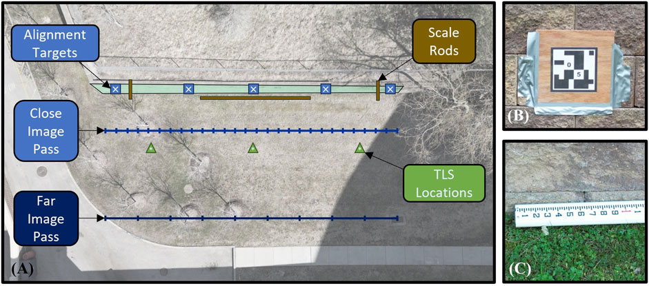
Figure 2. (A) Data Collection Plan for Site 2, (B) Close-up of Alignment Target, (C) Close-up of scale rod.
It is critical to carefully consider the requirements of both the site and imaging method prior to collecting data for 3D imaging. This study included the use of alignment targets on the subject wall, shown in Figure 2B. These alignment targets are useful to the user during the data processing phase of SfM as they present hard points that can be used as tie points and control points within the SfM model. In this context tie points are visibly identifiable points within the subject region that can be manually selected from multiple camera angles. These tie points help inform the SfM model and improve its overall accuracy. These targets can also be used as temporary GCPs by assigning them local coordinates within the SfM model that were collected through other means (e.g., survey or TLS).
Scale rods are included in this study to provide artifacts of known dimensions within the subject region to scale the SfM models and shown in Figure 2C. A pivotal distinction between TLS and SfM-generated 3D models lies in the inherent inclusion of scale when utilizing TLS, whereas SfM lacks automatic scaling capability. SfM models are scaled during data processing by manually creating tie points to define objects of known distance. Survey scale rods were used to scale the SfM models. Additional images were captured of the scale rods to ensure sufficient image coverage to enable the creation of manual tie points for scaling.
2.4 Data processing
This section details the steps taken to process TLS and SfM data into point clouds. Preliminary TLS data processing took place in the field during data collection and was later finalized in Leica’s companion software. SfM data processing followed a multi-step workflow that included camera calibration, image alignment, and manual refinement. Post-processing steps including trimming, registration, and cloud comparisons are also detailed below.
2.4.1 TLS data processing
Processing TLS data collected with Leica’s RTC360 scanner began in the field during data collection. Leica’s Cyclone FIELD 360 software allowed for automatic pre-registration and alignment when operating the RTC360 through a paired companion device (Leica Cyclone FIELD 360, 2024). An iPad running FIELD 360 was used to pre-register and align TLS data as it was collected. These pre-registered scans were then imported into Lecia’s Cyclone REGISTER 360 software for fine tuning and alignment checks (Leica Cyclone REGISTER360, 2025). TLS data processing took less than 1 h per site. TLS data was exported from REGSITER360 as .las files, an industry standard file format for exchanging TLS point cloud data. These files were used as baseline models to assess the accuracy of SfM.
2.4.2 SfM data processing
RealityCapture was used to process images into 3D models using SfM in this study (RealityCapture, 2024). SfM data processing began by importing a selection of images into the software. RealityCapture then calibrated each image using data about the camera parameters embedded in each file. This research made use of the Brown polynomial distortion model included in RealityCapture for camera registration and calibration (Distortion Model, 2024). The distortion model corrects camera distortion by considering the impacts of radial and tangential decentering distortions that may be present in each image (Brown, 1965). Equation 2 shows the image calibration model that was used to calculate the undistorted image point (
RealityCapture performed bundle adjustments of input images using the Brown model to correct distortions. The distortions are the result of lens manufacturing imperfections that shifted the optical axis of the lens off its geometric center (Wang and Liu, 2022; Remondino and Fraser, 2006). Table 1 displays a sample of used lens calibration parameters by RealityCapture during SfM processing. This table includes information about the calibrated focal length (f), 4 degrees of radial distortion (k1-k4) and 2 degrees of tangential distortion (t1-t2).
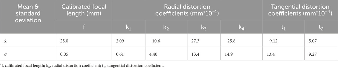
Table 1. Brown 4 with tangential 2 lens calibration parameters.a
After camera calibration, initial image alignment was executed with RealityCapture’s image alignment algorithm. This algorithm oriented all input images in 3D space and generated a sparse point cloud 3D model. The sparse point cloud was improved through the addition of manual control points within the model space. Both manual tie points and GCPs were used to supplement the SfM alignments. Manual tie points were created by selecting a single point within the model from multiple input cameras. To improve the accuracy of SfM, manual tie points on each alignment target and along each scale rod were used. Figure 3 provides a representative view of a sample manual tie point in RealityCapture. The location of this manual tie point can be seen in the collection of images on the right side of Figure 3. Distance constraints between manual tie points on scale rods of known offsets were incorporated to scale each model.
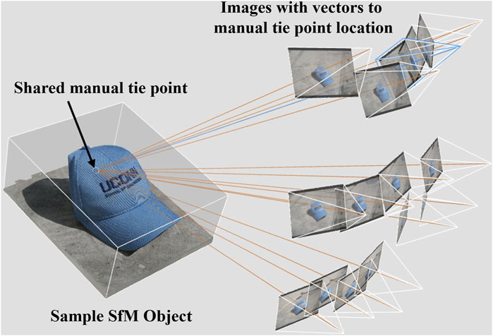
Figure 3. Representative view of manual tie points in SfM data processing with RealityCapture.
Manual tie points can also be treated as GCPs to further improve accuracy by assigning them 3D coordinates within the model space. The assigned 3D coordinates for GCPs must be obtained through some other means of measurement and are often created using survey, GPS, or even lidar. While GCPs are often permanent fixtures of known locations, the GCPs created on the alignment targets in this study were temporary. Temporary GCPs can still be used to refine SfM reconstructions if reliably measured, avoiding the need for protected permanent installations. Certain portions of presented analysis used 3D coordinates at alignment targets from the baseline TLS models to further augment the associated SfM models.
Realigning the models was the final steps of creating SfM models after sufficient information has been added by the user, including manual tie points, distance constraints, and GCP coordinates, when applicable. The realignment of the model produces another sparse point cloud that incorporates all the provided information with improved geometric and spatial accuracy. Next, RealityCapture’s model generation tool was used to generate the final 3D model as a densified point cloud. The colorized dense point clouds were exported as.las files for further analysis. Start to finish data processing for each SfM model took approximately 6–18 h. The creation of manual tie points in each model is the most actively time-consuming step of the process, meaning that it requires the user’s full attention for the duration of this processing step. This took approximately 1–2 h per model. SfM reconstructions are computationally demanding and required 4–16 h of passive processing time per model in this study.
2.4.3 TLS vs. SfM CloudCompare analysis
CloudCompare, an online and open access software solution for point cloud operations, was used to analyze the 3D models created (CloudCompare, 2023). In all global accuracy comparisons, TLS point clouds were used as baseline ground truths to compare different SfM point clouds against. This process started by roughly trimming all point clouds to remove unnecessary data outside of the study area at each of the subject walls. Models were aligned by only their scale rods to help improve model registration quality by lowering the potential of inconsistencies in model trimming that could create areas of localized minimum error. Alignment was achieved with CloudCompare’s “Fine-Registration” tool which uses an iterative closest point algorithm that works by selecting representative points of each input point cloud and iteratively matching common points between clouds (Li et al., 2021; CloudCompare, 2015).
The differences between aligned point clouds were measured in this study with cloud-to-cloud (C2C) comparisons. C2C comparisons work in CloudCompare by iterating through each point in a “reference cloud” to determine the nearest neighboring point in a “compared cloud” and assign the absolute distance between these two points in a scalar field of points from the “reference cloud.” TLS point clouds were treated as baseline measurements and were used exclusively as the “reference clouds” in this study’s analysis of the SfM “compared clouds.” CloudCompare allows the resultant scalar fields of C2C comparisons to be viewed as colored displacement maps, enabling the evaluation of trends in error. It is important to realize that due to the inner workings of the C2C algorithm the output contains only absolute distances agnostic to the direction of displacement.
Surface roughness was measured in this study to provide additional insights into the capabilities of SfM and TLS to accurately capture the geometry of retaining walls. This analysis differed from the above description of global C2C comparisons as it provided information on the fidelity of local surfaces rather than the global accuracy of each retaining wall model. The alignment targets on each wall were chosen for this analysis and isolated in each point cloud. These targets were chosen for this step of analysis given the flat and smooth nature of their surface. A flat 0.25 m × 0.25 m (0.82 ft × 0.82 ft) plane was generated in CloudCompare to serve as the basis of this surface roughness analysis. A planar point cloud was then generated by subsampling this plane at a density of four million points/m2. This high-density plane was then aligned to the isolated alignment targets with CloudCompare’s fine-registration tool. The planar point cloud provided a ground truth approximation of the flat alignment targets. C2C comparisons were then conducted between the alignment target sections of each point cloud in this study and their corresponding planes. The results of this comparison were used to determine fidelity of local surfaces generated by each imaging method.
Assessments of point distribution were conducted on all point clouds. This analysis was conducted using the “Compute Geometric Attributes” toolbox in CloudCompare. Scalar fields of precise point density were calculated by measuring the number of neighboring points within a spherical radius of each point (CloudCompare, 2022). A radius of 5.0 cm (1.96 in) was used in these calculations in line with a similar analysis conducted by Chen et al. (2019) in their study of SfM imaging for bridge inspections.
2.4.4 Lighting analysis
An analysis of lighting conditions was conducted in response to the prevalence of shadows in images that were noticed during SfM data processing. Lighting conditions in all images used for SfM reconstruction were analyzed to assess the potential impact of the dynamic lighting present during data collection on model quality. Each image was first converted to grayscale using tools the Python Imaging Library Pillow (Lundh and Clark, 2025). Each pixel was assigned a value from 0 to 255 representing its original RGB brightness. The mean of grayscale pixel values was then calculated to quantify the overall brightness of each image. These image-level means were then averaged across all images used for each SfM reconstruction to yield model-wide metrics of brightness. The percentage of pixels below a grayscale intensity threshold of 134 was computed for each image to estimate the prevalence of shadows. This threshold for shadow detection was determined by averaging the Otsu thresholds of each SfM image set using the scikit-image Python library (Van Der Walt et al., 2014; Aghamaleki, 2022).
3 Results
The results of quantitative analysis compare the accuracy of manually flown UAS based SfM models to TLS baseline models are presented in this section. The impact of doming on the results are evaluated and their cause and potential measures for mitigation are discussed. The feasibility of manually flown UAS data collection for SfM retaining wall inspection are further explored in a discussion of site limitations, equipment pricing and availability, training requirements, and on-site time requirements.
3.1 3D visualizations
Fourteen distinct 3D models of two retaining walls were generated to assess the accuracy of the imaging methods employed. A naming convention containing information about each model is established in Table 2 and is used to label models throughout the results section. This naming convention includes information on the site, imaging type, and types of images included in SfM reconstructions. For example, S1-TLS refers to model for Site 1 captured using TLS and S2-SFM-GCP-0-5 refers to the model for Site 2, captured with SfM, using GCP coordinates, created using images captured 0° and ± 5° to the surface. All models exist in the form of point clouds, discrete collections of points in 3D space that together form the geometry of 3D models.
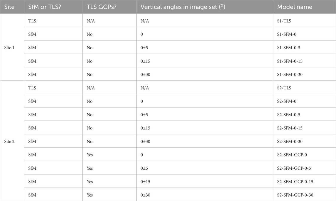
Table 2. 3D model naming convention.
Table 3 displays information on storage size, point count, and point density for all point clouds and input images for the SfM-created models. The structure on Site 2 was taller than the structure on Site 1 which required the addition of a third altitude pass of image, resulting in an overall greater count in images. The slight variation in image count between sets on Site 2 is due to the exclusion of certain images due to excess blurring caused by suboptimal lighting conditions. As a point of comparison, the trimmed TLS clouds used in this study contained 15,677,189 and 24,000,336 points for Site 1 and Site 2, respectively. Site 1 TLS was stored in a 0.40 gigabyte (GB) .las file and Site 2 TLS data was stored in a 0.61 GB .las.
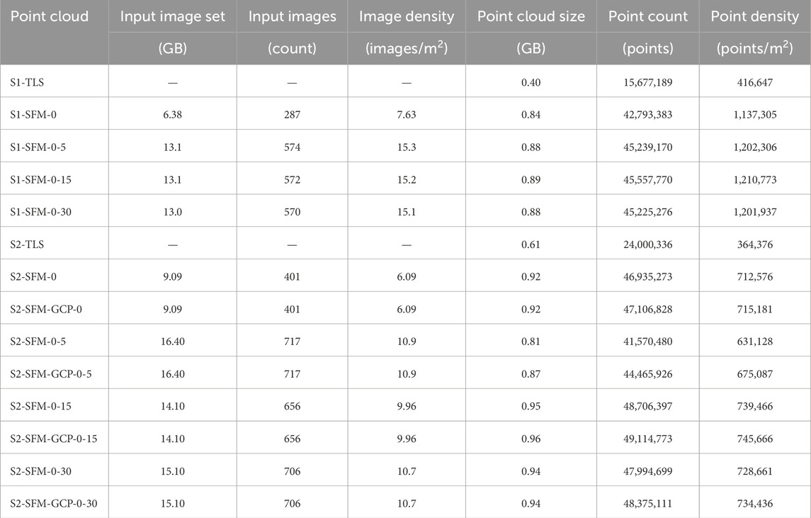
Table 3. Data and point cloud density.
Figure 4 shows a view of two 3D models of the same region from Site 1. Figures 4A,B was generated using TLS while Figures 4C,D was generated using SfM. Figure 4B showcases the uniform, grid-like pattern of point distribution characteristic of TLS systems. The TLS point cloud in Figure 4A is 398 MB and contains 416,647 points/m2 of wall and the SfM point cloud in Figure 4D is 835 MB and contains 1,137,305 points/m2 of wall.
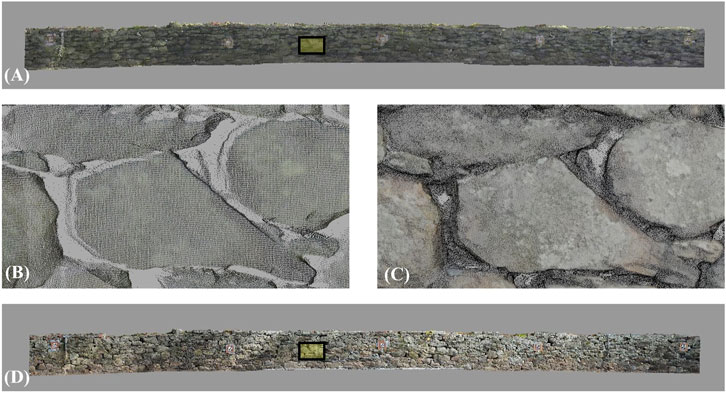
Figure 4. Sample views of 3D models on Site 1: (A) TLS, (B) TLS close-up, (C) SfM close-up, (D) SfM.
Figure 5 shows a view of the TLS baseline and one SfM model of Site 2. The TLS point cloud in Figures 5A, B is 609 MB and contains 364,376 points/m2 of wall and the SfM point cloud in Figures 5C, D is 916 MB and contains 712,576 points/m2 of wall. The same difference in point distributions can be observed when comparing the close-up views of the TLS and SfM point clouds. Detailed information regarding the data density of all point clouds in these models can be found in Table 3. Comparisons between the fidelity of SfM surfaces on Site 1 in Figure 4C and SfM surfaces on Site 2 in Figure 5C suggest that SfM was more effective on the drystone masonry surface of Site 1. The distinctive surface at Site 1 featured numerous identifiable characteristics that enhanced the performance of SfM feature detection algorithms. This trend is also evident in Table 3 which shows that the average point density of SfM models on Site 1 was 1.67 times larger than that of the average point density of SfM derived point clouds on Site 2.
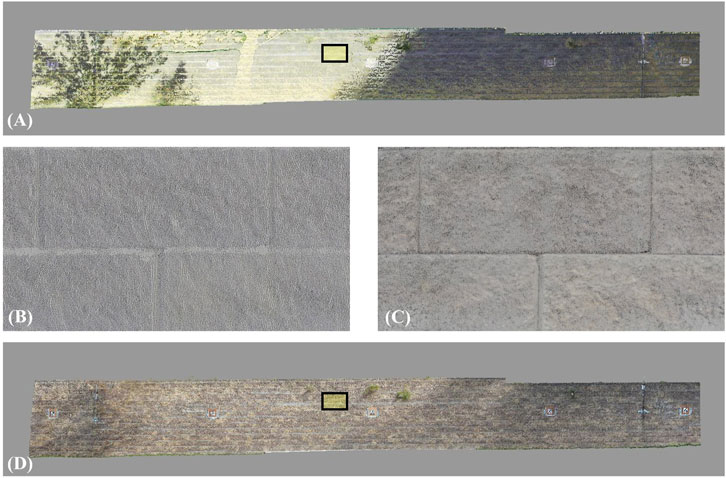
Figure 5. Sample views of 3D models on Site 2: (A) TLS, (B) TLS close-up, (C) SfM close-up, (D) SfM.
Sharp shadows can be observed cutting across the subject surface in Figure 5A. While these shadows were present during the data collection of both the TLS and SfM data collection, they show most prevalently on the TLS model. This is likely because all TLS data was captured within a 20-min window, meaning that all three scan stations saw these sharp shadows in relatively consistent locations. Two scans were collected at each station, each taking approximately 3 min, before the scanner was moved and relevelled, taking approximately 2 min. This allowed enough time for the edges of the shadows to shift between individual scans without much change in the overall shadows. The green discoloration visible around some of the shadows in Figure 5A can be attributed to these slight shifts in shadows overlapping between subsequent TLS scan locations. While there are remnants of the shadows in Figure 5D they are far less prominent than in the TLS scan because SfM data collection was collected over the course of hours. This means that SfM images captured a variety of lighting conditions on the wall which were somewhat averaged out in the creation of SfM 3D model. This dynamic lighting is known to present challenges for accurate SfM reconstruction that will be addressed in the coming discussion of results from the lighting analysis. The discrepancy in data collection time is a key difference between the two imaging methods and will be discussed further in later sections of this paper.
3.2 Surface roughness
Figure 6 shows the results of the surface roughness analysis conducted on all point models in this study. The surface roughness analysis produced C2C comparisons that represent the differences between an artificially generated plane and the hypothetically planar surface of the center alignment target in each point cloud. TLS surfaces are observed to have a more uniform distribution of error compared to SfM generated surfaces in Figure 6. The RMSE, mean, and standard deviation of these results are shared in Table 4. TLS surfaces are observed to be slightly rougher than SfM surfaces with an average error between the two TLS surfaces of 0.41 mm and an average error between all SfM surfaces of 0.37 mm.
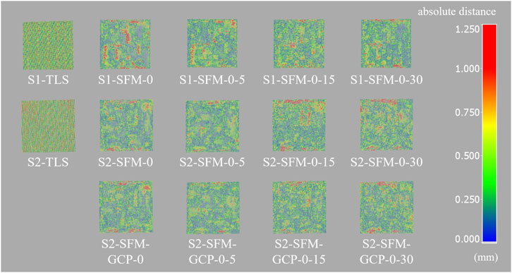
Figure 6. Surface roughness on central alignment target.
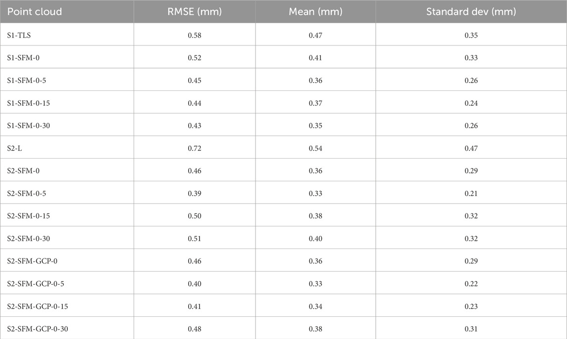
Table 4. Surface roughness.
3.3 Point distribution
The results of the point distribution analysis are shown in Figures 7A–D. The color ramp displays a discrete count of neighboring points within a 5 cm (1.96 in) spherical radius. TLS models are shown to have nonuniform distributions of points along the span of each wall with higher density at the ends and center. This was expected given the positioning of the three TLS scan stations, shown previously in Figure 2A. The TLS models have higher point density on segments of the walls’ surfaces more orthogonal to the TLS scan locations due to the radial propagation of TLS measurements. The outline of a tree can be seen in Figure 7C. This portion of the wall was occluded by vegetation in 1/3 scan locations, resulting in decreased density on that portion of the wall. SfM models are shown to have relatively uniform point distributions except for areas surrounding the scale bars. Non-uniform density around the scale bars was a result of the additional images captured of the scale bars. These additional images were included in SfM processing to ensure sufficient coverage for scaling the models.
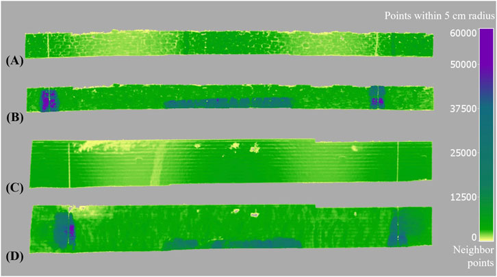
Figure 7. TLS vs. SfM point distribution by site: (A) S1-TLS, (B) S1-SFM-0, (C) S2-TLS, (D) S2-SFM-0.
3.4 Site 1 SfM accuracy comparisons
Figure 8 shows the accuracy of four SfM models of Site 1 as scalar fields displaying the error across the entire structures and a combined histogram of measured error. The C2C error in S1-SFM-0 which was created exclusively with images captured perpendicular to the surface plane of the wall is shown in Figure 8A. It is evident that S1-SFM-0 had a higher magnitude of error than the rest of the models at Site 1 which was expected and due to the fact S1-SFM-0-5, S1-SFM-0-15, and S1-SFM-0-30 (Figures 8B–D) all had more input images with the addition of oblique angles. It is important to note that there are no visibly discernible patterns of error between these four models that are indicative of doming.
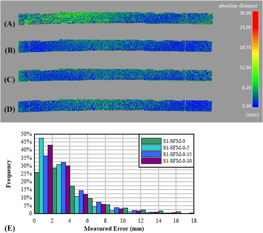
Figure 8. Site 1 Full-Wall C2C accuracy of SfM compared to TLS ground-truth: (A) S1-SFM-0, (B) S1-SFM-0-5, (C) S1-SFM-0-15, (D) S1-SFM-0-30, (E) summative histogram.
Figure 8E shows the accuracy of four SfM models in a histogram format. The x-axis in this histogram is the magnitude of measured error and the y-axis is the frequency that each magnitude of error occurred in each model. The further left the peak of a model’s error distribution curve, the more accurate that model can be considered. The most accurate SfM model for Site 1 is shown to be S1-SFM-0-5 with a RMSE of 4.8 mm (0.19 in).
3.5 Site 2 SfM accuracy comparisons
Figure 9 presents the accuracy of the four SfM models from Site 2. C2C results in Figures 9A–D show much higher levels of error at Site 2 when compared to the results of Site 1. The consistent radial patterns of error in these models are consistent with that of doming distortion as it appears in retaining walls. This was somewhat anticipated to be present in Site 2 as it is a large relatively uniform surface, making it more susceptible to doming distortion. It is evident that doming is impacting all four of the SfM models assessed on Site 2.
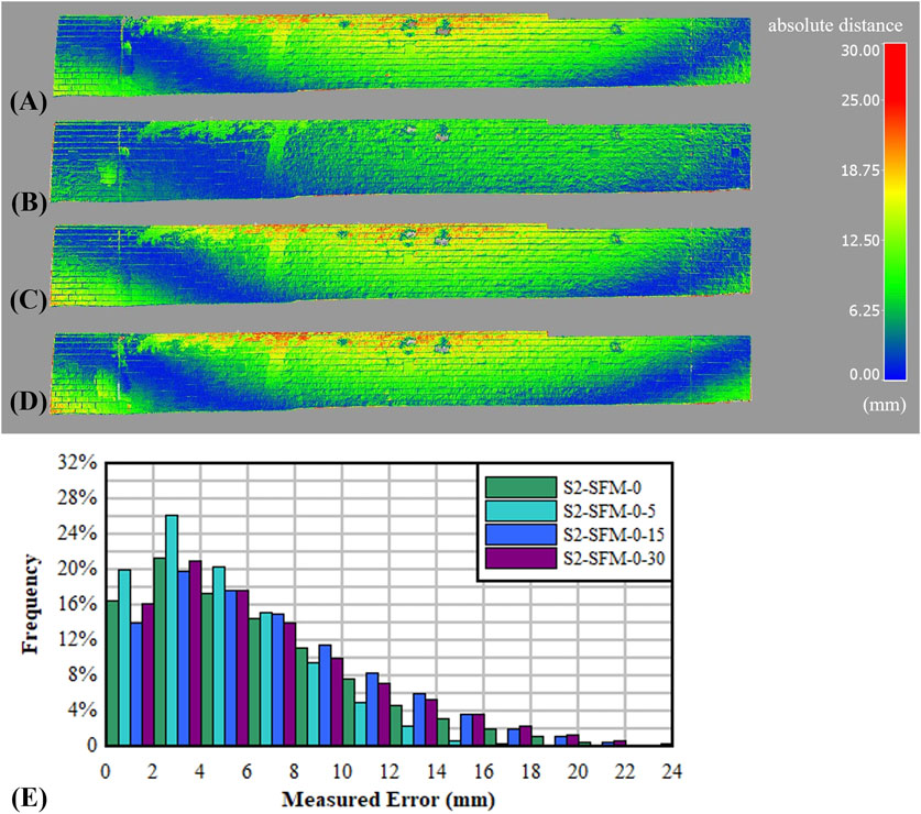
Figure 9. Site 2 Full-Wall C2C accuracy of SfM compared to TLS ground-truth: (A) S2-SFM-0, (B) S2-SFM-0-5, (C) S2-SFM-0-15, (D) S2-SFM-0-30, (E) summative histogram.
Figure 9E, a histogram representation of the scalar fields for site 2, further exemplifies the impacts of doming in these SfM models. The magnitude of error shown on Site 2 in Figure 9E is consistently greater than what was observed on Site 1. The distribution of error is also consistent with a form of model wide distortion such as doming rather than localized regions of high error. S2-SFM-0-5 is shown to be slightly more accurate than the rest with an RMSE of 6.1 mm (0.24 in).
Site 2 had special characteristics that posed potential issues for accurate SfM capture. Firstly, the structure was not a dry-stone masonry retaining wall. Its concrete surface was uniform with few distinguishing features. This type of surface is more challenging to measure accurately with SfM which relies on feature detection for 3D model creation. Secondly, Site 2 had challenging lighting conditions. The collection of all SfM data for this study took place over the course of multiple hours during a day with dynamic cloud cover. This situation created sharp shifting shadows that moved across the wall throughout data collection. A moderate correlation between the presence of these shadows and an increase in SfM error was observed. Site 2 also had a large warehouse structure directly adjacent to it that cast an overall darkness over the structure as daylight hours waned later in the experiment. This created discrepancies in overall image brightness between different images. There were a number of images captured in low light that were removed from the data set due to motion blur created by abnormally long shutter speeds that were meant to account for the lower lighting. The combined effects of surface uniformity, dynamic shadows, and low lighting contributed to the 1) prevalence of doming in Site 2 and 2) the significant difference in error as compared to Site 1.
3.6 Site 2 SfM GCP improvements
A known method of mitigating doming distortions in SfM is through the inclusion of GCPs with 3D coordinates determined outside the SfM processing (Eltner and Schneider, 2018). While this practice does not remove the distortion all together, it can decrease the magnitude of the error produced by doming. This practice was implemented in the analysis and the results are shown in Figure 10. In an effort to improve the quality of SfM results on Site 2, GCP coordinates were pulled from the baseline TLS cloud at each alignment target and assigned to the manual tie points created at those targets within each SfM model. GCP coordinates are commonly collected with total station measurements though TLS was used for its availability. The models were realigned and regenerated, now with the assistance of TLS captured GCP coordinates on the five alignment targets spaced along the structure.
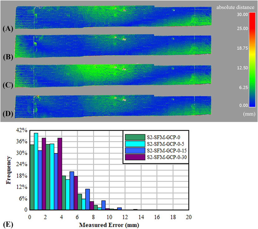
Figure 10. Site 2 Full-Wall C2C accuracy of SfM compared to TLS ground-truth: (A) S2-SFM-GCP-0, (B) S2-SFM-GCP-0-5, (C) S2-SFM-GCP-0-15, (D) S2-SFM-GCP-0-30, (E) summative histogram.
Figures 10A–D shows a dramatic improvement in accuracy with the addition of GCP coordinates to the Site 2 models. All four models exhibit approximately half the amount of error as they were prior to GCP addition yet still show evidence of doming in their distributions of error. Figure 10E shows that the overall accuracy of these four models has been improved.
3.7 Comparison of results
The RMSE and mean of the error in C2C comparisons have been tabulated in Table 5 alongside the lighting metrics of all SfM models. Alignment target error is also shown in this table, which represents the measured difference between the location of the center of alignment targets in the ground truth TLS point cloud and each corresponding SfM model. Though the same trends in errors are observed between the full wall comparisons and alignment target, the overall magnitude of error is higher in the point-point comparisons of the alignment targets. Higher error can be attributed to insufficient data density leading to the imperfect selection of center points on alignment targets. The effects of doming on Site 2 can be observed in the substantial increase in C2C and alignment target error in Table 5 when compared to Site 1. The mitigation of C2C and alignment target error on Site 2 by inclusion of GCP coordinates is also evident.
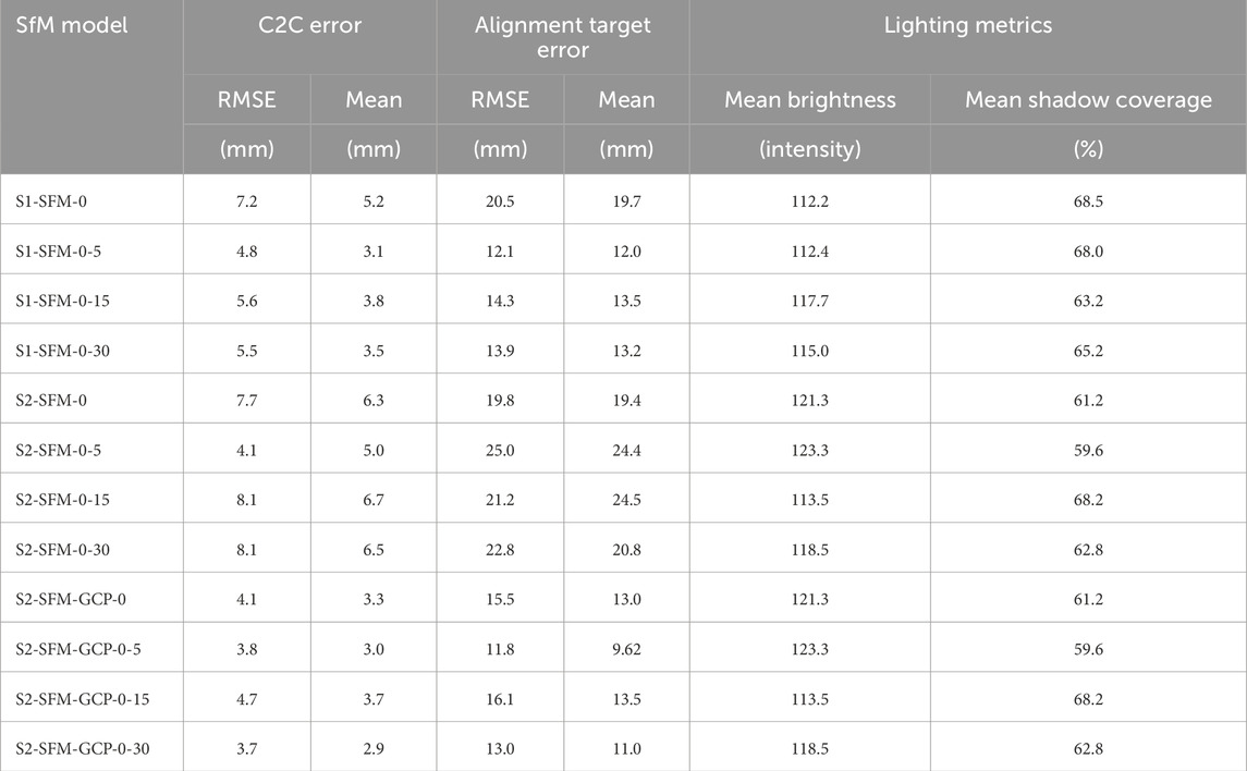
Table 5. SfM error summary.
Table 5 also shares the results of the lighting analysis conducted on images used in SfM reconstructions. On Site 1, there was minimal correlation between C2C error and image brightness (r = −0.24) or shadow coverage (r = 0.31). A trend was observed in the results from Site 2 where dimmer images with heavier shadows were associated with higher C2C error. This was shown by a moderate correlation between C2C errors on Site 2 and image brightness (r = −0.39) and shadow coverage (r = 0.37). The differences in correlation strengths between the two sites can likely be attributed to the differences in their lighting conditions. Site 1 was more dimly lit than Site 2 but had relatively even lighting across the wall. Site 2 had sharp shadows that were both more likely to impact feature matching during SfM reconstructions and be captured in the shadow coverage analysis.
4 Discussion
The discussion section below focuses on the contributions, repeatability, and limitations of this study and compares them to the findings of similar work within the field. Cost and time requirements are included to support holistic comparisons between SfM and TLS beyond the quantitative measures of accuracy generated by this research. Factors contributing to the repeatability and limitations of the study discussed below offer researchers considerations for their future work.
4.1 Contributions
This study evaluates the feasibility of SfM models constructed by images sets captured with manual UAS flights as an alternative to TLS for retaining wall inspection. A key benefit of SfM is the lower cost and availability compared to TLS. The initial cost to purchase TLS equipment, along with the required maintenance and repair, is high compared to other imaging technologies. The TLS unit used in this study cost $75,000 whereas the UAS unit used in this study cost only $600. TLS equipment is not only more expensive but often more challenging to access, being sold only by specialized dealers. UAS equipment similar to that used in this study is attainable through several retailers, and replacement parts are affordable. Capturing data with a UAS enables inspectors to assess areas of structures that might be inaccessible to TLS scanners. While aerial lidar platforms are an option, they are typically more expensive than their terrestrial counterparts and have additional considerations in terms of error.
At nearly all stages of assessment, SfM requires more time and manual input to produce 3D models when compared to TLS. TLS data collection for each site took only 30 min during this study. It is challenging to extrapolate the time spent collecting SfM data for the purposes of this study to the time realistically required to collect SfM data for a routine retaining wall inspection, due to the large variability in the size and length of structures in the field. However, for SfM of similar sized structures and target data density, the time spent placing targets and scale rods, determining flight paths, and capturing images, would take approximately 2 h. Legally operating a UAS for retaining wall inspection, in the United States, also requires an FAA Part 107 license whereas TLS equipment requires no licenses and little training to operate effectively. SfM required significantly more data processing time than TLS, with some models taking over 6 hours to generate, compared to approximately 30 min per model for TLS. The commitment of time is an important factor to weigh when considering manually flown UAS based SfM for retaining wall assessment.
4.2 Repeatability
This study demonstrates that repeated implementations of identical SfM data collection procedures can yield significantly different levels of accuracy depending on site conditions. Drystone masonry retaining walls, such as the structure assessed on Site 1, emerge as ideal candidates for SfM inspection. Their unique surfaces aid SfM in accurate model creation while largely subverting accuracy losses due to doming without use of GCP coordinates. Retaining walls faced with concrete masonry units like the structure on Site 2 are likely to be more challenging to image purely with SfM. Though the inclusion of GCPs on Site 2 did significantly improve the accuracy of the SfM model, it did require the use of independent measurements pulled from the TLS baseline cloud. The effective use GCPs for doming mitigation requires either redundant measurement of the targets or the installation of permanent GCPs that are challenging to protect and maintain accurate locations for. Factors such as structure geometry, lighting, vegetation, obstacles, and UAS flight restrictions should all be considered when deciding whether to implement UAS based SfM as a cost-effective means of 3D imaging inspection.
The UAS used to collect images for SfM reconstructions was flown manually during this study of retaining wall inspections. Automated UAS flights offer several advantages over manual flights including repeatability, consistent image overlap, faster data collection times, and minimized operator input. In applications such as topographic surveying, image acquisition via autonomous UAS flights is generally recommended when operational conditions permit safe execution. However, retaining walls are often found in wooded areas with obstacles and no-fly zones that make autonomous UAS flights hazardous or impossible. While manual drone flights are sometimes necessary, they take longer in the field than automated missions and introduce more variability in image networks that can have negative impacts on the accuracy of final SfM reconstructions. This study demonstrated that accurate SfM models can still be attained with manual flights when operators are careful to maintain sufficient image coverage and overlap.
4.3 Limitations
A core value of 3D imaging for retaining wall inspections lies in the ability to quantify the changes in a site using inspections captured months or years apart. However, the results of this study are based upon data that was collected over a 2-day period. Information from each site only represents a snapshot of the few hours in which it was collected. This study established TLS measurements as ground truth to effectively evaluate the accuracy of SfM data. While this approach provided a solid foundation for analysis, future work can build on it to better reflect the method’s potential for monitoring changes over time. Future longitudinal studies that repeatedly deploy similar imaging methods at regular intervals have the potential to provide significant value to the community. This would better emulate the intended use case of routine structural inspections and shed light on factors that might be missed in short-term studies such as this one.
Consistent data quality is a concern for SfM reconstructions that are built using hundreds to thousands of images that are all individually subject to complications. The DJI Mini Pro 3 used to capture SfM data performed internal image calibrations. Inaccuracies in these calibration parameters have the potential to propagate throughout the SfM reconstructions and induce error. Challenging lighting conditions on both sites created excessive motion blur in some images captured for SfM processing. These images were removed from the set ultimately used for SfM reconstruction. This presents the potential limitation of using images captured with manual UAS flights for SfM compared to those captured with autonomous UAS flights. The use of video footage captured by UAS rather than individual images has been shown to produce SfM reconstructions with centimeter-level accuracy (Byrne et al., 2017). This practice should be considered for future studies of SfM data capture with manual UAS flights as it has the potential to mitigate the risk of occasionally capturing low quality images.
The lighting analysis in this study faced several limitations, as the two sites had differing and uncontrolled lighting conditions. Site 1’s dim, even lighting led to weak correlations between lighting metrics and C2C error, likely due to limited shadow contrast. Site 2, with strong, shifting shadows, showed moderate correlations between lighting metrics and C2C error. This moderate correlation suggests that the presence of such shadows may interfere with SfM performance. However, the inconsistent results highlight the limited robustness of the analysis. Future work that measures the impact of lighting conditions on SfM reconstructions should consider a systematic investigation with controlled lighting that generates sharp and dynamic shadows.
Greater error was observed in point-to-point comparisons on alignment targets compared to full-field evaluations. Each alignment target featured a crosshair at its center, serving as a fine target. This introduced potential bias in manual tie point selection, as users had to visually identify and select the exact center during SfM data processing. Increasing the number of manual tie points can help to mitigate this inherent error caused by imperfect point assignments. The ability to assess the point-point accuracy of the center of alignment targets was limited by the density of each point cloud. It is unlikely that the center-most point of each point cloud’s alignment target perfectly represented the center of this crosshair. While this does not present a limitation for full field analyses, it does pose an issue for the comparison of discrete points. Future studies seeking to conduct this type of analysis might consider the use of a total station to precisely measure the position of similar check points.
It is important to consider that findings generated from this research are built upon the measurements of only two retaining walls. These sites were selected to be representative of retaining walls commonly found in United States. However, they do not provide an exhaustive evaluation of the many factors impacting the efficacy of SfM based inspections. The two walls were of similar size, limiting the ability to generalize findings to retaining walls of all sizes. All data from both sites was collected over a short period of time and in the same region. This means that factors such as weather conditions, seasonal changes, and vegetation differences were not captured in this study. Findings from this study are most applicable to retaining walls of similar sizes, constructions, and site constraints. Future studies that include a wider variety of wall types and seasonal datasets could produce broader conclusions on the practicality of SfM based retaining wall inspections.
4.4 Comparisons of findings
Many studies have been conducted in recent years seeking to refine the usage of SfM for high accuracy 3D imaging. One study from Nesbit and Hugenholtz (2019) found the inclusion of GCPs to be beneficial for reliable and accurate UAS based SfM models. GCP inclusion was found to be very beneficial particularly for the mitigation of doming errors in the current study as well. Nesbit and Hugenholtz (2019) found benefits for SfM models constructed of nadir and oblique angles. While recommendations from Nesbit and Hugenholtz (2019) on GCP and oblique angle inclusion agree, a direct comparison cannot be drawn to the work detailed in this manuscript because models with nadir and oblique images contained more total images than their nadir only counterparts. The accuracy of generated SfM models was well within the centimeter level range found by Chen et al. (2019). Overall trends in data distribution and surface variation for both TLS and SfM agree with findings from Chen et al. (2019) and Chen et al. (2023). However, the work shared in this manuscript showcased SfM’s capacity for selectively densified data capture as shown by the increase in point densities surrounding scale bars in Figure 7. This functionality of selective data density is a feature often included in advanced TLS units (Leica, 2025). Findings from this study indicate that inspectors could potentially target certain areas of a site for increased fidelity while still leveraging the low cost and accessibility of SfM.
A key distinction between the current work and the related study by Chen et al. (2019) and Chen et al. (2023) on SfM bridge inspections lies in the time required for collecting TLS and SfM data. While Chen et al. (2019) and Chen et al. (2023) reported that SfM data collection was faster than TLS, the opposite was observed in the present study, where TLS was nearly four times faster. This discrepancy is primarily attributed to differences in data acquisition methods: image capture in the present study was conducted using a manually flown UAS, whereas Chen et al. (2019) and Chen et al. (2023) utilized automated flight plans. Chen et al. (2019) and Chen et al. (2023) successfully executed automated flight missions in the open air surrounding the bridge in study. Conversely, manual UAS flights were conducted in this study of retaining wall inspections which often take place in environments unsafe for autonomous UAS flights. The contrast in time requirements between this study and those from Chen et al. (2019) and Chen et al. (2023) speaks to the fact that there is no singular optimal solution for 3D imaging. Studies comparing the implementation of different solutions for different applications provide valuable information to future inspectors aiming to balance the benefits and costs of their imaging options.
5 Conclusion
This study highlights the potential benefits of using manually flown UAS based SfM for the inspection of retaining walls. Retaining walls are inherently challenging to routinely inspect with 3D imaging given their frequent proximity to dense vegetation and roadways. The accuracy of an SfM inspection protocol was assessed through the study of two different types of retaining walls while considering these restrictions. SfM measurements of the retaining walls were compared against TLS baseline measurements to produce full-structure displacement fields that presented the magnitude and distribution of SfM error. These analyses uncovered significant reductions in accuracy in SfM models of retaining walls with uniform surfaces due to doming. Negative effects from doming were not observed in the drystone masonry retaining wall when SfM was used for imaging and presented usably accurate models. The quality of models (impacted by doming) was improved through the addition of GCP coordinate points pulled from the baseline TLS models. The key points of this work can be summarized as follows:
• UAS based SfM offers a potentially effective method of conducting routine inspections of select retaining walls. This technology offers a more accurate, quantitative, and reproducible means of inspection when compared to current, largely qualitative inspections.
• For structures similar to those assessed in this study, SfM is a cheaper and more accessible alternative to TLS for 3D imaging-based inspections with the trade-off of increased manual data collection and processing time and increased data storage requirements.
• Doming is prevalent in SfM applications to retaining walls with flat uniform surfaces. The accuracy of these models impacted by doming can be improved with the addition of GCPs.
• Doming was not observed in SfM models of a drystone masonry retaining wall due to its distinctive surface. This suggests that SfM can be accurately used to measure drystone masonry retaining walls without the need for supplemental GCP measurements.
• SfM offers a more cost-effective and accessible means of creating 3D models of retaining walls as compared to TLS while retaining accuracies sufficient to inform data driven decision making.
Data availability statement
The raw data supporting the conclusions of this article will be made available by the authors, without undue reservation.
Author contributions
MW: Conceptualization, Formal Analysis, Investigation, Methodology, Visualization, Writing – original draft, Writing – review and editing. AH: Conceptualization, Funding acquisition, Methodology, Project administration, Resources, Supervision, Writing – review and editing. SM: Project administration, Supervision, Writing – review and editing. MG: Conceptualization, Methodology, Resources, Writing – review and editing.
Funding
The author(s) declare that financial support was received for the research and/or publication of this article. This work was supported by the Federal Highway Administration and Connecticut Department of Transportation (Project SPR-2327).
Acknowledgments
The authors would like to thank Sara Ghatee for her support during the project as well as the support of the CTDOT Research Unit. The authors would also like to thank Karen Dedinsky.
Conflict of interest
The authors declare that the research was conducted in the absence of any commercial or financial relationships that could be construed as a potential conflict of interest.
Generative AI statement
The author(s) declare that Generative AI was used in the creation of this manuscript. During the preparation of this work the author(s) used ChatGPT in order to improve grammar. After using this tool/service, the author(s) reviewed and edited the content as needed and take(s) full responsibility for the content of the publication.
Publisher’s note
All claims expressed in this article are solely those of the authors and do not necessarily represent those of their affiliated organizations, or those of the publisher, the editors and the reviewers. Any product that may be evaluated in this article, or claim that may be made by its manufacturer, is not guaranteed or endorsed by the publisher.
Author disclaimer
The opinions, findings and conclusions expressed in the paper are those of the authors and do not necessarily reflect the views of the Connecticut Department of Transportation or University of Connecticut. Data was collected in part using equipment provided by the National Science Foundation as part of the RAPID Facility, a component of the Natural Hazards Engineering Research Infrastructure, under Award No. CMMI: 2130997. Any opinions, findings, conclusions, and recommendations presented in this paper (or presentation) are those of the authors and do not necessarily reflect the views of the National Science Foundation.
References
Aghamaleki, J. A. (2022). Combined and optimized 2-steps ratio map for shadow detection in aerial images. Multimed. Tools Appl. 81 (9), 13025–13043. doi:10.1007/s11042-022-11944-x
Anderson Scott, A., Daniel, A., and DeMarco Matthew, J. (2012). Asset management systems for retaining walls. GEO-Velopment, 162–177. doi:10.1061/41006(332)12
Brodu, N., and Lague, D. (2012). 3D Terrestrial lidar data classification of complex natural scenes using a multi-scale dimensionality criterion: applications in geomorphology. ISPRS J. Photogrammetry Remote Sens. 68, 121–134. doi:10.1016/j.isprsjprs.2012.01.006
Butler, C. J., Gabr, M. A., Rasdorf, W., Findley, D. J., Chang, J. C., and Hammit, B. E. (2016). Retaining wall field condition inspection, rating analysis, and condition assessment. J. Perform. Constr. Facil. 30. doi:10.1061/(asce)cf.1943-5509.0000785
Byrne, J., O’keeffe, E., Lennon, D., and Laefer, D. F. (2017). 3D reconstructions using unstabilized video footage from an unmanned aerial vehicle. J. Imaging 3 (2), 15. doi:10.3390/jimaging3020015
Chen, S., Laefer, D. F., Asce, M., Mangina, E., Iman Zolanvari, S. M., and Byrne, J. (2019). UAV bridge inspection through evaluated 3D reconstructions. J. Bridge Eng. 24 (4), 05019001. doi:10.1061/(ASCE)BE.1943-5592.0001343
Chen, S., Zeng, X., Laefer, D. F., Truong-Hong, L., and Mangina, E. (2023). Flight path setting and data quality assessments for unmanned-aerial-vehicle-based photogrammetric bridge deck documentation. Sensors 23 (16), 7159. doi:10.3390/s23167159
Clayton, C. R. I., Woods, R. I., and Milititsky, J. (2013). Earth pressure and earth-retaining structures. Third edition. Boca Raton, Florida: CRC Press. doi:10.1201/b16967
CloudCompare (2015). ICP. Available online at: https://www.cloudcompare.org/doc/wiki/index.php/ICP (Accessed June 12, 2023).
CloudCompare (2022). Density. Available online at: https://www.cloudcompare.org/doc/wiki/index.php/Density (Accessed on October 25, 2024).
CloudCompare (2023). CloudCompare version 2.6.1 user manual. Available online at: https://www.cloudcompare.org/doc/qCC/CloudCompare%20v2.6.1%20-%20User%20manual.pdf (Accessed on October 25, 2024).
Corrigan, M. (2024). Pocket lidar for assessing mechanically stabilized earth (MSE) retaining wall for bridge abutments. (Washington, DC: Federal Highway Administration). doi:10.21949/1521529
CTC and Associates (2013). Asset management for retaining walls. Available online at: https://lrrb.org/media/reports/TRS1305.pdf (Accessed on October 25, 2024).
DeMarco, M. J., Anderson, S. A., and Armstrong, A. (2009). Retaining walls are assets too!. Public Roads 73 (1).
De Villiers, J. P., Leuschner, F. W., and Geldenhuys, R. (2008). Centi-pixel accurate real-time inverse distortion correction. SPIE Proc. doi:10.1117/12.804771
Distortion Model (2024). Distortion model. Available online at: https://rchelp.capturingreality.com/en-US/appbasics/settings_distortion_models.htm (Accessed January 20, 2024).
DJI Mini 3 (2023). DJI Mini 3 Pro product page. Available online at: https://www.dji.com/mini-3-pro/specs (Accessed September 25, 2023).
Eltner, A., Kaiser, A., Castillo, C., Rock, G., Neugirg, F., and Abellán, A. (2016). Image-based surface reconstruction in geomorphometry – merits, limits and developments. Earth Surf. Dynam. 4, 359–389. doi:10.5194/esurf-4-359-2016
Eltner, A., and Schneider, D. (2018). Analysis of different methods for 3D reconstruction of natural surfaces from parallel-axes UAV images. Photogrammetric Rec. 30, 279–299. doi:10.1111/phor.12115
Eltner, A., and Sofia, G. (2020). Structure from motion photogrammetric technique. Elsevier, 1. doi:10.1016/b978-0-444-64177-9.00001-1
Emeritus Members of the Steering Committee. (2008). “Preliminary results from the national park service retaining wall inventory program,” in 59th Highway Geology Symposium, Santa Fe, New Mexico, May 6–9, 2008.
Federal Highway Administration (2008). Earth retaining structures and asset management publication no. FHWA-IF-08-014. FHWA.
Gregersen, E. (2023). Lidar. Available online at: https://www.britannica.com/technology/lidar (Accessed February 16, 2023).
Hain, A., and Zaghi, A. E. (2020). Applicability of photogrammetry for inspection and monitoring of dry-stone masonry retaining walls. Transp. Res. Rec. 2674 (9), 287–297. doi:10.1177/0361198120929184
Isfeld-Corresponding, A. C., Moradabadi, E., Laefer, D. F., and Shrive, N. G. (2016). Uncertainty analysis of the effect of grout injection on the deformation of multi-wythe stone masonry walls. Constr. Build. Mater. 126, 661–672. doi:10.1016/j.conbuildmat.2016.09.058
Jaud, M., Passot, S., Allemand, P., Le Dantec, N., Grandjean, P., and Delacourt, C. (2018). Suggestions to limit geometric distortions in the reconstruction of linear coastal landforms by SfM photogrammetry with PhotoScan® and MicMac® for UAV surveys with restricted GCPs pattern. Drones 3, 2. doi:10.3390/drones3010002
Kaartinen, E., Dunphy, K., and Sadhu, A. (2022). LiDAR-based structural health monitoring: applications in civil infrastructure systems. Sensors (Basel, Switz.) 22 (12), 4610. doi:10.3390/s22124610
Laefer, D. F., Fitzgerald, M., Maloney, E. M., Coyne, D., Lennon, D., and Morrish, S. W. (2009). Lateral image degradation in terrestrial laser scanning. Struct. Eng. Int. 19 (2), 184–189. doi:10.2749/101686609788220196
Leica (2025). Leica ScanStation P50 Because every detail matters. Available online at: https://leica-geosystems.com/-/media/files/leicageosystems/products/datasheets/leica_scanstation_p50_ds.ashx?la=en&hash=5EC270F6F529355910203E95EA1959EF (Accessed on October 25, 2024).
Leica Cyclone FIELD 360 (2024). Leica Cyclone FIELD 360. Available online at: https://leica-geosystems.com/en-us/products/laser-scanners/software/leica-cyclone/leica-cyclone-field-360 (Accessed March 17, 2024).
Leica Cyclone REGISTER360 (2025). The power of Cyclone. Available online at: https://leica-geosystems.com/-/media/files/leicageosystems/products/datasheets/leica%20cyclone%20register%20360%20plus%20ds%20864328%200323%20en.ashx?la=en-us&hash=8D0D4663331E7BA78D8472D0A3E5EBCE#:∼:text=Cyclone%20REGISTER%20360%20handles%20even,and%20speed%20projects%20to%20conclusion (Accessed on October 25, 2024).
Leica RTC360 (2025). 3D reality capture solution fast. Agile. Precise. Leica Geosystems AG - Part of Hexagon. Available online at: https://leica-geosystems.com/products/laser-scanners/scanners/leica-rtc360 (Accessed on October 25, 2024).
Li, L., Wang, R., and Zhang, X. (2021). A tutorial review on point cloud registrations: principle, classification, comparison, and technology challenges. Math. Problems Eng. 2021, 1–32. doi:10.1155/2021/9953910
Liao, Z., Zhou, J., and Yang, W. (2021). Comparing LiDAR and SfM digital surface models for three land cover types. Open Geosci. 13 (1), 497–504. doi:10.1515/geo-2020-0257
Lundh, F., and Clark, J. A. (2025). Image module - Pillow. Available online at: https://pillow.readthedocs.io/en/stable/reference/Image.html (Accessed May 29, 2025).
Magri, L., and Toldo, R. (2017). Bending the doming effect in structure from motion reconstructions through bundle adjustment. Int. Archives Photogrammetry, Remote Sens. Spatial Inf. Sci. XLII-2/W6, 235–241. doi:10.5194/isprs-archives-XLII-2-W6-235-2017
Moberg, T. (2023). 6 Things to know about the Leica RTC360 before you buy your next laser scanner. Available online at: https://bimlearningcenter.com/6-things-to-know-about-the-leica-rtc360-before-you-buy-your-next-laser-scanner/ (Accessed December 18, 2023).
Mohammadi, M. E., Wood, R. L., and Wittich, C. E. (2019). Non-temporal point cloud analysis for surface damage in civil structures. ISPRS Int. J. Geo-Information 8 (12), 527. doi:10.3390/ijgi8120527
Mubanga, K. (2025). What is photogrammetry? Available online at: https://www.artec3d.com/learning-center/what-is-photogrammetry#:∼:text=Photogrammetry%20is%20the%20process%20of,vital%20role%20in%20many%20industries.
Nesbit, P., and Hugenholtz, C. H. (2019). Enhancing UAV–SfM 3D model accuracy in high-relief landscapes by incorporating oblique images. Remote Sens. 11, 239. doi:10.3390/rs11030239
NPS (2015). National park service – WIP and GIP reports. Available online at: https://fhfl15gisweb.flhd.fhwa.dot.gov/NpsReports/GipWip (Accessed June 13, 2024).
NSF NHERI Rapid Facility (2025). NSF NHERI rapid facility. Available online at: https://rapid.designsafe-ci.org/ (Accessed on October 25, 2024).
Oats, R., Escobar-Wolf, R., and Oommen, T. (2017). A novel application of photogrammetry for retaining wall assessment. Infrastructures 2 (3), 10. doi:10.3390/infrastructures2030010
Oats, R., Escobar-Wolf, R., and Oommen, T. (2019). Evaluation of photogrammetry and inclusion of control points: significance for infrastructure monitoring. Data 4 (1), 42. doi:10.3390/data4010042
Obanawa, H., and Sakanoue, S. (2020). “Conditions of aerial photography to reduce doming effect,” in IGARSS 2020 - 2020 IEEE international geoscience and remote sensing symposium, 6464–6466. doi:10.1109/igarss39084.2020.9324666
Psimoulis, P., Algadhi, A., Grizi, A., and Neves, L. (2022). “Assessment of accuracy and performance of terrestrial laser scanner in monitoring of retaining walls,” in Proceedings of the 5th joint international symposium on deformation monitoring - JISDM 2022. doi:10.4995/jisdm2022.2022.13917
Raj, T., Hashim, F. H., Huddin, A. B., Ibrahim, M. F., and Hussain, A. (2020). A survey on LiDAR scanning mechanisms. Electronics 9, 741. doi:10.3390/electronics9050741
RealityCapture (2024). RealityCapture. Available online at: https://www.capturingreality.com/realitycapture (Accessed March 11, 2024).
Remondino, F., and Fraser, C. (2006). Digital camera calibration methods: considerations and comparisons. doi:10.3929/ethz-b-000158067
Van Der Walt, S., Schönberger, J. L., Nunez-Iglesias, J., Boulogne, F., Warner, J. D., Yager, N., et al. (2014). Scikit-image: image processing in Python. PeerJ 2, e453. doi:10.7717/peerj.453
Wang, L., and Liu, G. (2022). “Three camera lens distortion correction models and its application,” 2022 3rd International Conference on Geology, Mapping and Remote Sensing (ICGMRS), Zhoushan, China, 462–467. doi:10.1109/ICGMRS55602.2022.9849271
Wang, F., Zou, Y., Del Rey Castillo, E., and Lim, J. B. P. (2022). Optimal UAV image overlap for photogrammetric 3D reconstruction of bridges. IOP Conf. Ser. Earth Environ. Sci. 1101 (2), 022052. doi:10.1088/1755-1315/1101/2/022052
Wondolowski, H., and Motaref, S. (2024). Experimental evaluation of 3D imaging technologies for structural assessment of masonry retaining walls. Results Eng. 21, 101901. doi:10.1016/j.rineng.2024.101901
Keywords: structure from motion (SfM), terrestrial laser scanning (TLS), retaining wall inspection, 3D imaging, uncrewed aerial systems (UAS), doming
Citation: Wondolowski M, Hain A, Motaref S and Grilliot M (2025) Assessing doming mitigation strategies for enhanced inspection of masonry retaining walls with SfM as a cost-effective 3D imaging solution. Front. Built Environ. 11:1517379. doi: 10.3389/fbuil.2025.1517379
Received: 26 October 2024; Accepted: 07 July 2025;
Published: 22 July 2025.
Edited by:
Zheng Lu, Tongji University, ChinaReviewed by:
Seung-Seop Jin, Sejong University, Republic of KoreaSyed Zohaib Hassan, University of Central Florida, United States
Copyright © 2025 Wondolowski, Hain, Motaref and Grilliot. This is an open-access article distributed under the terms of the Creative Commons Attribution License (CC BY). The use, distribution or reproduction in other forums is permitted, provided the original author(s) and the copyright owner(s) are credited and that the original publication in this journal is cited, in accordance with accepted academic practice. No use, distribution or reproduction is permitted which does not comply with these terms.
*Correspondence: Maxwell Wondolowski, bWF4d2VsbC53b25kb2xvd3NraUB1Y29ubi5lZHU=