Numerical analysis of time-dependent behavior of an embankment on PVD-installed Sebou soft soils

In this paper, finite element (FE) modeling is conducted for a high-speed railway embankment on soft soils in Sebou, Morocco. Discrepancies arise between predicted and measured behaviors when using standard creep models. To address this, an advanced anisotropic creep constitutive model, known as Creep-SCLAY1S, is applied for comparison, focusing on the prefabricated vertical drain (PVD) treated soft soils. This advanced model incorporates fabric anisotropy, soil structure, and time-dependent behavior. The time-dependent soft soil creep model (SSCM) is also employed for further comparison. Numerical predictions are then compared with field instrumentation data. Results indicate that Creep-SCLAY1S offers improved predictions of in situ measurements, particularly post-construction, and provides a more accurate peak excess pore pressure during the embankment’s rapid surcharge phase.

1 Introduction

Settlement problems for civil structures on soft soils are often tackled by means of 1D empirical methods based on simplified engineering parameters. Some go further into designing geotechnical engineering problems based on constitutive models, assuming that the subsoil is strictly isotropic (Huang and Griffiths, 2010). Using such simplified methods and constitutive models in practice leads to over-conservative designs and costly structures. In the majority of cases, the results disregard the long-term behavior in soft soils (Yildiz, 2009; Yildiz et al., 2009). Natural soil behavior is inherently anisotropic due to the sedimentary process and the likelihood of horizontally oriented deposition of the plate-shaped clay particles. Natural soft soils have a unique structure character (Guglielmi et al., 2024; Silva et al., 2024) that provides clay with additional undisturbed shear upon their remolded strength (Rezania et al., 2017). The clay soil particle structure at the micro-scale is geometrically arranged and called fabric. Additionally, the interparticle link “bond” reflects the clay composition, the stress state, and the deposition environment (Hosseinpour et al., 2017; Bagheri and Rezania, 2021).

Soft soils are known for their time-dependent character that affects their strength and long-term deformation (Rezania et al., 2017; Kelly et al., 2018; John, 2024). Employing a constitutive model that includes the clay inherent aspects is essential to precisely predict such complex soft soil responses (Taechakumthorn and Rowe, 2012; Hashemi et al., 2015; Nguyen and Indraratna, 2017; Rezania et al., 2017; Hosseinpour et al., 2017; Amavasai et al., 2018; Nguyen et al., 2018; Indraratna et al., 2018; Nguyen and Indraratna, 2020). Many researchers studied the issue of complex behavior of PVD-improved subsoil, including creep constitutive models (Rezania et al., 2017; Kelly et al., 2018; Nguyen et al., 2020; Cui et al., 2025) and discussed input parameters and modeling methods for the objective of better predicting soil deformations during the embankment construction in the short and long term. However, using advanced constitutive models in current practice for strategic projects with time constraints is still limited.

Due to the high computation effort of three-dimensional (3D) finite element (FE) modeling, the boundary value problems such as prefabricated vertical drain (PVD) improved ground are usually analyzed in the 2D plane-strain condition (Rezania et al., 2017; Kelly et al., 2018; Nguyen et al., 2022a; Nguyen et al., 2022b; Mridakh et al., 2022; Nguyen et al., 2023). In the field, water flows into PVDs in axisymmetric conditions; therefore, the conversion to a 2D representative analysis was based on a matching technique proposed by Chai et al. (2001) that is commonly used in this type of boundary problem.

The focus of this paper is to assess the long-term performance of an embankment on soft clay deposits improved by prefabricated vertical drains (PVDs) and to analyze the practicability of using standard and advanced constitutive models. For this study, a Sebou high-speed railway embankment located in Northwestern Morocco, constructed on deep alluvial Holocene deposits (Mridakh et al., 2019), is numerically simulated by using an advanced Creep-SCLAY1S model (Sivasithamparam et al., 2015). The results from the advanced creep model are compared with results obtained from standard time-dependent soft soil creep (Neher et al., 2001) and time-independent soft soil (Vermeer and Neher, 1999) models. The prediction results were compared with measured in situ deformation from a well-monitored section during the embankment construction and the preloading phase.

2 Creep-SCLAY1S

The Creep-SCLAY1S model is an advanced model based on the critical state formulation. The model accounts for anisotropy, structuration degradation, and rate-dependency. Creep-SCLAY1S is an extension of the SCLAY1 model proposed by Wheeler et al. (2003), incorporating the rate-dependency response of clays. A step was added by including anisotropy and degradation of structure in the SCLAY1S formulation that was developed by Karstunen et al. (2005). Sivasithamparam et al. (2015) proposed a more developed version, including the anisotropy and rate-dependency effect for soft soil. In its latest formulation, the Creep-SCLAY1S model includes both anisotropy and degradation of structure in the formulation from SCLAY1S and the rate-dependent viscoplastic component used by the anisotropic creep model (ACM) (Leoni et al., 2008) into the formulation.

The constitutive model is shown in Figure 1A in triaxial stress space and in Figure 1B in general stress space from Sivasithamparam et al. (2015). The model is composed of three yield surfaces, as shown in Figure 1A. The first surface (NCS) is the outer surface Figure 1A, named as the normal consolidation surface $P_m^{\prime }$, and delimits small and large creep strains. The current stress surface (CSS) represents the current state of effective stresses based on the $P_{eq}^{\prime }$. An intrinsic compression surface (ICS) is used to capture the effect of degradation of soil fabric.

Figure 1

Figure 1. Illustration of the Creep-SCLAY1S model constitutive surfaces (Sivasithamparam et al., 2015). (A) triaxial stress space, (B) general stress space.

In addition to the soil parameters required for SCLAY1S (as presented in Karstunen et al., 2005), three additional parameters, named viscous parameters, are required: reference time $\tau$, the modified creep index $\mu \ast$, and the intrinsic value of the modified creep index $\mu i\ast$.

3 Finite element analyses

3.1 Soil conditions

The soil in the Sebou site was extensively studied during the high-speed railway line investigation campaign (Mridakh et al., 2019). For the studied section, a total of 18 boreholes, 11 cone penetration tests (CPTs), and eight pressiometers were conducted on site. In addition, samples from boreholes were prepared and then tested in the laboratory. Mainly, Atterberg limits tests, oedometer tests, direct shear tests, and triaxial tests were conducted for most soil layers based on the up-to-date standards for each test (NF P94-051, 1993; XP-94-090-1, 1997; NF P94-071-1&2, 1993; NF P94-074, 1994), respectively. Based on Figure 2, the Sebou site is composed of fill material of the Sebou watershed alluvial recent plio-quaternary deposits. The initial layers to 5 m are characterized by stiff clays with an over-consolidated ratio (OCR)>1 that was mostly due to aging and water level variation. The silty clay sediments found between 5 m and 10 m represent a soft soil behavior with a normally consolidated state, with higher water content values than the liquid limit. The underplayed layers between 10 m–35 m and from 35 m to 47 m present a conservative soft soil character followed by a soft silty clay character due to the varying sand and silty content, thus presenting a varying compression index $C_c$ and water content (W) especially in the mid lower section.

Figure 2

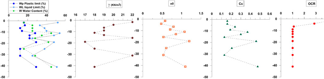
Figure 2. Soil parameters under the Sebou Embankment: W, water content; LL, liquid limit; PL, plastic limit; $\gamma$, unit weight; e0, initial ratio; Cc, coefficient of compressibility; OCR, over-consolidated ratio.

3.2 Finite element model and soil properties

For precise predictions, the Sebou Embankment subsoil is divided into 11 layers based on the parameter variation seen in Figure 2. Fifteen node triangular elements are used under plain strain conditions while using the very fine mesh option. The 2D plane-strain condition is used due to the soil layer symmetry in the N-S and E-W direction in the field, in addition to its light computation effort with quasi-similar results to the 3D model in this kind of boundary value geotechnical problems. The 2D model resulted in 1982 elements and 13,681 nodes (Figure 3).

Figure 3

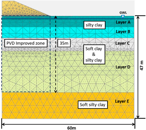
Figure 3. Geometry of the finite element model adopted for the simulation of the Sebou Embankment.

The water level is fixed at 2 m depth under the embankment base (while the updated mesh option is activated). Only half of the embankment is considered for symmetrical reasons. The model dimensions used are 60 m in the horizontal direction from the centerline of the full embankment and 47 m in the vertical direction. Lateral boundaries were restrained, and the drainage boundaries are considered to be at the piezometric level and at the bottom of the mesh.

The embankment is constructed from two filling materials: granular for the drainage layer in the embankment base and sandy material for the fill and the surcharge layers (see Figure 3). The Mohr–Coulomb model is selected for both materials, and the material parameters used are shown in Table 1.

Table 1

Table 1. Embankment parameter values.

$E^{\prime }$ is the Young modulus, $\nu$ is the Poisons ratio, and $\gamma$ is the unit weight of the embankment materials. The state variables and model constants for the embankment subsoil selected from laboratory tests (mainly oedometer test and direct shear test) for soft soil (SSM) and soft soil creep (SSCM) models are presented in Tables 2, 3.

Table 2

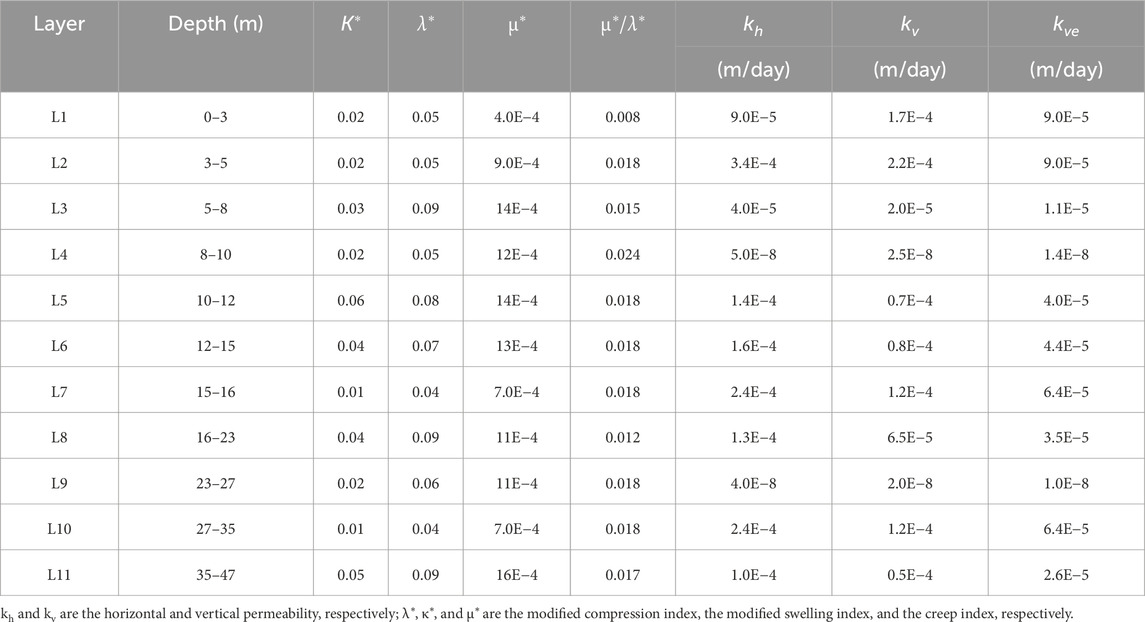
Table 2. Soil constant values for SSM and SSCM.

Table 3

Table 3. Initial parameters.

The lateral earth coefficient is calculated based on the equation $K_0=\left(1-\mathit{sin}{\phi }^{\prime }\right){OCR}^{\mathit{sin}{\phi }^{\prime }}$, and the permeability change index $C_k$ is calculated based on the equation $C_k=\frac{e-e_0}{\log \left(\frac{k}{k_0}\right)}$.

For Creep-SCLAY1S, the initial anisotropy (${\alpha }_0$) and its evolution uses soil constants $\omega$ (rate of surface rotation) and ${\omega }_d$ (rate of rotation due to deviator stress). The initial values of anisotropy and ${\omega }_d$ are derived theoretically based on the stress ratio at critical state M values for one-dimensional consolidation, the Equations 1–3 describing the above mentioned parameters are deduced based on Wheeler et al. (2003). The calculation methods are as follows.

${\alpha }_{k0}=\frac{{\eta }_{k_0}^2+3{\eta }_{k_0}-M_c^2}{3},(1)$

${\omega }_d=\frac{3}{8}\frac{4M_c^2-4{\eta }_{k_0}^2-3{\eta }_{k_0}}{{\eta }_{k_0}^2--M_c^2+2{\eta }_{k_0}},(2)$

${\eta }_{k_0}=\frac{3\left(1-K_0^{NC}\right)}{1+2K_0^{NC}}.(3)$

The parameter $\omega$ is calculated based on Equation 4 below:

$\omega =\frac{1}{{\lambda }^{*}}*\mathit{ln}\frac{10M^2-2{\alpha }_{k0}{\omega }_d}{M^2-2{\alpha }_{k0}{\omega }_d}.(4)$

Koskinen et al. (2002) suggested a procedure for determining the initial value of ${\chi }_0$, based on a fall cone test; the following Equation 5 is used:

${\chi }_0=S_t-1,(5)$

where $S_t$ is the sensitivity.

Krenn (2008) suggested both parameters $\xi$ and ${\xi }_d$ to have a good estimate for geomaterials of about $\xi =9$ and ${\xi }_d=0.2$

The values from the intrinsic compression index ${\lambda }_i$ and intrinsic creep parameter $\mu i\ast$ were carefully interpreted based on the assumption that $\raisebox{1ex}{$c^{\alpha }$}\!\left/ \!\raisebox{-1ex}{$\lambda $}\right.$ is a constant value for each layer, as mentioned by Mesri and Godlewski (1977). Values for $\mu i\ast$ , $\lambda i\ast$ , $k\ast$ were obtained from Equations 6–8 below:

${\mu }_i^{*}=c_{\alpha i}/{\mathit{ln}}_{10}\left(1+e_0\right),(6)$

${\lambda }_i^{*}={\lambda }_i/\left(1+e\right),(7)$

$k^{*}=k/\left(1+e\right),(8)$

where e is the void ratio. Table 5 summarizes the parameter values for each soil layer.

Table 5

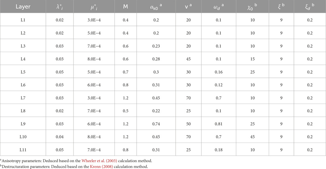
Table 5. Soil constant values for Creep-SCLAY1S.

3.3 Matching method

PVD installation influences soil stiffness and hydraulic conductivity of the surrounding soils. This impact and soil disturbance is difficult to assess, as different equipment is used by each soil improvement company (different mandrel types and dimensions). Hence, explicitly modeling drains and their smear zone area with highly estimated parameters can lead to discrepancies, in addition to high computational efforts and cost. Numerous methods can be adopted to calculate the equivalent permeability for the PVD-improved subsoil. In this paper, the matching approach described by Chai et al. (2001) is used in the matching process. This method uses the parameter of equivalent hydraulic conductivity ($k_{ve}$) for the PVD-improved zone without explicitly including the drain elements in the numerical model; the $k_{ve}$ is presented below as Equation 9:

${\mathrm{k}}_{\text{ve}}=\left(1+\frac{2.5{\mathrm{l}}^2{\mathrm{k}}_{\mathrm{h}}}{\mathrm{\mu }.{\mathrm{D}}_{\mathrm{e}}^2.{\mathrm{k}}_{\mathrm{v}}}\right).{\mathrm{k}}_{\mathrm{v}}.(9)$

l = drainage length, $D_e$ = diameter of a unit cell, and $k_h$, $k_v$ = horizontal and vertical hydraulic conductivity of subsoil. The parameter $\mathrm{\mu }$ is calculated by Equation 10:

$\mathrm{\mu }=\ln \left(\frac{\mathrm{n}}{\mathrm{s}}\right)+\frac{{\mathrm{k}}_{\mathrm{h}}}{{\mathrm{k}}_{\mathrm{s}}}\ln \left(\mathrm{s}\right)-\frac{3}{4}+\frac{2\mathrm{\pi }.{\mathrm{l}}^2.{\mathrm{k}}_{\mathrm{h}}}{3{\mathrm{q}}_{\mathrm{w}}},(10)$

where n = $D_e/d_w$ ($d_w$ = equivalent diameter of a PVD), s = $d_s/d_w$ and ($d_s$ is the equivalent diameter of the smear zone), $k_s$ = horizontal permeability of the smear zone, and $q_w$ = discharge capacity of a PVD. The adopted parameters related to the PVD-improved zone are given in Table 4.

Table 4

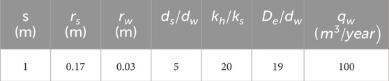
Table 4. Parameter values adopted for matching.

4 Sebou Embankment and field monitoring

Sebou Embankment is 4 m high and 14 m wide at the crest, with a footing of 38 m and 1:2 slope gradients. At first, a 0.3 m drainage layer was constructed from gravel, followed by a sandy filling material for the upper layers, including a 1.5 m thick preloading. As presented in Figure 4 the embankment construction timeline extended to over 3 years during the three main phases, fill construction, surcharge, and consolidation periods. All materials were compacted during the construction, attaining a density of 20 $\text{KN}/{\mathrm{m}}^3$. The embankment is constructed on improved subsoil with PVDs to meet the project specifications. In addition, to accelerate consolidation time, PVDs were installed in a rectangular pattern with 1 m spacing and a depth of 35 m. The embankment was monitored by field instrumentation that included settlement cells (SC), interstitial pressure sensors (IPS), and a piezometer (Figure 5).

Figure 4

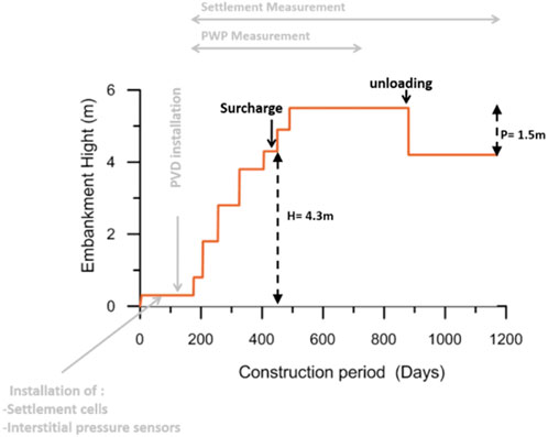
Figure 4. Embankment construction phases.

Figure 5

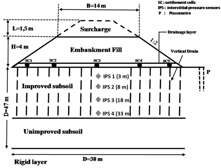
Figure 5. Cross section of the Sebou River Embankment.

Settlement cells were installed under embankment crests, slope toes, and the embankment centerline. The settlement measurements were taken based on a hydraulic comparison between the fixed settlement cell (reference settlement cell) and the settlement cells under the embankment. The measurements were taken with regular time intervals of approximately 3 days during the embankment construction, and the interval increased to one measurement each week during consolidation. Similarly, the pore pressure was measured in parallel with settlement measurements for the four interstitial pressure sensors. The measurement is done using a pressure gauge placed on the surface and connected to the probe by a tube filled with incompressible liquid. In addition, the water level was checked continuously.

5 Numerical modeling of PVD-improved ground

The calculated settlement based on standard constitutive models under the embankment at three locations, SC3, SC4, and SC5 (at the center, under the crest, and under the toe of the embankment, respectively) versus time is compared with the measured settlement and presented in Figure 6. As seen in Figure 6, there are some pronounced differences between the predicted settlement based on the soft soil model (SSM) versus the measured settlement. This is due to cumulative creep behavior that was captured when the soft soil creep model (SSCM) was included. As shown in Figure 6, during the embankment construction (between the 400-day mark and the end of settlement measurement), the SSM highly underestimated settlement versus when using SSCM (Figures 6A–C). Based on the comparison, the SSCM underestimated the settlement by an acceptable 12% under the embankment centerline and crest (Figures 6A, B) while underestimating the settlement by about 11% under the embankment toe. In contrast, the SSM underestimated the settlement with a significant 30% value compared to the measured settlement in all positions.

Figure 6

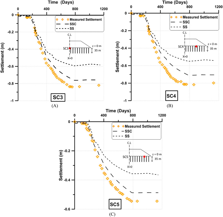
Figure 6. Time-settlement plot (A) at the center, (B) under the crest, and (C) at the Toe.

The settlement underestimation in the Sebou area, as presented by Mridakh et al. (2019), is due to the pronounced creep behavior in the alluvial deposits. For that, including a creep (time-dependent) component into the constitutive model is mandatory to tackle underestimated deformation, especially in the long term.

Figure 7 shows the predicted and the measured excess pore pressure (EPP) at a depth of 8 m. The predicted pore pressure based on SSM was larger than the measured one during the embankment construction phase (the first 400 days), which explains the main reason for good fit settlement immediately after the construction of the embankment, which is due to overestimation of the pore pressure build-up and dissipation rate when using SSM. The time-dependent model (SSCM) matched the measured EPP during the embankment construction. However, both SSM and SSCM underpredicted EPP during the consolidation process after the end of the embankment construction.

Figure 7

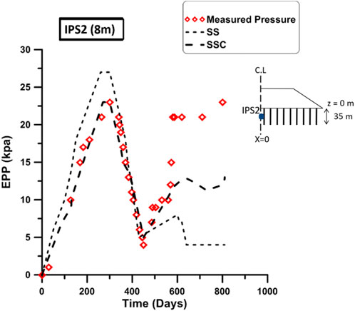
Figure 7. Excess pore pressure during construction at 8 m depth.

Based on the previous analysis, it is believed that Sebou alluvial deposits have an inherent time-dependent behavior that contributes to the EPP rate dissipation, especially in the long term. This inherent character can present some further deformation at a specific mean effective stress after the embankment construction. In addition, other mechanisms can be the cause for underestimating settlement and excess pore pressure.

Based on our interpretation, SSCM loses its advantage when used in over-consolidated soft soils by underpredicting the time-dependent behavior and underestimating the shear deformation for the first 3 m (L1), as presented in Figure 2 OCR. After a systematic evaluation of discrepancies in the predicted settlement and EPP, some points were raised and are summarized below:

• The permeability varies significantly between layers L3 and L4

• SSCM mostly predicts incorrect shear strains for a shear mobilization larger than $K_0^{NC}$-line for layers L1 and L2.

Based on these possible reasons for discrepancies, we pushed the numerical modeling analysis to explore a more advanced constitutive model, Creep-SCLAY1S.

Figure 8 shows settlement prediction versus time at SC3, SC4, and SC5; it is observed that settlement prediction by the Creep-SCLAY1S model matches well with the measured settlement. Although some higher rates of consolidation, as seen during the embankment construction period (first 400 days), can be due to the effect of stress concentration when using the critical state constitutive model, the model demonstrates a better capability of providing a precise simulation for higher number of layers with PVD treatment.

Figure 8

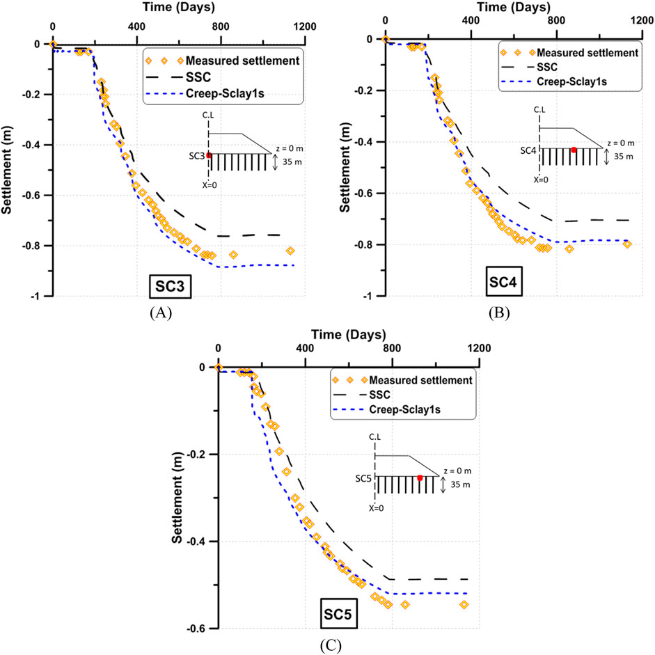
Figure 8. Time-settlement plot (A) at the center, (B) under the crest, and (C) at the Toe.

Due to the effect of stress concentration discussed previously, some slight variation in the predictions is seen in the long term (after the 400-day mark). Under the embankment centerline Figure 8A, a slight overestimation is observed of no more than 3% under the embankment crest (Figure 8B). In addition, the matching was nearly exact under the embankment toe (Figure 7C), and an underestimation of no more than 4% is measured.

Considering the plot of EPP prediction versus time in Figure 9, the predicted EPP when using the Creep-SCLAY1S model presented a rather high peak during the embankment construction (the first 400 days) while having an exact matching during the dissipation phase. After the construction phase, the Creep-SCLAY1S model presented a good match with the higher EPP measured in the field.

Figure 9

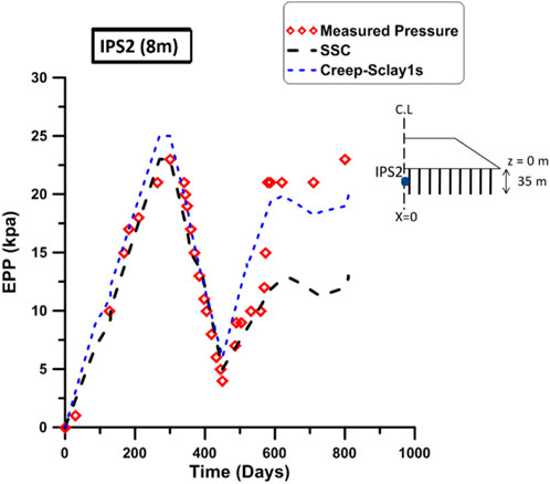
Figure 9. Excess pore pressure during construction at 8 m depth.

The Creep-SCLAY1S model showed a high-quality resemblance to the field behavior when including creep, destructuration, and fabric. Based on the results, both creep and destructuration mechanisms influenced the behavior of the Sebou deposits, especially in the long term. Those effects can only be captured simultaneously while including a constitutive model with a yield surface shape with a rotational component that can go higher than the $K_0^{NC}$-line and the failure M-line (Figure 1), especially when over-consolidated soft soil is present

6 Conclusion

This paper details the prediction procedure and data selection for prefabricated vertical drain (PVD) improved soft alluvial soils. A case study of the high-speed railway embankment in Sebou, Morocco, was analyzed numerically using two standard constitutive models, the soft soil model (SSM) and the soft soil creep model (SSCM), alongside an advanced model, Creep-SCLAY1S, to address the challenge of underestimating soil deformation in the naturally compressible soft alluvial deposits in the Sebou area. Based on the results, several conclusions were drawn:

✓ Incorporating creep and destructuration effects into the prediction process is crucial for accurate long-term behavior predictions in the Sebou area.

✓ The Creep-SCLAY1S model reasonably matches the measured behavior in Sebou.

✓ The time-independent soft soil model (SSM) is inadequate for predicting the delayed soil response in Sebou alluvial deposits.

✓ The soft soil creep model (SSCM) is suitable only for normally consolidated layers for settlement predictions in Sebou but does not accurately capture the delayed peak in excess pore pressure (EPP) after embankment construction.

✓ Although parameter selection for the Creep-SCLAY1S model is time-consuming, reliable methods and sensitivity analysis can lead to a better understanding of complex behaviors, which is beneficial for research and practical engineering applications

Data availability statement

The original contributions presented in the study are included in the article/supplementary material; further inquiries can be directed to the corresponding authors.

Author contributions

AM: conceptualization, methodology, validation, writing–original draft, and writing–review and editing. BN: conceptualization, investigation, methodology, validation, writing–original draft, and writing–review and editing. HE: investigation, validation, and writing–review and editing. HL: investigation, validation, and writing–review and editing.

Funding

The author(s) declare that no financial support was received for the research, authorship, and/or publication of this article.

Acknowledgments

The work presented was supported by the LPEE (Laboratoire Public d’Essais et d’Etudes). The first author would like to thank all personnel in the LPEE for providing all data necessary for the completion of this work.

Conflict of interest

The authors declare that the research was conducted in the absence of any commercial or financial relationships that could be construed as a potential conflict of interest.

Generative AI statement

The author(s) declare that no Generative AI was used in the creation of this manuscript.

Publisher’s note

All claims expressed in this article are solely those of the authors and do not necessarily represent those of their affiliated organizations, or those of the publisher, the editors and the reviewers. Any product that may be evaluated in this article, or claim that may be made by its manufacturer, is not guaranteed or endorsed by the publisher.

References

Amavasai, A., Sivasithamparam, N., Dijkstra, J., and Karstunen, M. (2018). Consistent class A and C predictions of the Ballina test embankment. Comput. Geotech. 93, 75–86. doi:10.1016/j.compgeo.2017.05.025

CrossRef Full Text | Google Scholar

Bagheri, M., and Rezania, M. (2021). Geological and geotechnical characteristics of London clay from the Isle of Sheppey. Geotechnical Geol. Eng. 39, 1701–1713. doi:10.1007/s10706-020-01572-3

CrossRef Full Text | Google Scholar

Chai, J. C., Shen, S. L., Miura, N., and Bergado, D. T. (2001). Simple method of modeling PVD-improved subsoil. J. Geotech. Geoenviron Eng. 127 (11), 965–972. doi:10.1061/(asce)1090-0241(2001)127:11(965)

CrossRef Full Text | Google Scholar

Cui, P., Fang, H., Wang, F., Cao, W., Zhang, X., Peng, B., et al. (2025). Nonlinear creep consolidation of vertical drain-improved soft ground with time-dependent permeable boundary under linearly construction load. Geotext. Geomembranes 53, 121–139. doi:10.1016/j.geotexmem.2024.09.001

CrossRef Full Text | Google Scholar

Guglielmi, S., Cotechia, F., Cafaro, F., and Gens, A. (2024). Analysis of the micro to macro response of clays to compression. Geotechnique 74 (2), 134–154. doi:10.1680/jgeot.21.00233

CrossRef Full Text | Google Scholar

Hashemi, H., Naeimifar, I., Uromeihy, A., and Yasrobi, S. (2015). Evaluation of rock nail wall performance in jointed rock using numerical method. Geotech. Geol. Eng. 33 (3), 593–607. doi:10.1007/s10706-015-9842-3

CrossRef Full Text | Google Scholar

Hosseinpour, I., Almeida, M. S. S., Riccio, M., and Baroni, M. (2017). Strength and compressibility characteristics of a soft clay subjected to ground treatment. Geotech. Geol. Eng. 35 (3), 1051–1066. doi:10.1007/s10706-017-0161-8

CrossRef Full Text | Google Scholar

Huang, J., and Griffiths, D. (2010). One-dimensional consolidation theories for layered soil and coupled and uncoupled solutions by the finite-element method. Géotechnique 60 (9), 709–713. doi:10.1680/geot.08.p.038

CrossRef Full Text | Google Scholar

Indraratna, B., Baral, P., Rujikiatkamjorn, C., and Perera, D. (2018). Class A and C predictions for Ballina trial embankment with vertical drains using standard test data from industry and large diameter test specimens. Comput. Geotech. 93, 232–246. doi:10.1016/j.compgeo.2017.06.013

CrossRef Full Text | Google Scholar

John, P. C. (2024). Constitutive modelling in computational geomechanics – 61st Rankine lecture, British Geotechnical Association, 2023. Géotechnique 74 (13), 1511–1535. doi:10.1680/jgeot.23.RL.001

CrossRef Full Text | Google Scholar

Karstunen, M., Krenn, H., Wheeler, S. J., Koskinen, M., and Zentar, R. (2005). Effect of anisotropy and destructuration on the behavior of murro test embankment. Int. J. Geomech. 5 (2), 87–97. doi:10.1061/(asce)1532-3641(2005)5:2(87)

CrossRef Full Text | Google Scholar

Kelly, R., Sloan, S., Pineda, J. A., Kouretzis, G., and Huang, J. (2018). Outcomes of the Newcastle symposium for the pre-diction of embankment behaviour on soft soil. Comput. Geotech. 93, 9–41. doi:10.1016/j.compgeo.2017.08.005

CrossRef Full Text | Google Scholar

Koskinen, M., Karstunen, M., and Wheeler, S. J. (2002). “Modeling destructuration and anisotropy of a natural soft clay,” in Proc.of the 5th European conf. Numerical methods in geotechnical engineering.

Google Scholar

Krenn, H. (2008). Numerical modelling of embankments on soft soils. Scotland: University of Strathclyde. Ph.D. thesis.

Google Scholar

Leoni, M., Karstunen, M., and Vermeer, P. A. (2008). Anisotropic creep model for soft soils. Geotechnique 58 (3), 215–226. doi:10.1680/geot.2008.58.3.215

CrossRef Full Text | Google Scholar

Mesri, G., and Godlewski, P. M. (1977). Time- and Stress Compressibility Interrelationship. J. Geotech. Engrg., ASCE 103 (5), 417–430.

CrossRef Full Text | Google Scholar

Mridakh, A. H., Ejjaaouani, H., Nguyen, B. P., Lahlou, F., and Labied, H. (2022). Soft soil behavior under high-speed railway embankment loading using numerical modelling. Geotech. Geol. Engrg. 40 (5), 2751–2767. doi:10.1007/s10706-022-02059-z

CrossRef Full Text | Google Scholar

Mridakh, A. H., Lahlou, F., Ejjaaouani, H., Mridekh, A., and Labied, H. (2019). Soil improvement of alluvial deposits under high-speed railway embankment: field case study. Geotech. Geol. Engrg. 37 (5), 3589–3603. doi:10.1007/s10706-019-00855-8

CrossRef Full Text | Google Scholar

Neher, H. P., Wehnert, M., and Bonnier, P. G. (2001). “An evaluation of soft soil models based on trial embankment,” in Proceedings of 10th international conference on computer methods and advances in geomechanics (Tucson), 373–378.

Google Scholar

NF P94-051 (1993). Sols: reconnaissance et essais- Détermination des limites d-atterberg – Limite de liquidité à la coupelle – Limite de plasticité au rouleau-Normes nationales et documents normatifs nationaux, 1–15.

Google Scholar

NF P94-071-1&2 (1993). Sols: reconnaissance et essais – Essai de cisaillement rectiligne à la boite – Partie 1: cisaillement direct – Normes nationales et documents normatifs nationaux, 1–16.

Google Scholar

NF P94-074 (1994). sols: reconnaissance et essais – Essai de cisaillement rectiligne à la boite – Partie 1/cisaillement direct – Normes nationales et documents normatifs nationaux, 1–36.

Google Scholar

Nguyen, B. P., Do, T. H., and Kim, Y. T. (2020). Large strain analysis of vertical drain-improved soft deposit consolidation considering smear zone, well resistance, and creep effects. Comput. qnd Geotech. 13c, 103602. doi:10.1016/j.compgeo.2020.103602

CrossRef Full Text | Google Scholar

Nguyen, B. P., Nguyen, T. T., and Mridakh, A. H. (2022a). Consolidation and load transfer characteristics of soft ground improved by combined PVD-SC column method considering finite discharge capacity of PVD’s. Indian geotech. J53, 127–138. doi:10.1007/s40098-022-00668-2

CrossRef Full Text | Google Scholar

Nguyen, B. P., Nguyen, T. T., Nguyen, T., and Guo, W. (2023). Analytical model for consolidation and bearing capacity of soft soil stabilized by combined PVD-deep cement mixing columns. Bull. Eng. Geo. Environ. J82, 286. doi:10.1007/s10064-023-03287-0

CrossRef Full Text | Google Scholar

Nguyen, B. P., Nguyen, T.-T., Nguyen, T. H. Y., and Tran, T.-D. (2022b). Performance of composite PVD–SC column foundation under embankment through plane-strain numerical analysis. Int. J. Geomechanics 22 (9), 04022155. doi:10.1061/(asce)gm.1943-5622.0002494

CrossRef Full Text | Google Scholar

Nguyen, T. T., and Indraratna, B. (2017). Experimental and numerical investigations into hydraulic behaviour of coir fibre drain. Can. Geotechnical J. 54 (1), 75–87. doi:10.1139/cgj-2016-0182

CrossRef Full Text | Google Scholar

Nguyen, T. T., and Indraratna, B. (2020). A coupled CFD–DEM approach to examine the hydraulic critical state of soil under increasing hydraulic gradient. ASCE-International J. Geomechanics 20 (9), 04020138. doi:10.1061/(asce)gm.1943-5622.0001782

CrossRef Full Text | Google Scholar

Nguyen, T. T., Indraratna, B., and Rujikiatkamjorn, C. (2018). A numerical approach to modelling biodegradable vertical drains. Environ. Geotech., 1–9. doi:10.1680/jenge.18.00015

CrossRef Full Text | Google Scholar

Rezania, M., Bagheri, M., Nezhad, M. M., and Sivasithamparam, N. (2017). Creep analysis of an earth embankment on soft soil deposit with and without PVD improvement. Geotext. Geomemb 45, 537–547. doi:10.1016/j.geotexmem.2017.07.004

CrossRef Full Text | Google Scholar

Silva, I. N., Indraratna, B., Nguyen, T. T., and Rujikiatkamjorn, C. (2024). The influence of soil fabric on the monotonic and cyclic shear behaviour of consolidated and compacted specimens. Can. Geotech. J. 61, 1159–1176. doi:10.1139/cgj-2023-0141

CrossRef Full Text | Google Scholar

Sivasithamparam, N., Karstunen, M., and Bonnier, P. (2015). Modelling creep behaviour of anisotropic soft soils. Comput. Geotech. 69, 46–57. doi:10.1016/j.compgeo.2015.04.015

CrossRef Full Text | Google Scholar

Taechakumthorn, C., and Rowe, R. K. (2012). Performance of a reinforced embankment on a sensitive Champlain clay deposit. Can. Geotech. J. 49, 917–927. doi:10.1139/t2012-053

CrossRef Full Text | Google Scholar

Vermeer, P. A., and Neher, H. P. (1999). “A soft soil model that accounts for creep,” in Beyound 2000 in computational geotechnics. Ten years of plaxis international balkema (Amsterdam), 249–261.

Google Scholar

Wheeler, S. J., Naatanen, A., Karstunen, M., and Lojander, M. (2003). An anisotropic elastoplastic model for soft clays. Can. Geotech. J. 40, 403–418. doi:10.1139/t02-119

CrossRef Full Text | Google Scholar

XP-94-090-1 (1997). sols: reconnaissance et essais – Essai oedométrique – Partie 1: essai de compressibilité sur matériaux fins quasi saturés avec chargement par paliers – Normes nationales et documents normatifs nationaux, 1–23.

Google Scholar

Yildiz, A. (2009). Numerical analyses of embankments on PVD improved soft clays. Adv. Eng. Softw. 40 (10), 1047–1055. doi:10.1016/j.advengsoft.2009.03.011

CrossRef Full Text | Google Scholar

Yildiz, A., Karstunen, M., and Krenn, H. (2009). Effect of anisotropy and destructuration on behavior of Haarajoki test embankment. Int. J. Geomechanics 9 (4), 153–168. doi:10.1061/(asce)1532-3641(2009)9:4(153)

CrossRef Full Text | Google Scholar

Glossary

${\mathit{\alpha }}_{\mathit{k}\mathbf{0}}$ initial value of anisotropy

${\mathit{\eta }}_{\mathit{k}\mathbf{0}}$ normally consolidated stress ratio

${\mathit{\chi }}_{\mathbf{0}}$ initial value of the bonding parameter

${\mathit{S}}_{\mathit{t}}$ sensitivity

$\mathit{\xi }$ parameter controlling the absolute rate of destructuration

${\mathit{\xi }}_{\mathit{d}}$ parameter controlling the relative effectiveness of destructuration rate

$\mathit{\omega }$ rate of rotation

${\mathit{\omega }}_{\mathit{d}}$ rate of rotation due to deviator stress

M stress ratio at critical state

${\mathit{M}}_{\mathit{c}}$ stress ratio at critical state in triaxial compression

${\mathit{\phi }}^{\prime }$ friction angle

${\mathit{c}}^{\prime }$ cohesion

e void ratio

${\mathit{e}}_{\mathbf{0}}$ initial void ratio

$\mathit{\gamma }$ unit weight

$\mathit{\nu }$ Poisson’s coefficient

${\mathit{k}}_{\mathbf{0}}$ coefficient of lateral earth pressure at rest

${\mathit{c}}_{\mathit{k}}$ permeability change index

${\mathit{c}}_{\mathit{\alpha }}$ creep index

${\mathit{c}}_{\mathit{\alpha }\mathit{i}}$ intrinsic creep index

k* modified slope of swelling/recompression line from the e _ lnp0 diagram

$\mathit{\lambda }$ slope of post-yield compression line from the e _ lnp0 diagram

${\mathit{\lambda }}_{\mathit{i}}$ slope of intrinsic post-yield compression line from the e-${lnp}_0$ diagram

${\mathit{\lambda }}^{*}$ Modified slope of post-yield compression line from the e-${lnp}_0$ diagram

${\mathit{\lambda }}_{\mathit{i}}^{*}$ Modified slope of intrinsic post-yield compression line from the e-${lnp}_0$ diagram

${\mathit{\mu }}^{*}$ modified creep index

${\mathit{\mu }}_{\mathit{i}}^{*}$ intrinsic modified creep index

NCS normal consolidation surface

$\mathit{\tau }$ reference time

k permeability

${\mathit{k}}_{\mathit{h}}$ horizontal permeability of undisturbed soil

${\mathit{k}}_{\mathit{h}\mathit{p}\mathit{l}}$ equivalent plane-strain horizontal permeability

${\mathit{k}}_{\mathit{s}}$ horizontal permeability of the smear zone

${\mathit{k}}_{\mathit{v}}$ vertical permeability of undisturbed soil

D equivalent diameter of unit cell

${\mathit{D}}_{\mathit{m}}$ equivalent diameter of mandrel

${\mathit{D}}_{\mathit{s}}$ equivalent diameter of the smear zone

${\mathit{D}}_{\mathit{w}}$ equivalent diameter of the drain

R equivalent radius of the unit cell

${\mathit{R}}_{\mathit{s}}$ equivalent radius of the smear zone

${\mathit{R}}_{\mathit{w}}$ equivalent radius of the drain

S drain spacing