Geometric characterization of locally corroded surfaces in steel bridge girders

The aging of steel bridge girders is often compounded by corrosion at girder ends due to leaking deck joints. With 6.8% of U.S. bridges in poor condition, there is an urgent need for accurate yet efficient methods to assess the residual load-bearing capacity of corroded girders. Traditional assessment methods often represent corrosion as uniform section loss or rely on simplified surface representations, compromising the accuracy of the residual capacity estimation. To address these limitations, this paper proposes a novel approach for characterizing the geometry of locally corroded steel surfaces by decomposing the corroded region into high-frequency (fine surface textures) and low-frequency (global shape) components using multilevel Lanczos filters. Validated using 3D scans collected from a 57-year-old in-service bridge, our case study shows that each high-frequency component can be modeled as a stationary random field using a Hole-Gaussian autocorrelation function, with correlation lengths inversely proportional to the cutoff frequencies of the Lanczos filters. The low-frequency component is accurately characterized by a bivariate Lagrange polynomial fitted via a 4 × 4 coefficient matrix, with average volume errors of less than 1% and normalized root mean square errors under 10% for most surfaces. The technique results in a manage set of parameters that can be used to investigate the effects of corrosion damage on the behavior of corroded steel members.

1 Introduction

The aging of steel bridge girders, often accelerated by corrosion at girder ends due to leaking deck joints, poses significant safety concerns and maintenance challenges (Kayser and Nowak, 1989; Kere and Huang, 2019). As a result, repair has become an increasingly crucial aspect of bridge engineering (Alemdar et al., 2014; Zmetra et al., 2017; McMullen and Zaghi, 2020). According to a recent report by the ASCE (2025), 45% of bridges in the United States have exceeded their 50-year design life and 6.8% of all bridges are in poor condition. Despite increased government investment, funding remains insufficient to perform all necessary repairs (ASCE, 2025). Given these constraints, assessing the impact of corrosion damage on the residual load-bearing capacity of steel bridge girders is essential to effectively prioritize future rehabilitation projects.

Numerous studies have investigated the impact of corrosion-induced section loss on bridge girders (Liu et al., 2011; Tohidi and Sharifi, 2016). For example, Tzortzinis et al. (2021b) conducted numerical studies on corroded girders from decommissioned bridges and developed closed-form equations to estimate their residual capacity using parameters such as the average web thickness. However, the accuracy of these investigations is limited by challenges in modeling corrosion damage, including the difficulty of obtaining detailed data and accounting for the irregular geometry of the remaining steel surfaces. Traditional inspection methods measure corrosion depths at only a few discrete locations, providing insufficient data to accurately estimate a corroded girder’s residual capacity. Conversely, highly detailed representations require thousands of data points to capture the corroded surface’s intricate geometry (Qin et al., 2016; Zhang and Zaghi, 2023). Incorporating such detail into analysis is computationally prohibitive due to the need for large data structures and significant processing power (Tzortzinis et al., 2022). Thus, there is a critical need for methods to distill high-dimensional representations of corrosion damage into manageable parameter sets.

Characterizing the geometry of corrosion damage offers one approach to address these challenges. Rather than relying on a detailed corrosion depth map, geometric characterization represents the damage using a small set of key parameters. Past studies have extracted various characteristics from corrosion damage to facilitate girder capacity evaluations (Appuhamy et al., 2011; Sharifi and Tohidi, 2014; Tohidi and Sharifi, 2016; Tzortzinis et al., 2021a). For example, Khurram et al. (2014a) and Khurram et al. (2014b) proposed the use of corrosion damage height, depth, and a reduced thickness ratio to characterize the damage. In another study, Bao et al. (2021) described corrosion damage using a uniform section loss parameter, reducing the thickness of the web. Kanakamedala et al. (2023) also modeled corrosion damage using an effective web thickness. In their study, the effective thickness was applied to a trapezoidal region of the beam defined by the length and height of the corroded area. Although these methods have improved analysis outcomes, they make significant simplifications and fail to account for the intricate geometry of the corroded surface. Such simplifications can be problematic as corrosion can lead to stress concentrations (Shojai et al., 2022) that cause significant errors in residual capacity estimates (Prucz and Kulicki, 1998; Mokhtari and Melchers, 2018). In some cases, up to 100% error can be present in the final estimate (Hain et al., 2021; Tzortzinis et al., 2021a). To overcome these limitations, this study develops a novel characterization method to decompose the nuanced geometry of a corroded steel surface into information-rich parameters, moving beyond the use of simple geometric parameters like average corrosion depth.

In addition to geometric parameters, many researchers have used statistical models to characterize corroded surfaces (Teixeira and Soares, 2008; Melchers et al., 2010; Deliang et al., 2021). For instance, Htun et al. (2013) used random fields to model the surface geometry of a uniformly corroded plate on a ship, using statistical features such as mean, variance, and correlation length. Their analysis demonstrated that a random field can accurately model a corroded surface when the correlation length is less than one-third of the plate size. However, this approach is limited to uniform corrosion damage because it assumes the corroded surface to be a stationary random field. In the case of a uniformly corroded surface, the mean and variance calculated from the entire surface can be used to characterize the entire surface. Unlike uniformly corroded surfaces, the textures of locally corroded members vary by location. For example, corrosion depth is not uniform. Because of this, the topology of a locally corroded surface is defined by multiple waves with different wavelengths that cannot be accurately represented by a single set of statistical parameters (Leach, 2013).

Kriging is a classic geostatistical method for spatial modeling and random field prediction that estimates values at unsampled locations based on autocorrelation and observed values (van Beers and Kleijnen, 2003; Bagtzoglou and Hossain, 2009; Kleijnen, 2009). Universal kriging, which models the overall shape and variation—the two fundamental components of a locally corroded surface—as the sum of a trend function and a random field (Zimmerman et al., 1999), cannot adequately model the multiple scales of texture present on locally corroded surfaces because only the component with the largest variation is captured. To address this limitation, our study uses Lanczos filters (Duchon, 1979) to decompose the true geometry of a locally corroded surface into several high-frequency components, each corresponding to a distinct random fields.

Note that characterizing a corroded surface requires a model of the existing corrosion damage. Researchers have proposed various approaches to develop these models, including the use of cellular automata models and 3D scanning. While cellular automata models can be used to generate artificial corroded surfaces (Pérez-Brokate et al., 2016; Zhu et al., 2018; Stępień et al., 2019), they cannot be used to model real corroded surfaces. In contrast, 3D scanning technology captures the complex geometry of real corroded surfaces with high precision (Hain et al., 2019; Tzortzinis et al., 2022). Accordingly, this study leverages 3D scanning to advance the novel image processing technique for the characterization of a corroded surface.

Image processing has proven to be a crucial tool. As a recent review by Salunkhe et al. (2022) has shown, image processing has been widely applied in civil engineering to both the repair and maintenance of structures. For example, some researchers have developed corrosion detection algorithms using unmanned aerial vehicles (Das et al., 2023), while others have developed neural network-based classifiers of corrosion damage and corrosion intensity (Forkan et al., 2022; Munawar et al., 2022). These image processing methods, however, fail to provide formal assessments of capacity loss. To overcome this, researchers have developed finite element models of corroded members from 3D scans. While these models have proven to be accurate (Sun et al., 2025), the method becomes computationally prohibitive as the size of the corroded region increases. This has led researchers to develop global characterizations, using parameters like percent mass loss, to investigate corrosion’s impact on a material’s nominal properties (Yan et al., 2024). As noted earlier, though, these parameters do not account for the unique surface geometry of the corroded region.

To address these challenges, the technique developed in Section 2 decomposes a locally corroded surface into multilevel high-frequency components and a single low-frequency component that represent the different scales of textures and the overall shape of the corroded surface, respectively. By decomposing the corroded surface into multiple components, the original surface can be characterized on multiple levels. This results in a richer characterization than would result from simple geometric or otherwise universal parameters that can be used to inform future bearing capacity evaluations. The high-frequency components are characterized using statistics describing the distribution of height values and the autocorrelation function (ACF) since they can be considered stationary random fields. The low-frequency component is characterized via a polynomial function that preserves the overall shape of the corroded surface (Weiss et al., 2002; Nurunnabi et al., 2014).

2 Methodology

This section proposes a comprehensive geometric characterization method for corrosion damage at the ends of steel girders. The geometry of a locally corroded surface comprises two main components: the fine textures of the remaining steel (high-frequency components) and the underlying shape of the corroded region (low-frequency component). We decompose the corroded surface into these components using Lanczos filters. These filters ensure a consistent and predictable decomposition across different corroded surfaces when compared with other approaches such as wavelets, which require careful selection of the mother wavelet and extensive parameter tuning (Guo et al., 2022).

We use different methods to characterize the high- and low-frequency components due to their distinct properties. For the high-frequency components, the statistical distribution of corrosion depth values and the ACF are used. For the low-frequency component, a bivariate polynomial function is used. Together, the properties of the high- and low-frequency components yield a numerically concise yet substantial set of parameters that describe the original corroded surface.

2.1 Decomposing the locally corroded surface into high- and low-frequency components

To facilitate the decomposition, the corroded surface is represented using a corrosion depth map. Figure 1a shows an example of a locally corroded surface obtained from a 3D scan of an in-service steel bridge girder. The extent of corrosion damage is indicated by the color intensity, with darker colors representing greater corrosion depths. Figure 1b displays the same corroded surface as a 2D corrosion depth map, represented mathematically as a matrix.

Figure 1

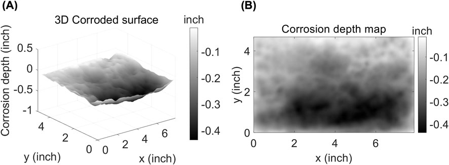
Figure 1. A typical locally corroded surface obtained from a 3D scan of an in-service steel-girder bridge. (A) 3D representation of the corroded surface, and (B) the corresponding 2D corrosion depth map.

The locally corroded surface is first decomposed into multilevel high-frequency components and one low-frequency component. Generally, there are two ways to decompose a surface into high-frequency and low-frequency components. The first is the surface-fitting method in which a function with unknown parameters is proposed to fit the surface. Here, the parameter values are determined using the least squares method based on sample points on the surface (Weiss et al., 2002; Nurunnabi et al., 2014). The resulting function is the low-frequency component, while the high-frequency component is obtained by subtracting the low-frequency component from the original surface. This method is typically used when the shape of the surface can be represented using a simple, closed-form expression. The other technique is the surface-filtering method in which a filter with a defined cutoff frequency is applied to the surface. The latter method is used in this research for two reasons. First, by defining the same cutoff frequency, the high-frequency and low-frequency components for different corroded surfaces will be separated at the same frequency, ensuring consistency in the decomposition and subsequent characterization. Second, the surface-fitting method cannot extract multilevel high-frequency components. By using multiple filters with different cutoff frequencies in the surface-filtering method, the high-frequency components can be decomposed into multiple levels.

Lanczos filters are used in this study to decompose the locally corroded surfaces as they can be easily constructed and are able to accurately separate low-frequency and high-frequency components. The Lanczos filter is a low-pass filter created by multiplying a sinc function, shown in Equation 1 and plotted in Figure 2a, by a window function. The sinc function is a symmetrical decayed sine wave and is the impulse response of an idealized low-pass filter, as demonstrated by the rectangular frequency response shown in Figure 2b (Woodward and Davies, 1952). Convolution of a surface with this filter ideally removes the components above the cutoff frequency without affecting the low-frequency components. Due to its infinite length in the spatial domain, the sinc filter is not physically realizable. Thus, a scaled sinc window is applied to the sinc function to limit the length of the filter. The result is a Lanczos filter, shown in Equation 2 (Lanczos, 1988). The parameter k is a positive integer that determines the filter size. The larger the parameter k, the closer the performance of the Lanczos filter is to the ideal sinc filter, but the higher the computational complexity. The most common values for k are 2 or 3.

$\text{sinc}\left(x\right)=\left\{\begin{array}{ll}\frac{\sin \left(\pi x\right)}{\pi x}& x\ne 0\\ 1& x=0\end{array}\right.(1)$

$\text{Lanczos}\left(x\right)=\left\{\begin{array}{ll}\text{sinc}\left(x\right)\text{sinc}\left(\frac{x}{k}\right)& -k<x<k\\ 0& \text{otherwise}\end{array}\right.(2)$

Figure 2

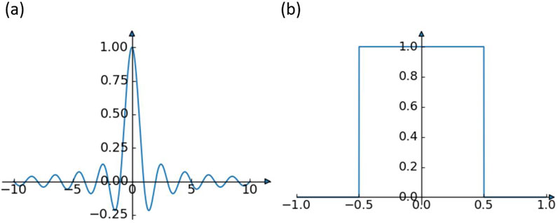
Figure 2. Sinc function and its frequency response. (a) Sinc function in the spatial domain between −10 and 10, and (b) Frequency response of the sinc function.

The proposed method constructs a series of 2D Lanczos filters with the parameter k = 3 (hereon referred to as Lanczos3 filters) to decompose a locally corroded surface. The Lanczos3 filters have larger roll off rates than Lanczos2 filters (k = 2), resulting in a clearer separation of the frequency components. Further, Lanczos3 filters provide a reasonable balance between filter size and computational complexity. Increasing the value of k further has limited impact on the results while increasing the computational complexity. To adjust the filter’s cutoff frequency, we substitute the x in Equation 2 with x/2^l (where l = 1, 2, 3 …), as shown in Equation 3. Each increment in l halves the cutoff frequency and doubles the filter size. Next, the filters are discretized by computing the values of the filter at all integers between −3 × 2^l and 3 × 2^l. For each level l, the discretized filter is a vector v_l of length 3 × 2^l+1-1. For instance, when l is equal to 1, 2, and 3, the corresponding vector lengths are 11, 23, and 47, respectively. The vectors of the discretized Lanczos3 filters are then normalized such that the elements in each vector v_l sum to 1, ensuring that the passed low-frequency component has the same mean value as the original surface. Figure 3 illustrates the normalized Lanczos3 filter and the corresponding frequency response for l = 1 and l = 2. By comparing Figure 3a with Figure 3c, it can be seen that when l increases from 1 to 2, the domain of the Lanczos3 function changes from [−6, 6] to [−12, 12]. In total, 11 discretized points ranging from −5 to 5 are obtained from the Lanczos3 function with l = 1. Note that the zeros at −6 and 6 are not included. Due to the limited ranges of these Lanczos filters, the corresponding frequency responses (Figures 3b, d) exhibit roll-off between the passband and the stopband. However, the shape of the Lanczos filter’s frequency response is similar to that of the sinc filter, with roll-off occurring around the cutoff of the sinc filter (see Figures 3b, d). Therefore, the cutoff frequencies of the Lanczos3 filters are approximated as those of the corresponding sinc filters, which are 0.5/2^l. Finally, the 2D Lanczos3 filters are constructed. A 2D discrete Lanczos3 filter is created as the outer product of the normalized vector v_l with itself, yielding a (3 × 2^l+1−1) × (3 × 2^l+1−1) matrix.

$\text{Lanczos}3\left(x,l\right)=\left\{\begin{array}{ll}\text{sinc}\left(\frac{x}{2^l}\right)\text{sinc}\left(\frac{x}{3\left(2^l\right)}\right)& -3\left(2^l\right)<x<3\left(2^l\right)\\ 0& \text{otherwise}\end{array}\right.l=1,2,3,\dots (3)$

Figure 3

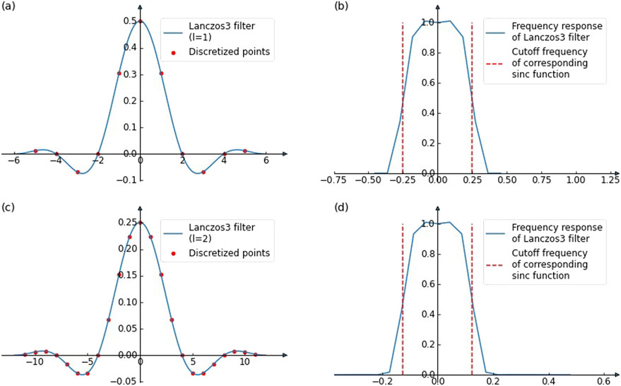
Figure 3. Normalized Lanczos3 filter and the corresponding frequency response for l = 1 and 2. (a, b) are the Normalized Lanczos3 filter for l = 1 and its frequency response, (c, d) are the Normalized Lanczos3 filter for l = 2 and its frequency response.

Once the 2D Lanczos3 filters are constructed, the locally corroded surface is decomposed into multilevel high-frequency components and one low-frequency component following the procedure shown in Figure 4. The first step is to convolve the corroded surface with the first Lanczos3 filter (l = 1 in Equation 3). Because the Lanczos filters are low-pass filters, the resulting surface includes the components with frequencies lower than the cutoff frequency. For the first Lanczos3 filter, this is 0.5/2¹, or 0.25. The first high-frequency component is then obtained by subtracting the filtered surface from the original corroded surface. These two steps are then repeated using Lanczos3 filters with increasing values of l to extract subsequent high-frequency components. The wavelengths of the extracted high-frequency components increase with the levels (l) of the Lanczos filters. The process is repeated until the wavelength is comparable to the size of the corroded surface. The last remaining filtered surface is taken as the low-frequency component.

Figure 4

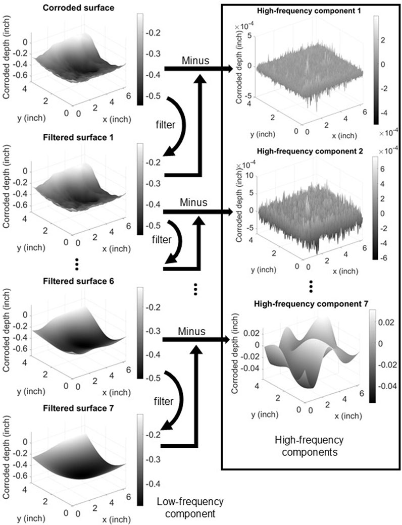
Figure 4. Decomposing a locally corroded surface into multilevel high-frequency components and one low-frequency component.

The convolution process produces an output surface of size M-N+1, in which M is the length (or width) of the original image in pixels and N is the corresponding side length of the filter. Because the convolution process reduces the image size, we use padding (Strang and Nguyen, 1996) to preserve the original dimensions. Specifically, antisymmetric padding is used in this study since it ensures that the padded surface and its derivative are continuous at the boundary, minimizing the boundary errors in the filtered surface. Therefore, the original corroded surface can be fully reconstructed by summing all frequency components.

2.2 Characterizing the high-frequency components

Each high-frequency component is considered a stationary, isotropic 2D random field. Two random field features are computed to characterize each component: the statistical distribution of height values and the ACF. The distribution of height values characterizes the magnitude of the waves in each high-frequency component, describing its out-of-plane dimension, while the ACF characterizes the wavelength of the waves in each high-frequency component, describing its in-plane dimension.

2.2.1 Statistical distribution of height values

The distribution of height values is investigated by plotting the histogram of height values for each high-frequency component and comparing the shapes of the histograms with the normal distribution. While mean and standard deviation are both commonly used to characterize random fields, all high-frequency components have theoretical means of zero (see Figure 4). Therefore, the proposed method uses the standard deviation only to characterize each high-frequency component. Section 3.2.1 demonstrates this process using a case study.

2.2.2 Autocorrelation function

The ACF is commonly used to characterize how points in a random field are correlated (Lin et al., 1997). In physical applications, such as modeling a corroded surface, the field’s height values are usually continuous. As a result, two points that are close together tend to be highly correlated. This correlation diminishes as the distance between the two points grows. The ACF quantifies the rate at which these correlations decay with increasing distance. In this study, the ACF is used to characterize the spatial dependence of the height values in the high-frequency components, which is crucial for subsequent analysis and modeling of corroded surfaces.

Because the high-frequency components are considered stationary and isotropic, the correlation between any two points depends solely on the distance between them (Htun et al., 2013). The ACF, shown in Equation 4, is the expected autocorrelation value of two points as a function of the distance d between them. Here, x₁ and x₂ are two points in a random field, Y(x₁) and Y(x₂) are the height values at points x₁ and x₂, and μ and σ denote the mean and standard deviation of all height values in the random field, respectively. Although the theoretical mean values of the high-frequency components are zero, the actual means may not be due to the limited size of the corroded surface.

$\rho \left(d\right)=\frac{E\left[\left(Y\left({\mathit{x}}_1\right)-\mu \right)\left(Y\left({\mathit{x}}_2\right)-\mu \right)\right]}{{\sigma }^2}(4)$

The shape of the ACF can vary widely for different random fields. Researchers have proposed various autocorrelation models using different functions, such as exponential, linear-exponential, Gaussian, and spherical (Ababou et al., 1994). Each autocorrelation model has a distance-related parameter termed the correlation length (l_c), which can be calculated by fitting the corresponding function to the ACF. In this study, the Hole-Gaussian ACF is used (Ababou et al., 1994).

2.3 Characterizing the low-frequency component

The low-frequency component represents the underlying shape of the corroded surface. A bivariate polynomial function is chosen to characterize the low-frequency component since these components are generally smooth surfaces and a bivariate polynomial can be fit to a smooth surface with high accuracy. In this way, a low-frequency component initially represented as a matrix with many elements can be characterized using a small number of polynomial coefficients. In addition, surface features can be easily obtained from the polynomial function. For instance, the slope and curvature of a surface can be obtained by calculating its derivatives.

Two primary methods exist for constructing a bivariate polynomial, z = f(x, y), from a surface using a set of sample points: fitting and interpolation. The fitting method aims to find a polynomial surface that is overall the closest to the sample points without necessarily passing through them using the least-squares method. Typically, a much larger number of sample points is used compared to the polynomial’s degree and a bivariate polynomial with unknown coefficients is assumed. On the other hand, interpolation ensures that the generated surface passes through all sample points. This method is more computationally efficient because there is no need to compute the matrix inverse. In 2D cases, given a grid-pattern sample-point set with m + 1 columns in the x direction and n + 1 rows in the y direction, a unique polynomial with a degree of m for x and n for y can be found. In this study, the Lagrange interpolation method is used as it provides an efficient way to identify the unique polynomial (Werner, 1984). In addition, the Lagrange polynomial is comparably accurate to the least-squares method when the surface is smooth, as is true for the low-frequency components.

Assuming the sample-point set can be represented as (x_i, y_j, z_i,j), i = 0, 1, 2, …, m; j = 0, 1, 2, …, n, the Lagrange basis corresponding to the sample point (x_i, y_j, z_i,j) can be constructed (Equation 5). This basis has the following properties: (1) l_i,j (x_p, y_q) = 0 if p ≠ i or q ≠ j, (2) l_i,j (x_i, y_j) = 1, and (3) l_i,j (x, y) has a degree of x as m and a degree of y as n. The Lagrange polynomial representing the surface can be constructed as a linear combination of the bases with weights equal to the corresponding z values, as shown in Equation 6.

$l_{i,j}\left(x,y\right)={\prod }_{\begin{array}{c}0\le p\le m\\ p\ne i\end{array}}\frac{x-x_p}{x_i-x_p}{\prod }_{\begin{array}{c}0\le q\le n\\ q\ne j\end{array}}\frac{y-y_q}{y_j-y_q}\left(0\le i\le m,0\le j\le n\right)(5)$

$f\left(x,y\right)={\displaystyle \sum _{0\le i\le m,0\le j\le n}}{z}_{i,j}{l}_{i,j}\left(x,y\right)(6)$

We construct the Lagrange polynomial from a grid of sample points. Two sampling methods are compared: n-section points sampling and Gauss points sampling (Swarztrauber, 2003). Figure 5 demonstrates 4 × 4 sampling using these two different methods. In the n-section points sampling, shown in Figure 5a, the rectangle has a size of a × b and the origin is at the lower left. The positions of the sample points in the x and y directions are the trisection points of the edges, i.e., 0, 1/3, 2/3, and 1. For the Gauss points sampling in Figure 5b the plate size is, by convention, defined as 2a × 2b and the origin is at the middle of the rectangle. The positions of the sample points in both directions are the four-point case Gauss points, i.e., −0.86, −0.34, 0.34, and 0.86.

Figure 5

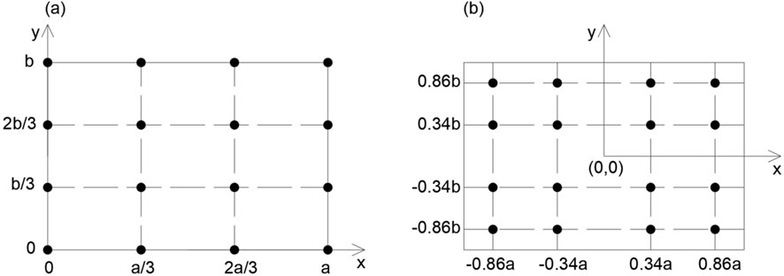
Figure 5. The 4 × 4 sampling points using different methods – (a) n-section points sampling and (b) Gauss points sampling.

After determining the polynomial for the low-frequency component, the approximated surface can be constructed by calculating the z value at any position on the fitted surface based on its coordinates (x, y), as shown in Equation 7. The n × m coefficient matrix A governs the approximated surface. Representing the low-frequency component as a bivariate Lagrange polynomial simplifies the characterization of a matrix with thousands of elements (corresponding to a single low-frequency component) into an n × m coefficient matrix in which a_ij is the coefficient of the polynomial term x^jyⁱ.

$z={\mathit{y}}^{\mathrm{T}}\mathit{A}\mathit{x}={\left[\begin{array}{c}1\\ ⋮\\ y^n\end{array}\right]}^{\mathrm{T}}\left[\begin{array}{ccc}{a}_{00}& \cdots & a_{0m}\\ ⋮& \ddots & ⋮\\ a_{n0}& \cdots & a_{nm}\end{array}\right]\left[\begin{array}{c}1\\ ⋮\\ x^m\end{array}\right](7)$

The three steps discussed above decompose a locally corroded surface into high-frequency and low-frequency components and characterize them individually. The high-frequency components are characterized using the statistical distribution of the height values and the ACF, while the low-frequency component is characterized using a bivariate Lagrange polynomial function. Section 3 will demonstrate the application of the proposed methodology with a case study.

3 Case study

The proposed methodology is applied to and validated using five locally corroded surfaces obtained from 3D scans of steel girders from a 57-year-old in-service bridge. The five surfaces were measured using an Artec Eva 3D scanner, which has a resolution of 0.5 mm and an accuracy of 0.1 mm (Artec3D, 2019). The five surfaces are shown in Figures 6a–e. Surface 3 results from a scan of a corroded stiffener plate, while the remaining four surfaces are from scans of corroded web plates. The dimensions of the five corroded surfaces are as follows: 7.9 inches (200 mm) × 4.7 inches (119 mm), 7.4 inches (188 mm) × 3.4 inches (86 mm), 6.9 inches (175 mm) × 6.3 inches (160 mm), 7.8 inches (198 mm) × 4.8 inches (122 mm), and 6.4 inches (163 mm) × 3.9 inches (99 mm), respectively. Maximum corrosion depths of the five surfaces range from 0.2 to 0.5 inches (5–12.7 mm). The pixel size for all five corroded surfaces is 0.02 inches (0.5 mm). To evaluate the consistency of the characterization technique proposed above, we compare characteristics such as the height value standard deviation and the correlation length for the high-frequency components of these five corroded surfaces.

Figure 6

Figure 6. The corrosion depth maps (inches) of five locally corroded surfaces from real bridge girders – (a–e): corroded surfaces 1 to 5, respectively.

3.1 Decomposing the locally corroded surface

Each of the five corrosion depth maps is decomposed into seven high-frequency components and one low-frequency component following the procedure described in Section 2.1. As an example, Figure 7 illustrates the decomposition of corroded surface 1 from Figure 6a. Based on Section 2.1, the cutoff frequencies of the Lanczos3 filters are (0.5/2^l)/L, where L represents the pixel size (0.02 inch). The cutoff frequencies for the seven filters are 12.5 in⁻¹, 6.25 in⁻¹, 3.125 in⁻¹, 1.563 in⁻¹, 0.781 in⁻¹, 0.391 in⁻¹, and 0.195 in⁻¹, respectively. The last high-frequency component has a wavelength of approximately 5.1 inches, which is comparable to the dimensions of the corroded surfaces shown above in Figure 6. Therefore, further extraction of high-frequency components (Figures 7a–g) is not required, and the remaining surface is the low frequency component (Figure 7h).

Figure 7

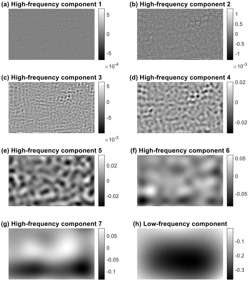
Figure 7. The high-frequency and low-frequency components of corroded surface 1 – (a–g): Seven high-frequency components, and (h): One low-frequency component.

3.2 Characterizing the high-frequency components

As discussed in Section 2.2, two random field features—the statistical distribution of height values and the ACF—are calculated to characterize each of the high-frequency components.

3.2.1 Statistical distribution of height values

Figure 8 displays histograms of height values for each of the high-frequency components from corroded surface 1 (Figure 6a). We compute the mean and standard deviation for each component to assess their distribution. It is observed that the standard deviation of height values increases with the level of the high-frequency component and that all mean height values are much less than the corresponding standard deviations. This is expected since the theoretical mean of the high-frequency components is zero. The small non-zero mean values are attributed to the errors caused by the limited sizes of the corroded surfaces. The histograms are compared qualitatively to the probability density function of a normal distribution with the same mean and standard deviation. This normal distribution is plotted in red in Figure 8 for each component. It is observed that the distributions of the height values in high-frequency components 1 to 5 are very close to the normal distribution. For high-frequency components 6 and 7, the discrepancy between the histograms and the normal distribution can be attributed to the limited fluctuation of waves captured in the corroded region. The distributions of the height values have similar ranges and trends for all five corroded surfaces.

Figure 8

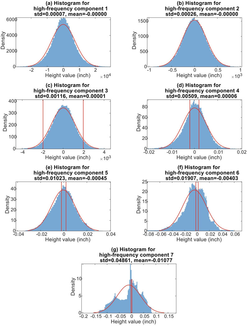
Figure 8. (a–g) Histograms of the height values in high-frequency components 1 to 7, respectively, of corroded surface 1.

Before a more detailed investigation of the statistical distribution, it is first necessary to verify the accuracy of the extracted high-frequency components. Two vertical red lines are drawn at +/−0.05 mm (+/−1.97 × 10⁻³ inch) in each histogram in Figure 8. These lines correspond to the positive and negative half of the scanner’s accuracy. Data between these lines represent fluctuations in corrosion depth that are smaller than the scanner’s accuracy. These two lines are not displayed for high-frequency components 1 and 2 since all height values are in ranges smaller than the scanner’s accuracy. This is also true for most data in the third high-frequency component. As such, the accuracy of high-frequency components 1, 2, and 3 cannot be guaranteed. The following discussion therefore focuses on high-frequency components 4 to 7 for all five locally corroded surfaces. As shown by Figure 9, excluding these three high-frequency components does not lead to significant errors between the reconstructed and as-scanned surfaces. We further note that 0.1 mm is a relatively high accuracy for investigating corrosion on steel bridge girders. When compared to typical plate member thicknesses, which range from 0.375 inches (9.5 mm) to more than 2 inches (50.8 mm), the error is around 0.2%–1%, which is acceptable.

Figure 9

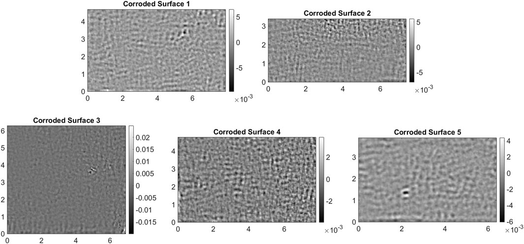
Figure 9. Error between the scanned corroded surface and the reconstructed surface excluding high-frequency components 1, 2, and 3 (inches). These three frequency components are left out of the analysis as they primarily correspond to noise.

The relationship between the standard deviation of height values and the cutoff frequency of the Lanczos3 filter used for decomposition is used to quantitatively characterize the high-frequency components. The standard deviations of the height values in high-frequency components 4 to 7 and the corresponding cutoff frequencies of the Lanczos3 filters are listed in Table 1. The average value of the standard deviations for each high-frequency component is calculated across the five surfaces. For every increase in the high-frequency component level, the cutoff frequency halves while the average standard deviation of height values approximately doubles. A reciprocal function y = b/x is proposed to fit the standard deviation as a function of the cutoff frequency. The parameter b is obtained using the least-squares method as 6.297 × 10⁻³. All the standard deviation values and the fitted curve y = 6.297 × 10⁻³/x (solid curve) are plotted in Figure 10a. The curve fits the trend of the standard deviations well; however, the standard deviations for each cutoff frequency still show some variation due to the varying corrosion intensities. The coefficient of variation (CV) of the standard deviations is used to quantify this variation. The CV of the standard deviation values for each level of high-frequency component is listed in Table 1, ranging from 0.176 to 0.356. The average of all CV values is 0.264, which quantifies the overall variation of the standard deviation values. The two dashed black curves drawn in Figure 10a correspond to this CV and show the variation in the standard deviations of height values across the five corroded surfaces.

Table 1

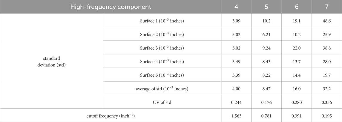
Table 1. The standard deviation of the height values in the high-frequency components for all five corroded surfaces and corresponding cutoff frequencies.

Figure 10

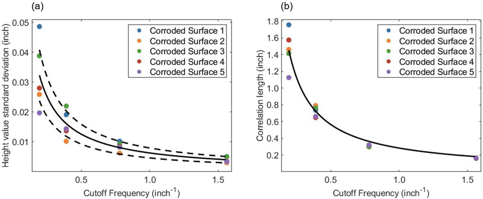
Figure 10. (a) Standard deviations of height values in high-frequency components of the corroded surfaces vs. the cutoff frequency of Lanczos3 filters. (b) The fitted function for correlation lengths of the high-frequency components against the cutoff frequency of the Lanczos3 filter.

3.2.2 Autocorrelation function

The ACF is calculated for each high-frequency component using Equation 4. The resulting ACFs are plotted in blue for corroded surface 1 in Figure 11. As expected, the autocorrelation value is 1 when the distance between the two points is 0. As the distance increases, the autocorrelation decreases and approaches 0. From a comparison of the ACFs with the most common autocorrelation models, the Hole-Gaussian ACF (Ababou et al., 1994) is adopted. The Hole-Gaussian function is depicted in Equation 8 as a function of the distance d between points, where l_c refers to the correlation length for the Hole-Gaussian autocorrelation model.

$S\left(d\right)=\left(1-{\left(\frac{d}{l_c}\right)}^2\right)\exp \left(-\frac{1}{2}{\left(\frac{d}{l_c}\right)}^2\right)(8)$

Figure 11

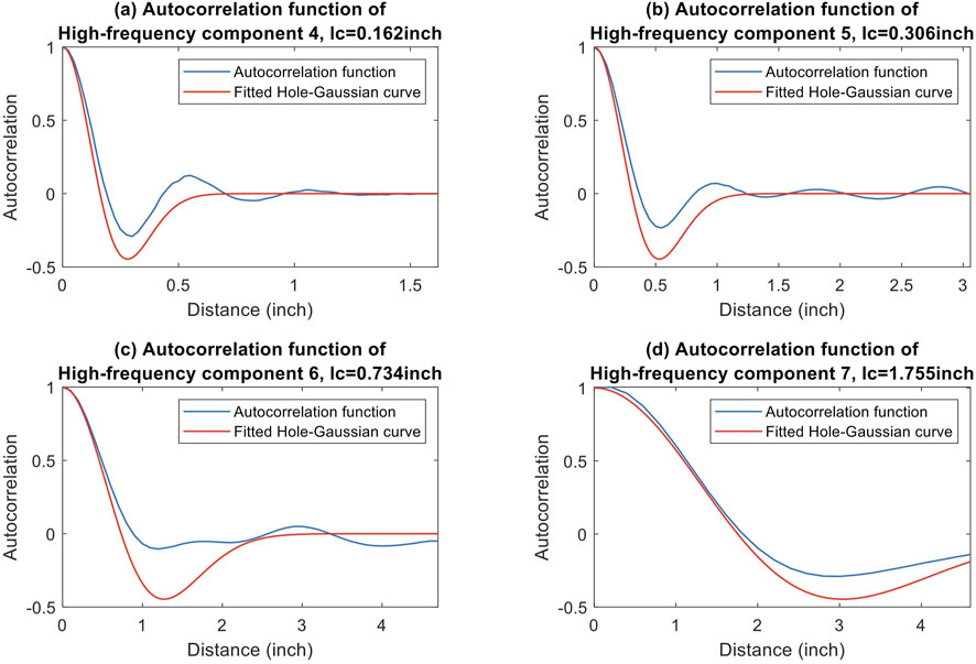
Figure 11. (a–d) Hole-Gaussian autocorrelation functions of high-frequency components 4 to 7, respectively, of corroded surface 1.

The fitted Hole-Gaussian autocorrelation model for high-frequency components 4 to 7 of corroded surface 1 are plotted in red in Figure 11, and the fitted correlation lengths, l_c, for the high-frequency components of all five corroded surfaces are listed in Table 2. The correlation length of the high-frequency components approximately doubles for each increase in high-frequency component level due to the Lanczos3 filter used to extract each component. Similar to the standard deviation of the height values in the high-frequency components, l_c is fitted as a reciprocal function of the cutoff frequency of the Lanczos3 filter, y = c/x, where the fitted value for c is 0.283, as plotted in Figure 10b. The variation in l_c is much smaller than the variation in the standard deviation of height values in the high-frequency components, especially for components 4 and 5. This is because the correlation length is not significantly affected by corrosion intensity. For a defined cutoff frequency of the Lanczos3 filter, the corresponding l_c value does not change much. The increased variation in l_c for components 6 and 7 is mainly because insufficient waves are captured due to the surface size.

Table 2

Table 2. The correlation length of high-frequency components 4 to 7 for all the corroded surfaces.

3.3 Characterizing the low-frequency component

Bivariate Lagrange polynomials are constructed to characterize the low-frequency components based on n-section points sampling and Gauss points sampling. Three different-sized grid-pattern point sample sets, 3 × 3, 4 × 4, and 5 × 5, are created for each sampling method. Lagrange polynomials are then constructed based on Equations 5, 6. The accuracy of the constructed polynomials is evaluated based on relative volume error (RVE) and normalized root mean square error (NRMSE) (Shcherbakov et al., 2013), as shown in Table 3. The RVE (Equation 9) is the ratio of the difference between the volumes of the constructed surface and the low-frequency component to the volume of the low-frequency component. It measures the first-moment accuracy of the fitted polynomial. The NRMSE (Equation 10) is the ratio of the root mean square error to the mean value of the original low-frequency component, evaluating the second-moment accuracy of the fitted polynomial.

$\text{RVE}=\frac{{\displaystyle {\sum }_{i=1}^n}\left(f\left(x_i,y_i\right)-z_i\right)}{{\displaystyle {\sum }_{i=1}^n}{z}_i}\times 100\%(9)$

$\text{NRMSE}=\frac{\sqrt{\frac{1}{n}{\sum }_{i=1}^n{\left(f\left(x_i,y_i\right)-z_i\right)}^2}}{\frac{1}{n}\left|{\displaystyle {\sum }_{i=1}^n}{z}_i\right|}\times 100\%(10)$

Table 3

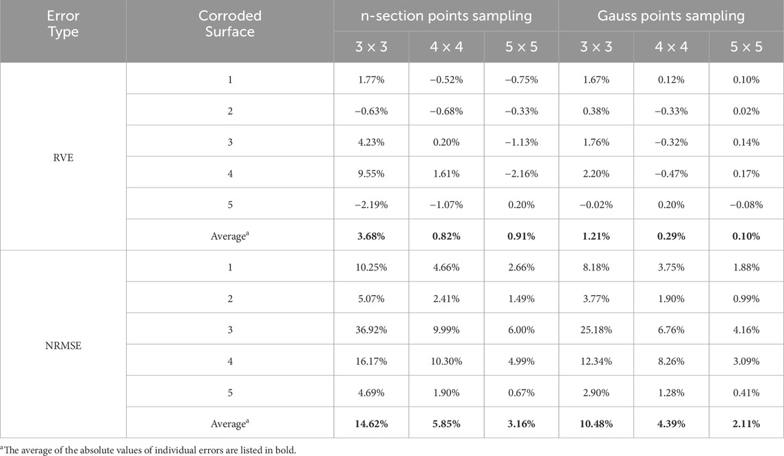
Table 3. Errors between the low-frequency components and the Lagrange polynomials constructed using n-section points sampling and Gauss points sampling.

The average of the absolute values of the RVE for the n-section points sampling with 3 × 3, 4 × 4, and 5 × 5 sample points are 3.68%, 0.82%, and 0.91%, respectively, and for the Gauss points sampling are 1.21%, 0.29%, and 0.10%, respectively. The averages of the NRMSE for the n-section points sampling are 14.62%, 5.85%, and 3.16%, and for the Gauss points sampling are 10.48%, 4.39%, and 2.11%. As expected, both average errors decreased with the increase of polynomial degrees. When the same sample point size is used, the error for Gauss points sampling is smaller than for n-section points sampling. Thus, a 4 × 4 Gauss points set is selected to model the low-frequency components in this case study. For a 4 × 4-point set, the polynomial has a degree of 3 for both x and y. Therefore, the polynomial can be represented using a 4 × 4 coefficients matrix A, in which a_ij is the coefficient of the polynomial term x^jyⁱ.

$\mathit{A}=\left[\begin{array}{cc}\begin{array}{cc}{a}_{00}& a_{01}\\ a_{10}& a_{11}\end{array}& \begin{array}{cc}{a}_{02}& a_{03}\\ a_{12}& a_{13}\end{array}\\ \begin{array}{cc}{a}_{20}& a_{21}\\ a_{30}& a_{31}\end{array}& \begin{array}{cc}{a}_{22}& a_{23}\\ a_{32}& a_{33}\end{array}\end{array}\right]$

Figure 12 shows the low-frequency components and the bivariate Lagrange polynomials constructed using a 4 × 4 Gauss sample point set for the five corroded surfaces. When the low-frequency component is concave in the entire corroded region (corroded surfaces 1, 2, and 5), the fitted Lagrange polynomial can accurately represent the low-frequency component with NRMSE values between 1% and 4%. However, the NRMSE is relatively large (6%–9%) when the low-frequency component has a concave shape in a local region, as is the case for corroded surfaces 3 and 4.

Figure 12

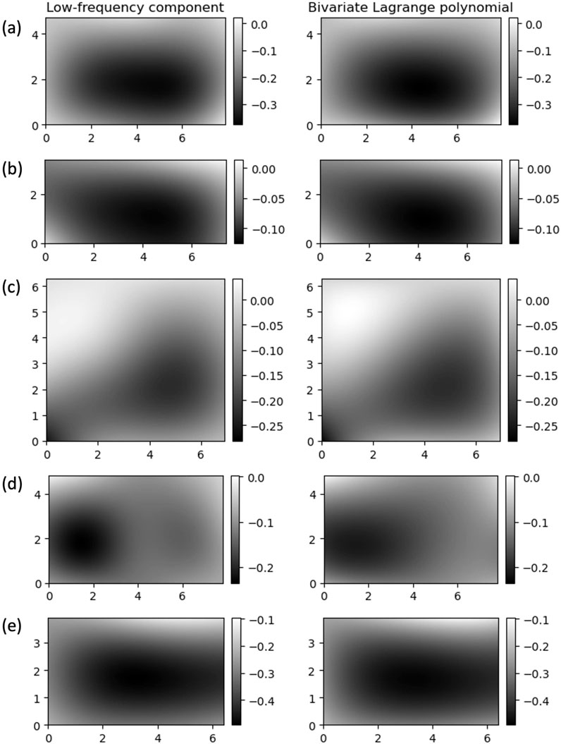
Figure 12. The low-frequency components (left) and the fitted bivariate Lagrange polynomials using a 4 × 4 Gauss point set (right) for the five corroded surfaces (inch) – (a–e) corroded surfaces 1–5.

4 Conclusion

This paper proposed a novel method for characterizing the geometry of locally corroded steel surfaces. The approach decomposes a corroded surface into multilevel high-frequency components and a single low-frequency component using Lanczos3 filters, and then characterizes these components using statistical models and polynomial functions. The methodology was successfully evaluated on five real corroded surfaces obtained from the 3D scanning of corroded bridge girder ends from a 57-year-old in-service bridge.

The analysis of the high-frequency components revealed that the height values follow a normal distribution and that the ACFs are well represented by a Hole-Gaussian model. In addition, two reciprocal functions were observed to describe the relationship between the statistical features and the cutoff frequencies of the Lanczos3 filters. Specifically, the standard deviation of the height values is proportional to a constant, b, divided by the cutoff frequency of the Lanczos filter, and the correlation length is proportional to a constant, c, divided by the same cutoff frequency. For the low-frequency component, a bivariate Lagrange polynomial constructed from a 4 × 4 Gauss point sampling set effectively captured the underlying surface geometry with low normalized root mean square errors.

This decomposition provides a comprehensive characterization of corrosion damage by capturing both fine textures and the overall shape and eccentricity of the corroded surface. Because the original surface can be reconstructed from its frequency components, the method also enables the generation of artificial corroded surfaces, addressing challenges in large-scale data collection for computational corrosion damage investigations. Specifically, the artificially generated corroded surfaces may be used to train neural networks that predict the residual bearing capacity for the intricate surface geometry of real corroded surfaces (Zhang et al., 2023). The proposed method also helps overcome computational challenges associated with large-matrix representations of corrosion by reducing the surface description to a small, information-rich set of parameters.

While the results are promising, the methodology was only applied to five 3D scans of locally corroded surfaces. Therefore, the resulting statistical analyses should be considered carefully. Future research should validate the approach on a broader range of surfaces that span various exposure durations and corrosion patterns. In addition, the first three high-frequency components—affected primarily by noise due to the scanner accuracy and the filter cutoff frequencies—were excluded from the analysis, which limits the method’s ability to characterize fine surface textures. We further note that the use of k = 3 in the definition of the Lanczos filters was selected to balance the filter’s roll off with computational complexity. A more detailed sensitivity analysis of this parameter or the use of alternative surface filtering techniques (e.g., wavelet transforms) could clarify how variations in the filter design affect the decomposition results. Finally, while the criterion used to determine the number of high-frequency components extracted—where the filter’s wavelength is comparable to the surface size—produced good results in this study, future work should explore whether it remains optimal for larger and smaller scans.

Data availability statement

The raw data supporting the conclusions of this article will be made available by the authors, without undue reservation.

Author contributions

TZ: Conceptualization, Data curation, Formal Analysis, Investigation, Methodology, Software, Validation, Visualization, Writing – original draft, Writing – review and editing. MV: Visualization, Writing – review and editing. AZ: Conceptualization, Funding acquisition, Methodology, Project administration, Resources, Supervision, Writing – review and editing. AB: Conceptualization, Methodology, Writing – review and editing.

Funding

The author(s) declare that financial support was received for the research and/or publication of this article. This work was supported by funding (SPR-2310) from the Connecticut Department of Transportation.

Conflict of interest

The authors declare that the research was conducted in the absence of any commercial or financial relationships that could be construed as a potential conflict of interest.

Generative AI statement

The authors declare that Gen AI was used in the creation of this manuscript. In preparation of this article, the authors used OpenAI’s GPT models as a writing assistant to check grammar and enhance the clarity of the written text. These models were used with extreme oversight and care. The authors take full responsibility for the content presented herein.

Publisher’s note

All claims expressed in this article are solely those of the authors and do not necessarily represent those of their affiliated organizations, or those of the publisher, the editors and the reviewers. Any product that may be evaluated in this article, or claim that may be made by its manufacturer, is not guaranteed or endorsed by the publisher.

References

Ababou, R., Bagtzoglou, A. C., and Wood, E. F. (1994). On the condition number of covariance matrices in kriging, estimation, and simulation of random fields. Math. Geol. 26, 99–133. doi:10.1007/BF02065878

CrossRef Full Text | Google Scholar

Alemdar, F., Nagati, D., Matamoros, A., Bennett, C., and Rolfe, S. (2014). Repairing distortion-induced fatigue cracks in steel bridge girders using angles-with-plate retrofit technique. I: physical simulations. J. Struct. Eng. 140. doi:10.1061/(ASCE)ST.1943-541X.0000876

CrossRef Full Text | Google Scholar

Appuhamy, J. M. R. S., Kaita, T., Ohga, M., and Fujii, K. (2011). Prediction of residual strength of corroded tensile steel plates. Int. J. Steel Struct. 11, 65–79. doi:10.1007/S13296-011-1006-6

CrossRef Full Text | Google Scholar

Artec3D (2019). Professional 3D scanning solutions.

Google Scholar

ASCE (2025). 2025 Infrastructure report card.

Google Scholar

Bagtzoglou, A. C., and Hossain, F. (2009). Radial basis function neural network for hydrologic inversion: an appraisal with classical and spatio-temporal geostatistical techniques in the context of site characterization. Stoch. Environ. Res. Risk Assess. 23, 933–945. doi:10.1007/s00477-008-0262-2

CrossRef Full Text | Google Scholar

Bao, A., Guillaume, C., Satter, C., Moraes, A., Williams, P., Kelly, T., et al. (2021). Testing and evaluation of web bearing capacity of corroded steel bridge girders. Eng. Struct. 238, 112276. doi:10.1016/j.engstruct.2021.112276

CrossRef Full Text | Google Scholar

Das, A., Ichi, E., and Dorafshan, S. (2023). Image-based corrosion detection in ancillary structures. Infrastructures (Basel) 8, 66. doi:10.3390/infrastructures8040066

CrossRef Full Text | Google Scholar

Deliang, K., Biao, N., and Shanhua, X. (2021). Random field model of corroded steel plate surface in neutral salt spray environment. KSCE J. Civ. Eng. 25, 2651–2661. doi:10.1007/s12205-021-1249-5

CrossRef Full Text | Google Scholar

Duchon, C. E. (1979). Lanczos filtering in one and two dimensions. J. Appl. Meteorology 18, 1016–1022. doi:10.1175/1520-0450(1979)018<1016:lfioat>2.0.co;2

CrossRef Full Text | Google Scholar

Forkan, A. R. M., Kang, Y.-B., Jayaraman, P. P., Liao, K., Kaul, R., Morgan, G., et al. (2022). CorrDetector: a framework for structural corrosion detection from drone images using ensemble deep learning. Expert Syst. Appl. 193, 116461. doi:10.1016/j.eswa.2021.116461

CrossRef Full Text | Google Scholar

Guo, T., Zhang, T., Lim, E., Lopez-Benitez, M., Ma, F., and Yu, L. (2022). A review of wavelet analysis and its applications: challenges and opportunities. IEEE Access 10, 58869–58903. doi:10.1109/ACCESS.2022.3179517

CrossRef Full Text | Google Scholar

Hain, A., Zaghi, A. E., Kamali, A., Zaffetti, R. P., Overturf, B., and Pereira, F. E. (2019). Applicability of 3-D scanning technology for section loss assessment in corroded steel beams. Transp. Res. Rec. J. Transp. Res. Board 2673, 271–280. doi:10.1177/0361198119832887

CrossRef Full Text | Google Scholar

Hain, A., Zhang, T., and Zaghi, A. E. (2021). “Estimation of the residual bearing capacity of corrosion damaged bridge beams using 3D scanning and finite element analysis,” in Bridge maintenance, safety, management, life-cycle sustainability and innovations. Editors H. Yokota, and D. M. Frangopol (London: CRC Press).

CrossRef Full Text | Google Scholar

Htun, M. M., Kawamura, Y., and Ajiki, M. (2013). “A study on random field model for representation of corroded surface,” in Analysis and design of marine structures - proceedings of the 4th international conference on marine structures, MARSTRUCT 2013, 545–553.

Google Scholar

Kanakamedala, D., Seo, J., Varma, A. H., Connor, R. J., and Tarasova, A. (2023). Shear and bearing capacity of corroded steel beam bridges and the effects on load rating. West Lafayette, Indiana. doi:10.5703/1288284317634

CrossRef Full Text | Google Scholar

Kayser, J. R., and Nowak, A. S. (1989). Reliability of corroded steel girder bridges. Struct. Saf. 6, 53–63. doi:10.1016/0167-4730(89)90007-6

CrossRef Full Text | Google Scholar

Kere, K. J., and Huang, Q. (2019). Life-cycle cost comparison of corrosion management strategies for steel bridges. J. Bridge Eng. 24. doi:10.1061/(ASCE)BE.1943-5592.0001361

CrossRef Full Text | Google Scholar

Khurram, N., Sasaki, E., Katsuchi, H., and Yamada, H. (2014a). Experimental and numerical evaluation of bearing capacity of steel plate girder affected by end panel corrosion. Int. J. Steel Struct. 14, 659–676. doi:10.1007/s13296-014-3023-8

CrossRef Full Text | Google Scholar

Khurram, N., Sasaki, E., Kihira, H., Katsuchi, H., and Yamada, H. (2014b). Analytical demonstrations to assess residual bearing capacities of steel plate girder ends with stiffeners damaged by corrosion. Struct. Infrastructure Eng. 10, 69–79. doi:10.1080/15732479.2012.697904

CrossRef Full Text | Google Scholar

Kleijnen, J. P. C. (2009). Kriging metamodeling in simulation: a review. Eur. J. Oper. Res. 192, 707–716. doi:10.1016/j.ejor.2007.10.013

CrossRef Full Text | Google Scholar

Lanczos, C. (1988). Applied analysis. Cour. Corp.

Google Scholar

Leach, R. (2013). Characterisation of areal surface texture. Heidelberg: Berlin: Springer.

Google Scholar

Lin, H.-C., Wang, L.-L., and Yang, S.-N. (1997). Extracting periodicity of a regular texture based on autocorrelation functions. Pattern Recognit. Lett. 18, 433–443. doi:10.1016/S0167-8655(97)00030-5

CrossRef Full Text | Google Scholar

Liu, C., Miyashita, T., and Nagai, M. (2011). Analytical study on shear capacity of steel I-girders with local corrosion nearby supports. Procedia Eng. 14, 2276–2284. doi:10.1016/j.proeng.2011.07.287

CrossRef Full Text | Google Scholar

McMullen, K. F., and Zaghi, A. E. (2020). Experimental evaluation of full-scale corroded steel plate girders repaired with UHPC. J. Bridge Eng. 25. doi:10.1061/(ASCE)BE.1943-5592.0001535

CrossRef Full Text | Google Scholar

Melchers, R. E., Ahammed, M., Jeffrey, R., and Simundic, G. (2010). Statistical characterization of surfaces of corroded steel plates. Mar. Struct. 23, 274–287. doi:10.1016/j.marstruc.2010.07.002

CrossRef Full Text | Google Scholar

Mokhtari, M., and Melchers, R. E. (2018). A new approach to assess the remaining strength of corroded steel pipes. Eng. Fail Anal. 93, 144–156. doi:10.1016/j.engfailanal.2018.07.011

CrossRef Full Text | Google Scholar

Munawar, H., Ullah, F., Shahzad, D., Heravi, A., Qayyum, S., and Akram, J. (2022). Civil infrastructure damage and corrosion detection: an application of machine learning. Buildings 12, 156. doi:10.3390/buildings12020156

CrossRef Full Text | Google Scholar

Nurunnabi, A., Belton, D., and West, G. (2014). Robust statistical approaches for local planar surface fitting in 3D laser scanning data. ISPRS J. Photogrammetry Remote Sens. 96, 106–122. doi:10.1016/j.isprsjprs.2014.07.004

CrossRef Full Text | Google Scholar

Pérez-Brokate, C. F., di Caprio, D., Féron, D., de Lamare, J., and Chaussé, A. (2016). Three dimensional discrete stochastic model of occluded corrosion cell. Corros. Sci. 111, 230–241. doi:10.1016/j.corsci.2016.04.009

CrossRef Full Text | Google Scholar

Prucz, Z., and Kulicki, J. M. (1998). Accounting for effects of corrosion section loss in steel bridges. Transp. Res. Rec. J. Transp. Res. Board 1624, 101–109. doi:10.3141/1624-12

CrossRef Full Text | Google Scholar

Qin, G., Xu, S., Yao, D., and Zhang, Z. (2016). Study on the degradation of mechanical properties of corroded steel plates based on surface topography. J. Constr. Steel Res. 125, 205–217. doi:10.1016/j.jcsr.2016.06.018

CrossRef Full Text | Google Scholar

Salunkhe, A. A., Gobinath, R., Vinay, S., and Joseph, L. (2022). Progress and trends in image processing applications in civil engineering: opportunities and challenges. Adv. Civ. Eng. 2022. doi:10.1155/2022/6400254

CrossRef Full Text | Google Scholar

Sharifi, Y., and Tohidi, S. (2014). Ultimate capacity assessment of web plate beams with pitting corrosion subjected to patch loading by artificial neural networks. Adv. Steel Constr. 10, 325–350. doi:10.18057/ijasc.2014.10.3.5

CrossRef Full Text | Google Scholar

Shcherbakov, M. V., Brebels, A., Shcherbakova, N. L., Tyukov, A. P., Janovsky, T. A., and Kamaev, V. A. (2013). A survey of forecast error measures. World Appl. Sci. J. 24, 171–176.

Google Scholar

Shojai, S., Schaumann, P., Braun, M., and Ehlers, S. (2022). Influence of pitting corrosion on the fatigue strength of offshore steel structures based on 3D surface scans. Int. J. Fatigue 164, 107128. doi:10.1016/j.ijfatigue.2022.107128

CrossRef Full Text | Google Scholar

Stępień, J., di Caprio, D., and Stafiej, J. (2019). 3D simulations of the metal passivation process in potentiostatic conditions using discrete lattice gas automaton. Electrochim Acta 295, 173–180. doi:10.1016/j.electacta.2018.09.113

CrossRef Full Text | Google Scholar

Strang, G., and Nguyen, T. (1996). Wavelets and filter banks. Wellesley, MA: Wellesley-Cambridge Press.

Google Scholar

Sun, M., Zhang, Y., Cui, X., Fan, F., Zeng, B., and Dai, K. (2025). Experimental and numerical simulation study of tensile mechanical properties of corroded carbon steel utilizing galvanostatic corrosion and 3D scanning. Structures 71, 108132. doi:10.1016/j.istruc.2024.108132

CrossRef Full Text | Google Scholar

Swarztrauber, P. N. (2003). On computing the points and weights for Gauss--legendre quadrature. SIAM J. Sci. Comput. 24, 945–954. doi:10.1137/S1064827500379690

CrossRef Full Text | Google Scholar

Teixeira, Â. P., and Soares, C. G. (2008). Ultimate strength of plates with random fields of corrosion. Struct. Infrastructure Eng. 4, 363–370. doi:10.1080/15732470701270066

CrossRef Full Text | Google Scholar

Tohidi, S., and Sharifi, Y. (2016). Load-carrying capacity of locally corroded steel plate girder ends using artificial neural network. Thin-Walled Struct. 100, 48–61. doi:10.1016/j.tws.2015.12.007

CrossRef Full Text | Google Scholar

Tzortzinis, G., Ai, C., Breña, S. F., and Gerasimidis, S. (2022). Using 3D laser scanning for estimating the capacity of corroded steel bridge girders: experiments, computations and analytical solutions. Eng. Struct. 265, 114407. doi:10.1016/j.engstruct.2022.114407

CrossRef Full Text | Google Scholar

Tzortzinis, G., Knickle, B. T., Bardow, A., Breña, S. F., and Gerasimidis, S. (2021a). Strength evaluation of deteriorated girder ends. I: experimental study on naturally corroded I-beams. Thin-Walled Struct. 159, 107220. doi:10.1016/j.tws.2020.107220

CrossRef Full Text | Google Scholar

Tzortzinis, G., Knickle, B. T., Bardow, A., Breña, S. F., and Gerasimidis, S. (2021b). Strength evaluation of deteriorated girder ends. II: numerical study on corroded I-beams. Thin-Walled Struct. 159, 107216. doi:10.1016/j.tws.2020.107216

CrossRef Full Text | Google Scholar

van Beers, W. C. M., and Kleijnen, J. P. C. (2003). Kriging for interpolation in random simulation. J. Operational Res. Soc. 54, 255–262. doi:10.1057/palgrave.jors.2601492

CrossRef Full Text | Google Scholar

Weiss, V., Andor, L., Renner, G., and Várady, T. (2002). Advanced surface fitting techniques. Comput. Aided Geom. Des. 19, 19–42. doi:10.1016/S0167-8396(01)00086-3

CrossRef Full Text | Google Scholar

Werner, W. (1984). Polynomial interpolation: Lagrange versus Newton. Math. Comput. 43, 205. doi:10.2307/2007406

CrossRef Full Text | Google Scholar

Woodward, P. M., and Davies, I. L. (1952). “Information theory and inverse probability in telecommunication,” in Proceedings of the IEE - Part III: radio and communication engineering, 37–44. doi:10.1049/pi-3.1952.0011

CrossRef Full Text | Google Scholar

Yan, K., Liu, G., Li, Q., Jiang, C., Ren, T., Li, Z., et al. (2024). Corrosion characteristics and evaluation of galvanized high-strength steel wire for bridge cables based on 3D laser scanning and image recognition. Constr. Build. Mater 422, 135845. doi:10.1016/j.conbuildmat.2024.135845

CrossRef Full Text | Google Scholar

Zhang, T., Vaccaro, M., and Zaghi, A. E. (2023). Application of neural networks to the prediction of the compressive capacity of corroded steel plates. Front. Built Environ. 9. doi:10.3389/fbuil.2023.1156760

CrossRef Full Text | Google Scholar

Zhang, T., and Zaghi, A. E. (2023). Estimation of the residual bearing strength of corroded bridge girders using 3D scan data. Thin-Walled Struct. 188, 110798. doi:10.1016/j.tws.2023.110798

CrossRef Full Text | Google Scholar

Zhu, J. S., Guo, X. Y., and Kang, J. F. (2018). “3D cellular automata based numerical simulation of atmospheric corrosion process on weathering steel,” in Maintenance, safety, risk, management, and life-cycle performance of bridges. Editors N. Powers, D. M. Frangopol, R. Al-Mahaidi, and C. Caprani (Leiden, The Netherlands: CRC Press), 1791–1797.

CrossRef Full Text | Google Scholar

Zimmerman, D., Pavlik, C., Ruggles, A., and Armstrong, M. P. (1999). An experimental comparison of ordinary and universal kriging and inverse distance weighting. Math. Geol. 31, 375–390. doi:10.1023/A:1007586507433

CrossRef Full Text | Google Scholar

Zmetra, K. M., McMullen, K. F., Zaghi, A. E., and Wille, K. (2017). Experimental study of UHPC repair for corrosion-damaged steel girder ends. J. Bridge Eng. 22. doi:10.1061/(ASCE)BE.1943-5592.0001067

CrossRef Full Text | Google Scholar

Nomenclature

Abbreviations

ACF Autocorrelation function

CV Coefficient of variation

NRMSE Normalized root mean square error

RVE Relative volume error

Parameters and Constants

A: Coefficient matrix of the bivariate Lagrange polynomial

b Constant in the reciprocal fit for standard deviation

c Constant in the reciprocal fit for correlation length

d Distance between two points in a random field

k Lanczos window parameter

L Pixel size

l_c Correlation length

l Lanczos filter level

M Length/width of the original corroded surface

m Degree of the bivariate Lagrange polynomial in the x direction

μ Mean of height values in a random field

N Side length of the filter

n Degree of the bivariate Lagrange polynomial in the y direction

σ Standard deviation of height values in a random field

v_l Discretized Lanczos filter of level l

Functions

f(x, y) Equation of the bivariate Lagrange polynomial

l_i,j(x, y) Lagrange basis

ρ(d) Autocorrelation between two points in a random field a distance d apart

S(d) Hole-Gaussian autocorrelation between two points a distance d apart