Fast and intelligent detection of concrete cracks based on sound signals and convolutional neural network

Introduction: The traditional crack detection method usually requires a tedious process of sensor installation and removal, which seriously affects the efficiency of concrete structure management and maintenance.

Methods: For this reason, this paper develops a fast concrete crack detection method based on percussion with an improved convolutional neural network (CNN). By utilizing the percussion method, the sensors do not need to be coupled and installed on the concrete structure, which saves a lot of processes. The sound signals generated by percussion are collected by acoustic pressure sensors, while multiple data enhancement techniques are applied to enrich the data volume and diversity of the collected signals. The Mel-frequency cepstral coefficient (MFCC) of the sound signals are then extracted as inputs to the improved CNN model. The CNN used is mainly applied to initialize the weights by applying the transfer learning technique, and the Squeeze-and-Excitation Networks (SENet) attention mechanism is embedded to improve the model’s focus on important features. Finally, comparative experiments with different frame lengths, different models and different signal-to-noise ratios (SNR) are conducted using the improved CNN.

Results: The results show that the model validation process has the least loss and highest accuracy when the input frame length is 1024. The improved CNN has good feature learning ability for MFCC of percussion sound signals for effective recognition of concrete cracks. Compared with Resnet18, random forest and long short-term memory networks, the improved CNN has superior recognition accuracy and stability, and shows better noise robustness in high signal-to-noise ratio (SNR: −6 db∼6 db) environments.

Discussion: Therefore, the proposed method has a high potential for future crack detection in concrete structures.

1 Introduction

It is well known that concrete, as an important construction material, is one of the most widely used materials in the field of civil engineering. However, due to various reasons such as environmental and loading effects, infrastructures composed mainly of concrete such as roads, bridges and dams are highly susceptible to cracking (Chen and Mahadevan, 2008). Cracking of concrete, on the one hand, affects the aesthetics and durability of the structure, and even reduces the structural bearing capacity and shortens the service life (Kaufmann and Marti, 1998). On the other hand, moisture and corrosion factors (chloride ions, etc.) will enter the concrete interior through the cracks and erode the internal reinforcing bars (Gowripalan et al., 2000), which accelerates the deterioration of the overall structural performance (Matallah and La Borderie, 2009) and brings about costly repair and maintenance as well as serious safety hazards. Therefore, crack detection in concrete structures plays a crucial role in damage assessment and post-care of the structure.

The main concrete crack detection methods include ultrasonic method (Pahlavan et al., 2018), ground-penetrating radar method (Rasol et al., 2020), infrared method (Tashan and Al-Mahaidi, 2014), impact echo method (Hsiao et al., 2008), acoustic emission method (Ohno and Ohtsu, 2010), and image machine vision method (Kim and Cho, 2018). Although these methods show great potential in the detection of concrete crack length, depth, width, etc., they all have certain limitations. Ultrasonic methods often difficult to accurately characterize cracks qualitatively and quantitatively. Ground-penetrating radar methods can be used to determine the shape of crack defects, but the accuracy of detection depends on the skill level of the inspector and is both time-consuming and expensive (Tosti and Ferrante, 2020). The infrared method is unable to detect microcracks within the structure (Sirca and Adeli, 2018). The accuracy of the impact echo method is susceptible to strength. The acoustic emission method is very sensitive to the material and susceptible to electromechanical noise interference (Goszczyńska et al., 2012). The image machine vision method has been developed in recent years as an intelligent detection technique, but the image of concrete cracks acquired by the camera contains a lot of noise that can cause serious interference with the accuracy of crack recognition, such as uneven lighting, surface stains and unevenness (Koch et al., 2015). Therefore, it is necessary to demand a simple, cheap and fast method to detect cracks in concrete.

The percussion method is easy to operate, does not require expensive testing equipment, and has been applied to the defect detection of structures for a long time. In the past, the structural vibration caused by percussion was mainly used to realize the accurate assessment of structural damage (Kubojima et al., 2018), and the sound signal caused by percussion was usually only used as an auxiliary evaluation index because the discriminative results based on the sound signal mainly relied on the experience of the inspectors (Cawley and Adams, 1988). However, with the rapid development of computer technology and artificial intelligence algorithms, percussion-induced sound signals have attracted the attention of more and more scholars. This is mainly because the development of signal processing technology makes it possible to extract more acoustic features from the collected sound signals (Kong et al., 2018) and use artificial intelligence algorithms to find the complex mapping relationship between acoustic features and structural damage more easily (Wang et al., 2021a), thus greatly improving the accuracy of structural detection and evaluation. Therefore, in recent years, methods using the combination of percussion sound signals and artificial intelligence have been developed in many fields. Zheng et al. (2019) used a microphone to capture the sound signals of the percussion process and extracted the Mel-frequency cepstral coefficient (MFCC) as inputs to a Support Vector Machine (SVM) model to categorize the water content of concrete. The results showed that the proposed method obtained more than 98% accuracy. Wang et al. (2021b) developed a bolt-loosening detection method using MFCC and memory-enhanced neural network, and initially explored the potential of the method for automation in the real industry by using a robotic arm to replace the manual operation for percussion. Further, they also proposed a new method of convolutional bi-directional long and short-term memory model combined with MFCC, and verified the effectiveness of the method in scaffolding loosening detection through indoor experiments (Wang and Song, 2020). Chen et al. (2022) conducted a series of percussion tests on wooden posts with different cavity volumes and environmental variations to classify wood cavities using sound features and deep neural networks. The results show that the proposed method has good classification performance and generalization regardless of the knocking location, wood post-cross-section and environment changes. Recently, Chen et al. proposed three different recognition methods based on the percussion method, namely, power spectral density (PSD) and SVM (Chen et al., 2020a), PSD and decision making (DT) (Chen et al., 2020b), and wavelet transform (WT and improved convolutional neural network (Chen et al., 2023), respectively, to validate the potential of the proposed method in improving the accuracy and efficiency of the detection by carrying out percussion experiments on steel pipe concretes with different degrees of voids.

This paper explores an innovative method based on percussion for identifying crack widths in concrete structures. The method starts by percussing the concrete surface using a hammer, and the acoustic signals generated by the percussion process are captured using an acoustic pressure transducer. Then data enhancement technique is used to increase the data volume and diversity of the signals. Next, MFCC is extracted as an input feature and an improved convolutional neural network (CNN) model is built by introducing transfer learning and Squeeze-and-Excitation Networks (SENet) attention mechanism to recognize the crack width. In order to verify the effectiveness of the proposed method, two concrete specimens encased in steel tubes were prepared in this paper to achieve different cracking widths by applying different load displacements. Under different cracking widths, hammers were used to percuss 150 times respectively, and the sound signals of the percussion process were recorded. Multiple data enhancement techniques were utilized to enrich the data volume and diversity of the signals. Then, the data with different cracking widths are divided into training, validation and testing sets according to the ratio of 4:1:5, respectively. The results show that the proposed method obtains more than 98% recognition accuracy and exhibits good noise robustness in indoor experiments. The rest of the paper is organized as follows: Section 2 describes the basic theories used in this paper, including MFCC, CNN, transfer learning and SENet. Section 3 describes the specific structure and workflow of the proposed model. Section 4 presents the validation of the proposed method. Section 5 is the conclusion.

2 Theoretical foundation

2.1 Mel-frequency cepstral coefficient (MFCC)

The MFCC characterization describes the ability of the human auditory system to perceive sound as a linear function of frequency below 1 kHz and logarithmically above 1 kHz. According to the auditory excitation of the human ear, the original frequencies are nonlinearly mapped by a Mel filter bank, so as to transform the original frequencies to the Mel domain that can be perceived by human hearing (Murty and Yegnanarayana, 2005). The relationship between the Mel frequency and the frequency of the sound signal can be described by using Equation 1, where $\lambda$ stands for the frequency.

$\text{Mel}\left(f\right)=2595\lg \left(1+\frac{\lambda }{700}\right)(1)$

The computational flow of MFCC includes pre-emphasis, windowing and framing, and discrete Fourier transform (DFT) as follows:

(1) Pre-emphasis. For sound signals $x\left(n\right)$, $1\le \mathrm{n}\le N$, the following formula (Equation 2) can be used for pre-emphasis:

$X\left(\mathrm{n}\right)=\mathrm{x}\left(\mathrm{n}\right)-\gamma \mathrm{x}\left(\mathrm{n}-1\right)(2)$

Where, $X\left(\mathrm{n}\right)$ is the pre-emphasized output signal; $\gamma$ is the pre-emphasis coefficient of the sound signals.

(2) Framing and windowing. Framing of the sound signal is to add a window function of finite length to the acquired sound signal. The commonly used window functions are usually rectangular window, Hanning window, and Hamming window, which are used in this paper with Equations 3, 4:

$S\left(n\right)=\phi \left(n\right)X\left(n\right)(3)$

$\phi \left(n\right)=0.54-0.46\cos \left(2\pi \frac{n-1}{N-1}\right)(4)$

Where, $S\left(n\right)$ is the smoothed signal with Hamming window; $\phi \left(n\right)$ is the Hamming window.

(3) Discrete Fourier Transform (DFT). In order to obtain the linear spectrum of the sound signal, it is necessary to perform the DFT on the signal after windowing to obtain the corresponding spectrum, as follows with Equation 5:

$Q\left(k\right)={\displaystyle \sum _0^{N-1}}S\left(n\right)e^{-\frac{j2\pi nk}{N}}\left(0\le k\le N-1\right)(5)$

(4) Mel frequency filtering. Further, the spectrum from step (3) is passed through the Mel filter bank to obtain a Mel spectrum, as follows Equation 6:

$H_m\left(k\right)=\left\{\begin{array}{ll}0& k<y\left(m-1\right)\\ \frac{k-y\left(m-1\right)}{y\left(m\right)-y\left(m-1\right)}& y\left(m-1\right)\le k\le y\left(m\right)\\ \frac{y\left(m+1\right)-k}{y\left(m+1\right)-y\left(m\right)}& y\left(m\right)<k\le y\left(m+1\right)\\ 0& k>y\left(m+1\right)\end{array}\right.(6)$

Where, 0 ≤ m ≤ M, M is the total number of filters; $y\left(·\right)$ is the center frequency of the mth filter.

(5) Logarithmic transformation. Next, the logarithmic energy of the signal is calculated using Equation 7:

$S\left(m\right)=\ln \left({\displaystyle \sum _0^{N-1}}|{\left|Q\left(k\right)\right|}^2|H_m|\left(k\right)\right)(7)$

(6) Discrete Cosine Transform (DCT). Finally, the DCT is performed on the logarithmic energy to obtain the MFCC by Equation 8:

$C\left(n\right)={\displaystyle \sum _1^{M-1}}S\left(m\right)\cos \left(\frac{\pi n\left(m+1/2\right)}{M}\right)(8)$

The specific implementation process is shown in Figure 1.

Figure 1

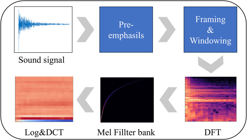
Figure 1. MFCC flow chart.

2.2 Convolutional neural network (CNN)

CNN is a typical deep-learning network with different functional layers including convolutional, pooling, and fully connected layers (Yang and Huo, 2022). CNN networks make it possible to greatly reduce the number of their parameters without losing feature expressiveness by sharing weights.

2.2.1 Convolutional layer

A convolutional layer is the core module of CNN, which performs convolution operation on input feature maps by convolution kernel and computes output feature maps using the activation function. The convolution operation can be represented by Equation 9:

$y_{i,j}=f\left(b_j+{\displaystyle \sum _i}{k}_j*x_i\right)(9)$

Where $y_{i,j}$ is the output of the convolutional layer, $f\left(·\right)$ is the activation function, $b_j$ is the bias, $k_j$ is the convolutional kernel, $*$ is the sign of the convolutional operation, and $x_i$ is the input feature map, i and j represent the input channel index and output channel index respectively.

2.2.2 Pooling layer

The pooling layer scales and maps the input feature map through the pooling kernel to extract features while reducing the data dimensionality. Assuming the size of the pooling kernel is p*t and the input features are $x_i$, the output $y_i$ can be computed usually in Equation 10:

$y_i=f_{p*t}\left(x_i\right)(10)$

2.2.3 Full connectivity layer

The fully connected layer fully connects all neurons in the last pooling layer with the expression by Equation 1:

$O\left(x\right)=f\left(\mathbf{wx}+\mathbf{b}\right)(11)$

Where x is the input to the fully connected layer, w is the weight matrix, and b is the bias vector.

2.3 Transfer learning

Conventional methods usually require a large number of labeled data samples in the process of constructing a deep learning model and a long and complex tuning process before a model with relatively good performance can be obtained. In this paper, the percussion sound samples of concrete specimens with different cracking widths are limited, and the generalization ability of the resulting model is not high if it is trained directly on the existing samples. For this reason, we choose to complete the pre-training of the CNN model on the large dataset ImageNet. On this basis, a number of layers close to the input in the pre-trained model are frozen on the MFCC dataset of the enhanced percussion sound waves in this paper, and the weights of the network layers close to the output are fine-tuned to realize the migration learning and construct the backbone network.

2.4 SENet attention mechanism

In the process of machine learning, CNN also extracts the useless information in the feature map of the percussion spectrum and distributes it in certain channels of the feature map, which attracts the “attention” of the CNN network (Yao et al., 2022) and affects the recognition accuracy of the model. Therefore, we introduce the SENet attention mechanism, which can adaptively learn the importance of each feature channel and assign different weights to each channel of the feature map to adjust the importance of the feature channels, so that improves the accuracy of the model in recognizing the crack width (Yang et al., 2023), and the structure of the SENet is shown in Figure 2.

Figure 2

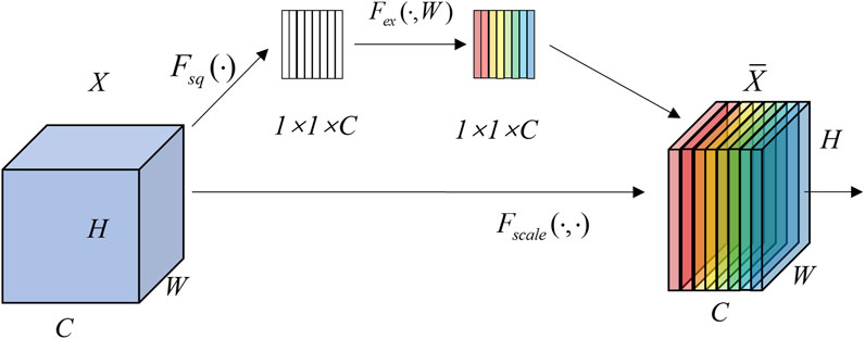
Figure 2. SENet structural model.

In the figure, C is the number of channels, H and W are the constant and width of the feature map, and X is the input feature map. SENet obtains the weights of each channel of the input feature map through two steps. In the first step, each feature channel is squeezed in the spatial dimension H × W by a global average pooling function with Equation 12:

$\mathbf{Z}={\mathbf{F}}_{\text{sq}}\left({\mathbf{X}}_{\mathrm{c}}\right)=\frac{1}{H\times W}{\displaystyle \sum _{i=1}^H}{\displaystyle \sum _{j=1}^W}{\mathbf{X}}_{\mathrm{c}}\left(i,j\right)(12)$

Where, $\mathrm{Z}$ is the weight generated by the compression operation.

In the second step, an excitation operation is performed to obtain the correlation between the feature channels. For this purpose, SENet applies a perceptron with an implicit layer containing C/L neurons. L is the scaling ratio. By choosing a suitable value of L, the network parameters can be reduced and the generalization ability of the network can be enhanced. In this paper, we draw on the results of the literature (Wang et al., 2019), and set the value of L to 16. Finally, the Sigmoid function is used to compute the feature channel weights. The calculation formula of the excitation operation can be expressed as Equation 13:

$S_{\mathrm{c}}=F_{\text{ex}}\left(Z,W\right)=\sigma \left(g\left(Z,W\right)\right)=\sigma \left(W_2\delta \left(W_{1}Z\right)\right)(13)$

Where $S_{\mathrm{c}}$ denotes the generated channel attention weights; $\sigma$ denotes the Sigmoid function; and $\delta$ denotes the ReLU function.

The expressions for the Sigmoid and ReLU functions are shown in Equations 14, 15, respectively:

$\sigma \left(\mathrm{x}\right)=\frac{1}{1+{\mathrm{e}}^{-x}}(14)$

$\delta \left(\mathrm{x}\right)=\left\{\begin{array}{l}\mathrm{x},\text{if}\mathrm{x}>0\\ 0,\text{otherwise}\end{array}\right.(15)$

Where e is a natural constant; x is the input value.

Finally, the generated channel attention weights are added to the original feature channels to realize the channel importance adjustment with Equation 16:

${\overline{\mathbf{X}}}_C={\mathbf{F}}_{\text{scale}}\left({\mathbf{X}}_{\mathrm{c}},{\mathbf{S}}_{\mathrm{c}}\right)={\mathbf{X}}_{\mathrm{c}}\otimes {\mathbf{S}}_{\mathrm{c}}(16)$

Where $\otimes$ denotes element-by-element multiplication; ${\overline{\mathbf{X}}}_C$ denotes the feature map after SENet processing.

3 Proposed crack identification model

In this paper, based on the traditional CNN model, transfer learning is used to pre-train the model to improve the training starting point. Then, the SENet attention mechanism is introduced to enhance the model’s focus on important features, proposing a novel concrete crack width recognition model, the Transfer Learning/SENet Optimised Convolutional Neural Network (TSCNN). Its network architecture is shown in Figure 3.

Figure 3

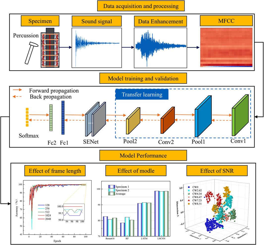
Figure 3. TSCNN crack width identification model.

As shown in Figure 3, the TSCNN model is mainly composed of 2 convolutional layers, 2 pooling layers, 1 SENet module, 2 fully connected layers and 1 Softmax classifier. The specific workflow of this model is as follows: firstly, the percussion sound signals under different crack widths are collected, and the percussion sound signals are processed with data enhancement; Then the local correlation features in the MFCC feature map are extracted as input through the convolutional layer; Then the CNN is used as the base network, and the enhanced MFCC dataset is utilized to perform transfer learning on the base network pre-trained on a large dataset, and the backbone network is constructed to extract the features; Then the SENet module is embedded in the output part of the backbone network to adjust the weights of each channel of the feature map to enhance the utilization of important features and suppress useless features; Finally, the crack width is identified using fully connected layers and Softmax classifiers, and the effects of different frame lengths, different models and different signal-to-noise ratios on the model performance are comparatively analyzed.

4 Experimental verification

4.1 Specimen preparation and test setups

The specimens used in this paper were two concrete-encased steel tube specimens with the same dimensions (named A and B, respectively), and their tapping sound data were collected at different crack widths while testing the bonding properties of the steel pipe to the over-concrete. The specimen cross-section and dimensions are shown in Figure 4. The overall size of the specimen is 220 mm × 220 mm, and the steel pipe is externally wrapped with an exterior reinforced concrete material consisting of hoop reinforcement, longitudinal reinforcement and concrete. The steel pipe was Q235 steel with length, inner diameter and wall thickness of 550 mm, 106 mm and 4 mm, respectively. The longitudinal reinforcement and hoop reinforcement were HRB335 rebar with 12 mm diameter and HPB300 light round bar with 6 mm diameter, respectively. The spacing of the hoop bars was 80 mm, and the compressive strength of the concrete was 40 MPa. The concrete mix ratio and steel properties are shown in Tables 1, 2, respectively.

Figure 4

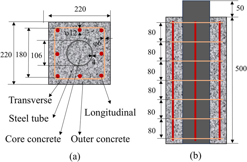
Figure 4. Schematic diagram and dimensions of test piece. (a) Top plan, (b) Front view.

Table 1

Table 1. The mix ratio of concrete (kg/m³).

Table 2

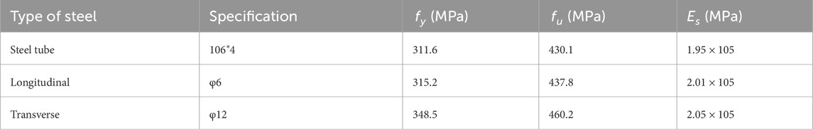
Table 2. The properties of steel.

For the push-out test, a 1,500 kN low electro-hydraulic servo actuator was selected, and a displacement control was used for loading, with a loading rate control of 0.005 mm/s. As shown in Figure 5, the test setup mainly consisted of an actuator, a load plate, a steel plate, a rigid base and four displacement gauges. The size of the steel pad plate is 340 mm × 340 mm × 30 mm, and a circular hole with a diameter of 135 mm is opened in the center so that the steel pipe can pass through the circular hole during the push-out test. Four displacement gauges were placed at the four corners of the loading plate to check whether the specimen was under axial compression.

Figure 5

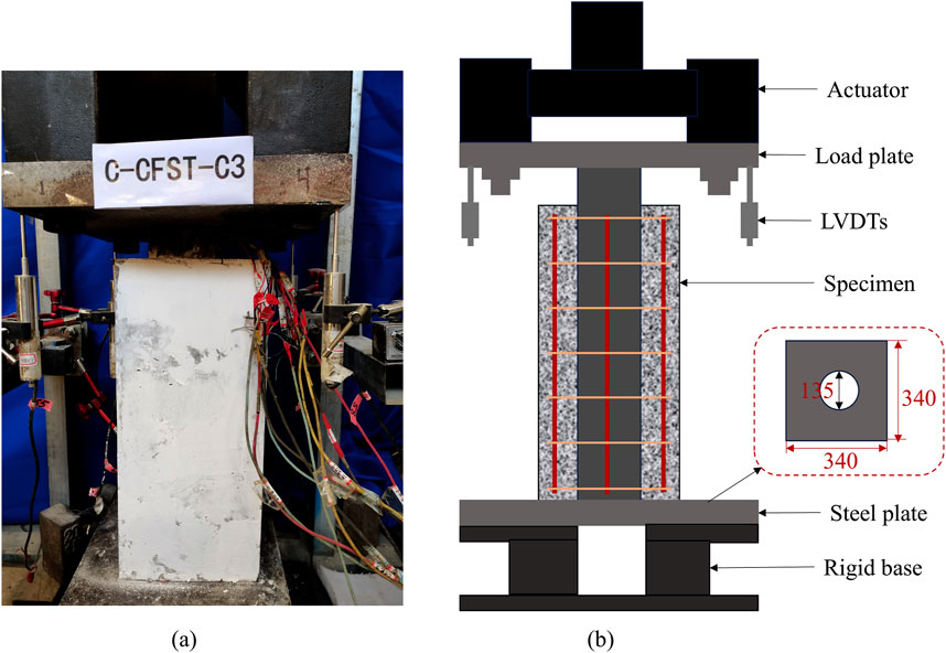
Figure 5. Schematic diagram of the loading device. (a) Testing photo, (b) Diogram of loading device.

In order to utilize the acoustic characteristics to identify the cracks, we conducted the percussion tests on the specimens at different crack widths. The equipment for the percussion test mainly consisted of a Signal Acquisition Instrument (INV3062SV; COINV Orient Institute), a computer, a sound pressure sensor (INV9204; COINV Orient Institute), and a percussion hammer (INV9313; COINV Orient Institute) as shown in Figure 6.

Figure 6

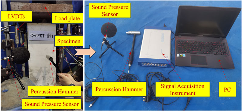
Figure 6. Percussion signal acquisition device.

The test procedure is as follows: i) First, slowly apply pressure to the specimen to 30 kN, at this time the specimen is not cracked, the loading displacement is recorded as 0 cm, to keep the stress unchanged, the specimen is continuously percussed for 150 times and the sound data is recorded, and the tapping point is set in the center of an unpressurized surface. ii) Then, continue to pressurize until the displacement reaches 5 cm (at this time the concrete has cracked). iii)Stop loading and slowly decrease the pressure to 30 kN. iv) Use the crack width meter to measure the cracking width of the cracked surface of the specimen along the length direction of the center line. v) At the left position on the center line and not more than 1 cm away from the crack, perform 150 consecutive taps and record the sound data. vi) Continue loading until the displacements reached 10 cm, 15 cm, 20 cm and 25 cm respectively (the final displacements of both specimens at the time of failure were more than 30 cm), and then repeat the operations of steps iii) to v) in turn. Finally, the percussion sound data of two specimens at six different crack widths were obtained. It should be noted that the results of the literature (Chen et al., 2022) have shown that the structural surface stiffness affects the variation of the tapping sound, and for this study, when the tapping position is changed, due to the inhomogeneity of the cracks, etc. Will lead to the change of the indicated stiffness of the tapping position, and thus it can be expected that the identification results of the model will be decreased, so that the repetition of the tapping position will not be repeated in this study. The photographs of the cracks of specimen A under different loading displacements are given in Figure 7. Table 3 summarizes the crack widths in the middle of the 2 specimens under different loading displacements.

Figure 7

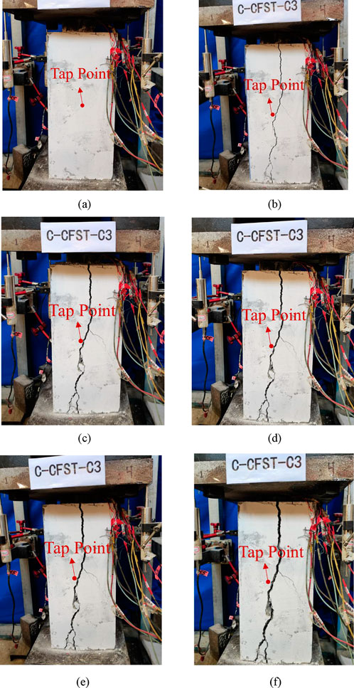
Figure 7. Photographs of cracks under different loading displacements: (a) 0 cm; (b) 5 cm; (c) 10 cm; (d) 15 cm; (e) 20 cm; (f) 25 cm.

Table 3

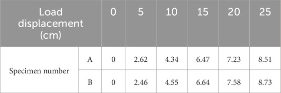
Table 3. Crack widths in the middle of concrete under different loading displacements (mm).

4.2 Sound data acquisition and pre-processing

The deep learning process usually requires a larger number of data points for training to prevent the model from overfitting or poor classification performance. Therefore, many scholars use data enhancement methods to expand the dataset needed for training (Chen et al., 2022). However, for the same data sample, they usually adopt only one technique for processing, failing to fully consider the diversity of data (Wang et al., 2021a). For this reason, this paper adopts a combination of multiple enhancement techniques to enhance the concrete percussion sound data, and the number of data enhancement is two times in order to fully consider the diversity and sufficiency of the data. In this case, the first enhancement is done using shift technique + change volume technique + stretch technique while the second enhancement is done using shift technique + change volume technique + zoom technique. As can be seen from Section 4.1, a total of 900 sound data were collected for each specimen, and after two data enhancements, the amount of data was tripled, i.e., 2,700 data points were obtained for each specimen, which was able to satisfy the training requirements of the model to a greater extent. The principles of the four data enhancement techniques are described as follows: i) Shift technique refers to removing a segment X (n₁:n₂) of the original signal X(n) and inserting it into position n₃ to realize the movement of the segment. ii) Change volume technique refers to altering the amplitude value of the original signal X(n), with the mathematical expression Y(n) = G*X(n), where G is the gain factor, and when G > 1, it is an amplified signal, and when 0 < G < 1, it is an attenuated signal. iii) The stretch technique is a technique to change the playback speed of an audio signal without altering its pitch, by choosing a stretching factor β (usually greater than 1.0), it can make the audio signal faster, and its mathematical expression is Y(n) = G*X (n/β). vi) The Zoom technique is the opposite technique to Stretch, simply set β to a value less than 1.0.

Figure 8 shows the data augmentation process for the percussion sound of specimen A. The sound signal was first cut into 0.02 s segments from the continuous original signal, and each segment had the same sampling frequency as the original audio.

Figure 8

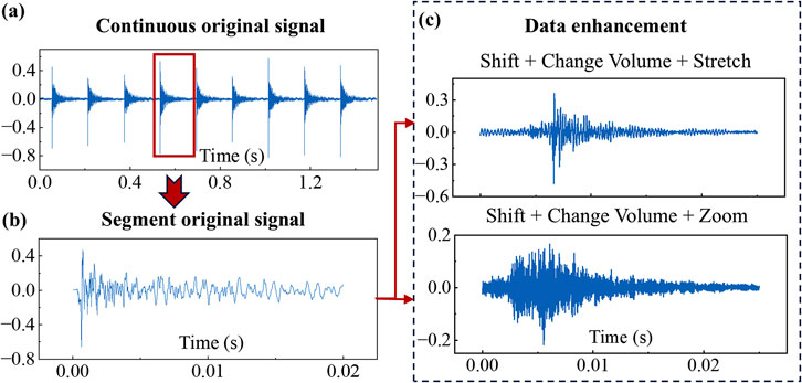
Figure 8. Example of data enhancement of the tapping sound of specimen A: (a) Continuous original signal; (b) Segment original signal; (c) Data enhancement.

After completing the data enhancement, MFCC extraction is required, and the MFCC results corresponding to six different crack widths are shown in Figure 9. The horizontal coordinate in the figure is the time and the vertical coordinate is the frequency. It can be observed that although the MFCC plots correspond to different crack widths, they all have a small number of more prominent regions, and there is a large overall similarity, making it difficult to distinguish them directly. Specifically, in Figure 9a, when the crack width is 0 mm, there are mainly three distinct regions in the MFCC mapping, which are located in the frequency intervals of 0 Hz∼1,000 Hz, 1,000 Hz∼2,500 Hz, and 8,000 Hz∼10,000 Hz, respectively. In Figure 9b, when a crack of 2.62 mm occurs, the corresponding MFCC map has one more obvious region between 450 Hz and 5,000 Hz, in addition, the frequency interval of the original third obvious region has been expanded, from 8,000 Hz∼10,000 Hz–5,100 Hz ∼11,000 Hz. In Figure 9c, when the crack is enlarged to 4.34 mm, the number of distinct regions and the frequency interval of the corresponding MFCC map are close to those of the MFCC map for 2.62 mm, but its color becomes lighter in comparison. In Figure 9d, when the crack further increases to 6.47 mm, the frequency interval from 450 Hz to 5,000 Hz becomes less obvious, and the original obvious region from 5,100 Hz to 11,000 Hz is also compressed. In Figure 9e, when the crack increases to 7.23 mm, compared with 6.47 mm, only part of the 5,100 Hz ∼ 11,000 Hz region is observed to become darker in color, and the other changes cannot be effectively identified by the naked eye. In Figure 9f, when the crack increases to 8.51 mm, compared with 7.23 mm, a small degree of compression occurs in the apparent region of 5,100 Hz ∼11,000 Hz, and a section of color deepening is found in the frequency interval of 1,000 Hz ∼ 2,500 Hz, with the duration of 0 s ∼ 0.035 s. In particular, the feature areas in the maps are so large that it is difficult to establish a complex mapping relationship between the large feature maps and crack widths by manual generalization. A similar phenomenon was found when specimen B was analyzed. Therefore, a deep learning network with strong feature learning capability is required for identification.

Figure 9

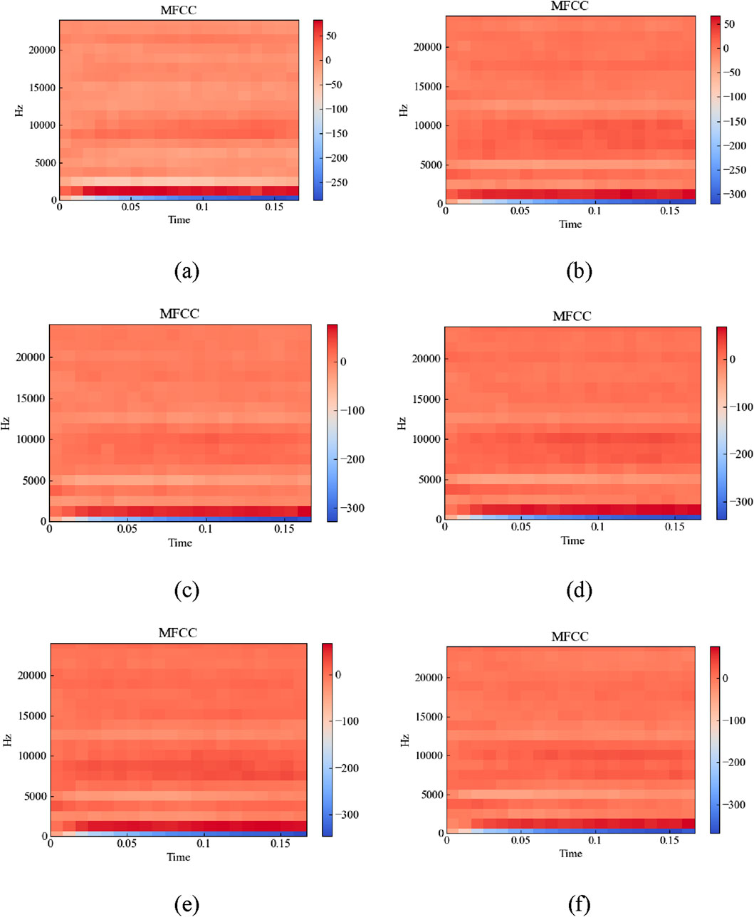
Figure 9. MFCC for different crack widths: (a) 0 cm; (b) 2.6 cm; (c) 4.3 cm; (d)6.4 cm; (e) 7.2 cm; (f) 8.5 cm.

For the data at different widths, this paper is divided into training, validation, and test sets in the ratio of 4:1:5, with a batch size of 32 and a learning rate of 0.006. For specimen A, the labels corresponding to crack widths of 0 mm, 2.62 mm, 4.34 mm, 6.47 mm, 7.23 mm and 8.51 mm were set to CW0, CW2.62, CW4.33, CW6.47, CW7.23 and CW8.51, respectively. Similarly, specimen B was similarly labeled using the same approach. The computer configuration used for the experiment is: CPU is Intel(R) Core(TM) i9-9,900X at 3.50 GHz; the graphics card is NVIDIA TITAN Xp made by NVIDIA; the development environment is CUDA10.2, and the network framework is Pytorch1.11.

4.3 Effect of different sample frame lengths

In this subsection, we evaluate the effect of different input sample frame lengths on the training performance of the model by setting the input sample frame lengths to 128,256,512,1024 and 2048, respectively, and selecting the optimal frame length by analyzing the accuracy and loss. Taking specimen B as an example, Figure 10 gives the curve of the influence of different input sample frame lengths on the accuracy and loss of the model validation process. It can be seen that, with the increase of epoch, the validation accuracy under different frame lengths first increases, and then all of them show a significant decrease at epoch = 5, and then continue to increase, and finally fluctuate up and down around 100%. The corresponding verification loss curve is the opposite. As the epoch increases, the validation loss curve first gradually decreases, then abruptly increases at epoch = 5, and then continues to decrease to near 0. It is worth noting that when the frame length is 1,024, the verification accuracy curve converges faster, with higher accuracy and smaller final loss values. Therefore, in the subsequent calculation process, we set the frame length of MFCC to 1,024 uniformly.

Figure 10

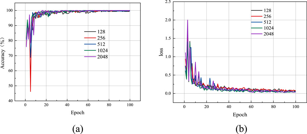
Figure 10. Effect of frame lengths on model validation accuracy and validation loss. (a) Verification accuracy, (b) Verification loss.

4.4 Ablation experiments

In order to explore the performance improvement effect on the CNN model brought about by the optimization approach using the transfer learning and SENet attention mechanism, the ablation tests were carried out using the data of specimen A as an example, and the results are shown in Table 4. In the table, No. 1 indicates the original CNN model, No. 2 indicates the method of transfer learning introduced based on the CNN model, No. 3 indicates the introduction of SENet attention based on the CNN model, and No. 4 indicates the method proposed in this paper, i.e., both transfer learning and SENet attention are introduced based on CNN model.

Table 4

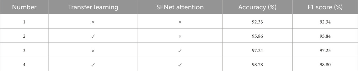
Table 4. Ablation tests of the TSCNN model.

As can be seen from Table 4, the introduction of transfer learning in the CNN model improves the accuracy of the model by 3.53 percentage points and the F1 score by 3.5 percentage points. This indicates that the transfer learning technique initializes the weights of the model through pre-training, which can effectively improve the training starting point of the model and thus improve the accuracy of recognition, which is consistent with the findings of the existing study (Gupta et al., 2021). After embedding SENet attention into the basic unit of CNN, the accuracy and F1 score of the model are both improved to 4.91 percentage points. This is because SENet attention enhances the model’s focus on important features of the MFCC input graph, while suppressing the interference of useless features on the recognition performance. And after combining the improvements of transfer learning and SENet attention, the performance of the CNN is greatly improved, with accuracy and F1 scores of 98.78% and 98.80%, respectively, which are 6.45 percentage points and 6.46 percentage points respectively compared with the original CNN model. This indicates that the improved method based on transfer learning and SENet attention is efficient and able to improve the accuracy of the model in recognizing different degrees of cracking in concrete.

4.5 Effect of different models

In order to verify the superiority of the proposed method in concrete crack recognition, it is compared with Resnet18 (Liu et al., 2023), random forest (RF) (Belgiu and Drăguţ, 2016), and long short-term memory (LSTM) network (Song et al., 2020) respectively, and the results are shown in Figure 11. It can be seen that the recognition accuracy of both Resnet18 and RF models is not high. For specimen A and specimen B, the recognition accuracies obtained by the Resnet18 model are only 82.54% and 80.73%, respectively, while the RF model is only 78.52% and 82.15%, respectively. On the other hand, the recognition accuracy of the LSTM model is relatively higher, with the accuracy of the two specimens corresponding to 90.94% and 91.47%, respectively. This indicates that the feature learning ability of LSTM for MFCC maps with different crack widths is higher than the previous two models, but the accuracy is still not very satisfactory. The TSCNN model proposed in this paper, based on CNN, applies the transfer learning technique to improve the starting point of model training and introduces the SENet attention mechanism, which enables the model to enhance the focus on important features and suppress the interference of useless features, thus effectively improving the recognition accuracy of crack width. For specimen A and specimen B, the proposed models achieved 98.78% and 98.45%, respectively. Overall, the average recognition accuracies of the four different models are ranked as TSCNN > LSTM > Resnet18>RF. In addition, comparing the magnitude of change in the accuracy of the four models between two specimens, it is found that the magnitude of change is 1.81% for Resnet18, 3.63% for RF, 0.53% for LSTM, and 0.33% for TSCNN, which suggests that TSCNN is the smallest variation among the four models. Therefore, it can be assumed that the TSCNN model has better stability. The combined results show that the method proposed in this paper can effectively identify the crack width of concrete, and its performance and stability are better than other traditional methods.

Figure 11

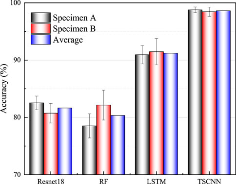
Figure 11. The recognition accuracy of different models.

4.6 Effect of different signal-to-noise ratios (SNR)

Due to the field inspection process, the percussion sound signal is easily affected by external noise, which may weaken the performance of the crack width recognition model. Therefore, in order to verify the noise robustness of the proposed method, noise is added to the test data for testing in this paper. As shown in Equation 17, Gaussian white noise is added to the test data to achieve the corresponding SNR (Wang and Song, 2021):

$\text{SNR}=10{\log }_{10}\left(\frac{A_0^2}{A_1^2}\right)(17)$

Where, $A_0$ denotes the amplitude of the original signal, and $A_1$ denotes the amplitude of the noise. The signal-to-noise ratio ranges from -9db to 6 db with a spacing of 3 db. The process of adding noise with a SNR of 6 db is given in Figure 12.

Figure 12

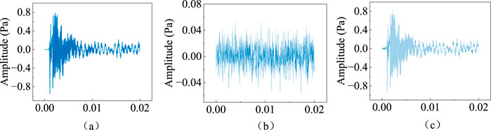
Figure 12. The process of adding noise with a SNR of 6 db: (a) original signal; (b) white noise; (c) synthesized signal (SNR = 6 db).

It should be noted that, since the technique proposed in this study is still at the stage of indoor exploration and fails to comprehensively consider the complex noise environment in a real site, Gaussian white noise is analyzed in this paper as a commonly used tool, and other types of noises, such as mechanical and electrical noises, are not included in the discussion for the time being. The recognition results of different models at different SNR are shown in Figure 13. It can be observed that for specimen A, in the noise environment of -9db, the recognition accuracies of all the models are significantly decreased, which is lower than 65%. During the increase of SNR from -6 db to 6db, the recognition accuracies of all models show an overall increasing trend, but only the accuracy of the proposed TSCNN model is always higher than 90%, and the accuracies obtained by the other models are basically below 90%. In the noisy environment with SNR equal to 6 db, i.e., the group with the highest recognition performance, the accuracy of the TSCNN model increased by 17.09%, 22.1% and 6.77% compared to Resnet18, RF and LSTM, respectively. For specimen B, the trend of the four models is basically similar to that of specimen A, but the overall accuracy is slightly lower. However, the accuracy of the TSCNN model for crack width identification is still maintained at 85%–98% under the noise environment of -6db–6 db. In summary, the proposed TSCNN model has a better denoising ability than other models in the noise environment with SNR of -6db∼6 db.

Figure 13

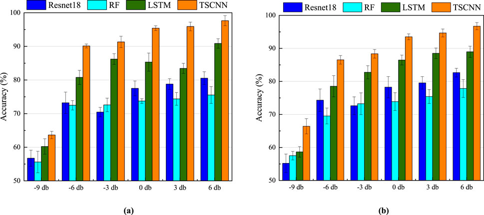
Figure 13. Accuracy of different models at different SNR: (a) Specimen A; (b) Specimen B.

4.7 Visualization

In order to gain insight into the feature learning ability of the SCNN model in different noise environments, the t-SNE technique (Kobak and Berens, 2019) is used to visualize the recognition results. The common patterns of clustering in the t-SNE technique are divided into three main types: clear boundaries between different categories, fuzzy boundaries between different categories and random distribution of different categories. The first pattern usually indicates that the model has good recognition accuracy for different labeled categories and is rarely misclassified. The second pattern corresponds to different recognition accuracies depending on the degree of boundary blurring, and the more blurred labels, the worse the accuracy. The third pattern implies that the model is basically invalid and cannot discriminate different label categories effectively. Figure 14 shows the visualization results of TSCNN in specimen A. It can be seen that there are obvious boundaries between different labels under other SNR noises except for -9db, which clearly separates different labels, which corresponds to a recognition accuracy higher than 90% in Section 4.5. The visualization results for specimen B are shown in Figure 15. It can be observed that specimen B performs similarly to specimen A in a -9bd SNR environment, with more serious mixing between different labels, indicating that the performance of the TSCNN model is not so good at low SNR. Although there is a small range of interleaving phenomenon of some labels in -6bd SNR environment, it does not affect the recognition results. The results show that the proposed TSCNN method has good feature learning ability for MFCC maps corresponding to different crack widths, and can realize high-precision recognition of crack widths in high signal-to-noise ratio (-6db∼6 db) noise environments.

Figure 14

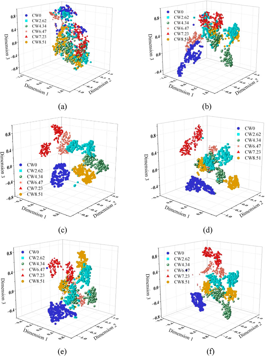
Figure 14. Visualization of TSCNN in Specimen A. (a) −9 db, (b) −6 db, (c) −3 db, (d) 0 db, (e) 3 db, (f) 6 db.

Figure 15

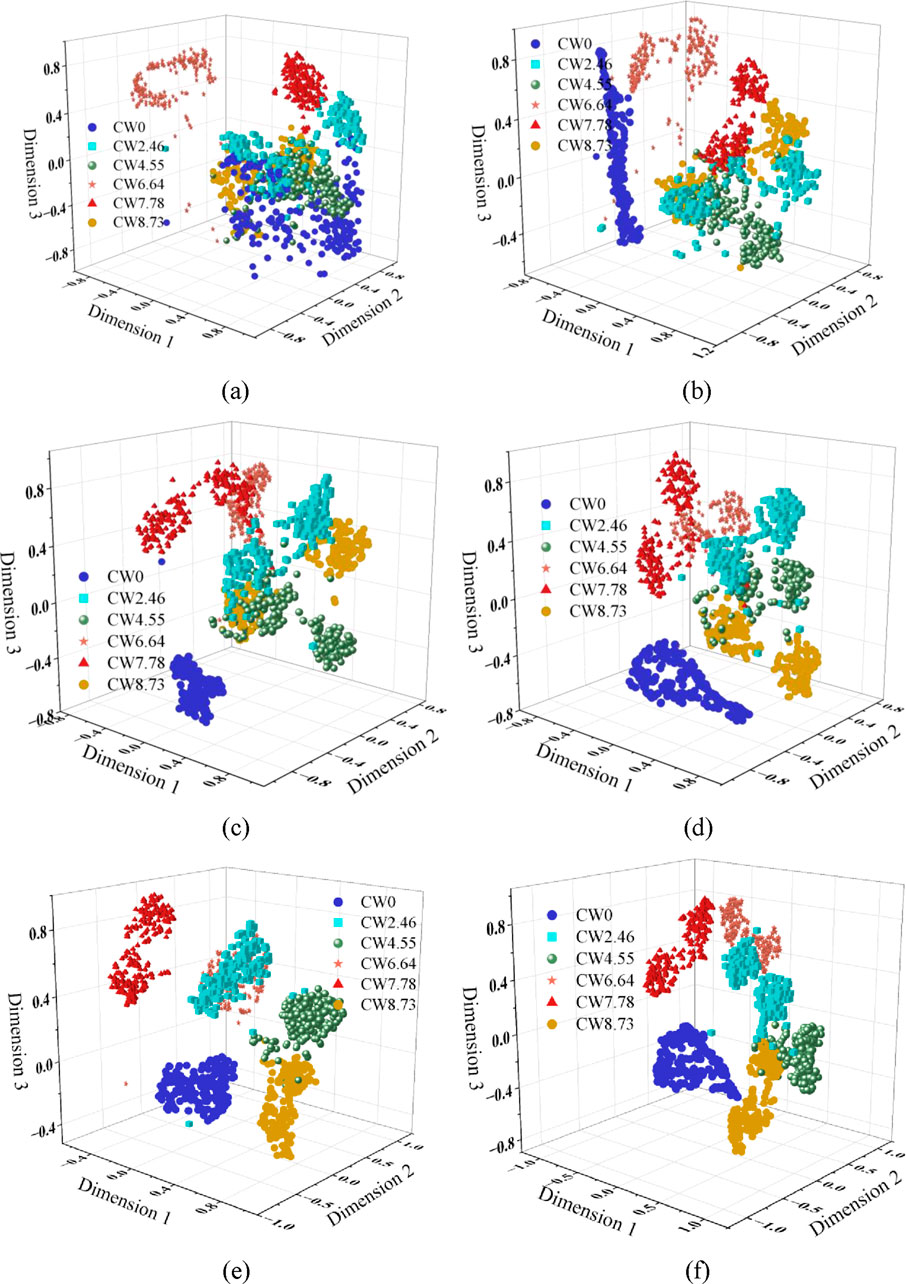
Figure 15. Visualization of TSCNN in Specimen B. (a) −9 db, (b) −6 db, (c) −3 db, (d) 0 db, (e) 3 db, (f) 6 db.

5 Conclusion

In this paper, an innovative method combining MFCC and improved CNN based on Percussion Detection technique is proposed to identify the crack width of concrete. The method is a fast and effective means of detection as it does not require the coupling of installed sensors. A series of indoor exploratory tests were conducted using the proposed method to demonstrate its effectiveness and accuracy. The following main conclusions are obtained:

(1) The method of using the combined enhancement technique to enhance the percussion sound signal can effectively solve the problems of insufficient data samples and data monotony, which helps to improve the generalization ability of the model.

(2) A crack width recognition model based on an improved CNN network is proposed. The method is pre-trained by the transfer learning technique, which effectively improves the training starting point of the CNN model; the embedded SENet attention enables the CNN model to focus on important features, which in turn improves the recognition performance.

(3) The proposed model is accurate and effective. The proposed model obtains an average recognition accuracy of 98.62% with a variation of only 0.33% in two different specimen tapping tests, which is more accurate and more stable than other conventional models (Resnet18, RF and LSTM).

(4) In a high signal-to-noise ratio (-6db∼6 db) environment, the proposed model shows good noise robustness and the accuracy is maintained between 85% and 98%. Therefore, it can be concluded that the method based on percussion with improved CNN proposed in this paper has a large potential in the future field detection of concrete cracks.

The study in this paper verifies the effectiveness of the proposed method in terms of concrete cracking width. However, there are still some shortcomings: i) it fails to adequately consider the impact of additional structural parameters and quantities on the identification results, such as structural dimensions, reinforcement ratios, surface cleanliness, etc., while the conclusions do not take into account field data or environmental variability (e.g., ambient noise). ii) Although the method in this paper validates its effectiveness in surface crack identification, there is still no discussion on the depth of cracks, sensor positioning, and variation of structure variability. In the follow-up research work, we will design tests with different structural parameters to verify the generalization ability of the model on more specimens with different parameters rejected.

Data availability statement

The raw data supporting the conclusions of this article will be made available by the authors, without undue reservation.

Author contributions

CG: Conceptualization, Resources, Software, Supervision, Writing – original draft. YQ: Data curation, Formal Analysis, Methodology, Writing – original draft. KX: Writing – original draft, Writing – review and editing. ZL: Software, Visualization, Writing – review and editing.

Funding

The author(s) declare that no financial support was received for the research and/or publication of this article.

Conflict of interest

Author ZL was employed by Guangxi Communications Investment Group Co., Ltd. and Nanning Expressway Operation Co., Ltd.

The remaining authors declare that the research was conducted in the absence of any commercial or financial relationships that could be construed as a potential conflict of interest.

Generative AI statement

The author(s) declare that no Generative AI was used in the creation of this manuscript.

Publisher’s note

All claims expressed in this article are solely those of the authors and do not necessarily represent those of their affiliated organizations, or those of the publisher, the editors and the reviewers. Any product that may be evaluated in this article, or claim that may be made by its manufacturer, is not guaranteed or endorsed by the publisher.

References

Belgiu, M., and Drăguţ, L. (2016). Random forest in remote sensing: a review of applications and future directions. ISPRS J. photogrammetry remote Sens. 114, 24–31. doi:10.1016/j.isprsjprs.2016.01.011

CrossRef Full Text | Google Scholar

Cawley, P., and Adams, R. (1988). The mechanics of the coin-tap method of non-destructive testing. J. sound Vib. 122 (2), 299–316. doi:10.1016/S0022-460X(88)80356-0

CrossRef Full Text | Google Scholar

Chen, D., and Mahadevan, S. (2008). Chloride-induced reinforcement corrosion and concrete cracking simulation. Cem. Concr. Compos. 30 (3), 227–238. doi:10.1016/j.cemconcomp.2006.10.007

CrossRef Full Text | Google Scholar

Chen, D., Montano, V., Huo, L., Fan, S., and Song, G. (2020a). Detection of subsurface voids in concrete-filled steel tubular (CFST) structure using percussion approach. Constr. Build. Mater. 262, 119761. doi:10.1016/j.conbuildmat.2020.119761

CrossRef Full Text | Google Scholar

Chen, D., Montano, V., Huo, L., and Song, G. (2020b). Depth detection of subsurface voids in concrete-filled steel tubular (CFST) structure using percussion and decision tree. Measurement 163, 107869. doi:10.1016/j.measurement.2020.107869

CrossRef Full Text | Google Scholar

Chen, D., Shen, Z., Huo, L., and Narazaki, Y. (2023). Percussion-based quasi real-time void detection for concrete-filled steel tubular structures using dense learned features. Eng. Struct. 274, 115197. doi:10.1016/j.engstruct.2022.115197

CrossRef Full Text | Google Scholar

Chen, L., Xiong, H., Sang, X., Yuan, C., Li, X., and Kong, Q. (2022). An innovative deep neural network–based approach for internal cavity detection of timber columns using percussion sound. Struct. Health Monit. 21 (3), 1251–1265. doi:10.1177/14759217211028524

CrossRef Full Text | Google Scholar

Goszczyńska, B., Świt, G., Trąmpczyński, W., Krampikowska, A., Tworzewska, J., and Tworzewski, P. (2012). Experimental validation of concrete crack identification and location with acoustic emission method. Archives Civ. Mech. Eng. 12, 23–28. doi:10.1016/j.acme.2012.03.004

CrossRef Full Text | Google Scholar

Gowripalan, N., Sirivivatnanon, V., and Lim, C. (2000). Chloride diffusivity of concrete cracked in flexure. Cem. Concr. Res. 30 (5), 725–730. doi:10.1016/s0008-8846(00)00216-7

CrossRef Full Text | Google Scholar

Gupta, S., Agrawal, M., and Deepak, D. (2021). Gammatonegram based triple classification of lung sounds using deep convolutional neural network with transfer learning. Biomed. Signal Process. Control 70, 102947. doi:10.1016/j.bspc.2021.102947

CrossRef Full Text | Google Scholar

Hsiao, C., Cheng, C.-C., Liou, T., and Juang, Y. (2008). Detecting flaws in concrete blocks using the impact-echo method. NDT and E Int. 41 (2), 98–107. doi:10.1016/j.ndteint.2007.08.008

CrossRef Full Text | Google Scholar

Kaufmann, W., and Marti, P. (1998). Structural concrete: cracked membrane model. J. Struct. Eng. 124 (12), 1467–1475. doi:10.1061/(ASCE)0733-9445(1998)124:12(1467)

CrossRef Full Text | Google Scholar

Kim, B., and Cho, S. (2018). Automated vision-based detection of cracks on concrete surfaces using a deep learning technique. Sensors 18 (10), 3452. doi:10.3390/s18103452

PubMed Abstract | CrossRef Full Text | Google Scholar

Kobak, D., and Berens, P. (2019). The art of using t-SNE for single-cell transcriptomics. Nat. Commun. 10 (1), 5416. doi:10.1038/s41467-019-13056-x

PubMed Abstract | CrossRef Full Text | Google Scholar

Koch, C., Georgieva, K., Kasireddy, V., Akinci, B., and Fieguth, P. (2015). A review on computer vision based defect detection and condition assessment of concrete and asphalt civil infrastructure. Adv. Eng. Inf. 29 (2), 196–210. doi:10.1016/j.aei.2015.01.008

CrossRef Full Text | Google Scholar

Kong, Q., Zhu, J., Ho, S. C. M., and Song, G. (2018). Tapping and listening: a new approach to bolt looseness monitoring. Smart Mater. Struct. 27 (7), 07LT02. doi:10.1088/1361-665x/aac962

CrossRef Full Text | Google Scholar

Kubojima, Y., Sonoda, S., and Kato, H. (2018). Practical techniques for the vibration method with additional mass: bending vibration generated by tapping cross section. J. wood Sci. 64 (1), 16–22. doi:10.1007/s10086-017-1676-6

CrossRef Full Text | Google Scholar

Liu, L., Fan, K., and Yang, M. (2023). Federated learning: a deep learning model based on resnet18 dual path for lung nodule detection. Multimedia Tools Appl. 82 (11), 17437–17450. doi:10.1007/s11042-022-14107-0

CrossRef Full Text | Google Scholar

Matallah, M., and La Borderie, C. (2009). Inelasticity–damage-based model for numerical modeling of concrete cracking. Eng. Fract. Mech. 76 (8), 1087–1108. doi:10.1016/j.engfracmech.2009.01.020

CrossRef Full Text | Google Scholar

Murty, K. S. R., and Yegnanarayana, B. (2005). Combining evidence from residual phase and MFCC features for speaker recognition. IEEE signal Process. Lett. 13 (1), 52–55. doi:10.1109/LSP.2005.860538

CrossRef Full Text | Google Scholar

Ohno, K., and Ohtsu, M. (2010). Crack classification in concrete based on acoustic emission. Constr. Build. Mater. 24 (12), 2339–2346. doi:10.1016/j.conbuildmat.2010.05.004

CrossRef Full Text | Google Scholar

Pahlavan, L., Zhang, F., Blacquière, G., Yang, Y., and Hordijk, D. (2018). Interaction of ultrasonic waves with partially-closed cracks in concrete structures. Constr. Build. Mater. 167, 899–906. doi:10.1016/j.conbuildmat.2018.02.098

CrossRef Full Text | Google Scholar

Rasol, M. A., Pérez-Gracia, V., Solla, M., Pais, J. C., Fernandes, F. M., and Santos, C. (2020). An experimental and numerical approach to combine Ground Penetrating Radar and computational modeling for the identification of early cracking in cement concrete pavements. Ndt and E Int. 115, 102293. doi:10.1016/j.ndteint.2020.102293

CrossRef Full Text | Google Scholar

Sirca, J. , G. F., and Adeli, H. (2018). Infrared thermography for detecting defects in concrete structures. J. Civ. Eng. Manag. 24 (7), 508–515. doi:10.3846/jcem.2018.6186

CrossRef Full Text | Google Scholar

Song, X., Liu, Y., Xue, L., Wang, J., Zhang, J., Wang, J., et al. (2020). Time-series well performance prediction based on Long Short-Term Memory (LSTM) neural network model. J. Petroleum Sci. Eng. 186, 106682. doi:10.1016/j.petrol.2019.106682

CrossRef Full Text | Google Scholar

Tashan, J., and Al-Mahaidi, R. (2014). Detection of cracks in concrete strengthened with CFRP systems using infra-red thermography. Compos. Part B Eng. 64, 116–125. doi:10.1016/j.compositesb.2014.04.011

CrossRef Full Text | Google Scholar

Tosti, F., and Ferrante, C. (2020). Using ground penetrating radar methods to investigate reinforced concrete structures. Surv. Geophys. 41 (3), 485–530. doi:10.1007/s10712-019-09565-5

CrossRef Full Text | Google Scholar

Wang, F., Mobiny, A., Van Nguyen, H., and Song, G. (2021a). If structure can exclaim: a novel robotic-assisted percussion method for spatial bolt-ball joint looseness detection. Struct. Health Monit. 20 (4), 1597–1608. doi:10.1177/1475921720923147

CrossRef Full Text | Google Scholar

Wang, F., and Song, G. (2020). Looseness detection in cup-lock scaffolds using percussion-based method. Automation Constr. 118, 103266. doi:10.1016/j.autcon.2020.103266

CrossRef Full Text | Google Scholar

Wang, F., and Song, G. (2021). A novel percussion-based method for multi-bolt looseness detection using one-dimensional memory augmented convolutional long short-term memory networks. Mech. Syst. Signal Process. 161, 107955. doi:10.1016/j.ymssp.2021.107955

CrossRef Full Text | Google Scholar

Wang, F., Song, G., and Mo, Y. L. (2021b). Shear loading detection of through bolts in bridge structures using a percussion-based one-dimensional memory-augmented convolutional neural network. Computer-Aided Civ. Infrastructure Eng. 36 (3), 289–301. doi:10.1111/mice.12602

CrossRef Full Text | Google Scholar

Wang, H., Xu, J., Yan, R., and Gao, R. X. (2019). A new intelligent bearing fault diagnosis method using SDP representation and SE-CNN. IEEE Trans. Instrum. Meas. 69 (5), 2377–2389. doi:10.1109/TIM.2019.2956332

CrossRef Full Text | Google Scholar

Yang, H., Liu, J., Mei, G., Yang, D., Deng, X., and Duan, C. (2023). Research on real-time detection method of rail corrugation based on improved ShuffleNet V2. Eng. Appl. Artif. Intell. 126, 106825. doi:10.1016/j.engappai.2023.106825

CrossRef Full Text | Google Scholar

Yang, Z., and Huo, L. (2022). Bolt preload monitoring based on percussion sound signal and convolutional neural network (CNN). Nondestruct. Test. Eval. 37 (4), 464–481. doi:10.1080/10589759.2022.2030735

CrossRef Full Text | Google Scholar

Yao, P., Wang, J., Zhang, F., Li, W., Lv, S., Jiang, M., et al. (2022). Intelligent rolling bearing imbalanced fault diagnosis based on mel-frequency cepstrum coefficient and convolutional neural networks. Measurement 205, 112143. doi:10.1016/j.measurement.2022.112143

CrossRef Full Text | Google Scholar

Zheng, L., Cheng, H., Huo, L., and Song, G. (2019). Monitor concrete moisture level using percussion and machine learning. Constr. Build. Mater. 229, 117077. doi:10.1016/j.conbuildmat.2019.117077

CrossRef Full Text | Google Scholar