Unsettling the settled: simple musings on the complex climatic system

Our revisit of fundamental issues of climate challenges the notion and term of the “greenhouse effect”, and attempts a scientific reevaluation using minimal assumptions, such as Newton’s laws, maximum entropy and gas spectroscopy. It replaces terms like “greenhouse gas” with “radiatively active gas” (RAG) and “greenhouse effect” with “atmospheric radiative effect” (ARE). While ARE exists in several planets’ atmospheres, on Earth it is primarily driven by water vapor and clouds, with CO₂ playing a minor role (especially anthropogenic CO₂ which represents 4% of total emissions). Equilibrium thermodynamics, via entropy maximization or molecular collision simulation, leads to an isothermal atmosphere at about 250 K (the average temperature of the troposphere and stratosphere) irrespective of RAG presence or not. It is the troposphere’s 6.5 K/km temperature gradient (lapse rate), partly shaped by moist adiabatic processes, that drives the atmosphere away from this equilibrium and warms the surface to about 288 K on average, with ARE (mainly water vapor and clouds) contributing to the warming, but only when this gradient exists. The temperature gradient varies spatially and temporally and, since 1950, has weakened in the tropics and grown in the polar areas, resulting in a decrease of the surface equator-to-pole gradient, as expected in global warming conditions.

1 Introduction

Do we live in a greenhouse? Most people would give an affirmative reply given the enormous campaign to promote the climate initiatives that are founded on the concepts of greenhouse gases (GHG) and greenhouse effect (GHE). Systematic searches in Google Books (https://books.google.com/ngrams/) and Internet Archive (https://archive.org/) show that, while the term ‘greenhouse’ is old (already appearing in the 18th century with its literal meaning), the terms GHG and GHE are newer. Following Poynting (1907) who used the term GHE for planetary atmospheres (even though he was criticized by Very, 1908; see Supplementary Appendix SA), the term GHE as it relates to planetary atmospheres was popularized in 1960s by NASA (Samuelson, 1965; Wildt, 1965). Since the late 1970s, however, the usage of GHE has changed to closely associate it with carbon dioxide (CO₂) and its emission into the atmosphere from the burning of fossil fuels, but also to imply that this causes disastrous effects on climate, economy and every aspect of life (Murray, 1979; Bernard Jr, 1980; EXXON, 1982; Gribbin, 1982; Barth and Titus, 1984; U.S. House of Representatives, 1984; Bolin et al., 1986; Gay, 1986).

From a scientific perspective, clarity in terminology is essential (cf. the Aristotelian notion of sapheneia; Koutsoyiannis, 2024a). In strict scientific terms, the reply to the question whether we live in a greenhouse is negative: The Earth’s atmosphere does not function like a greenhouse. A simple revisit of the definition of a greenhouse (a structure that is designed to regulate the temperature and humidity of the environment inside) suffices to see this, even though effects such as those that the term GHE purports to describe are present on Earth, as well as on other planets in the solar system with atmospheres (see section 3.2). Hence, the term GHE can be misleading as further explained in Supplementary Appendix SA.

For scientific clarity and accuracy, we propose replacing the term GHG with radiatively active gas (RAG), comprising water vapor (WV) and non-condensing radiatively active gases (NC-RAGs). We also propose replacing the term GHE with atmospheric radiative effect (ARE). ARE is the influence of RAGs on the energy balance in the atmosphere by absorbing, emitting, and scattering radiation across both shortwave (SW) and longwave (LW) spectra. These processes influence the flow of energy between the Earth’s surface, the atmosphere, and space. While the term GHE is often associated primarily with heat-trapping, ARE explicitly recognizes all radiative interactions in the atmosphere. It avoids the misleading analogy of a greenhouse and is more applicable to a scientific framework that considers both SW and LW radiation. For the reader’s convenience, these acronyms are listed and explained in Table 1, along with all other abbreviations used in this paper.

Table 1

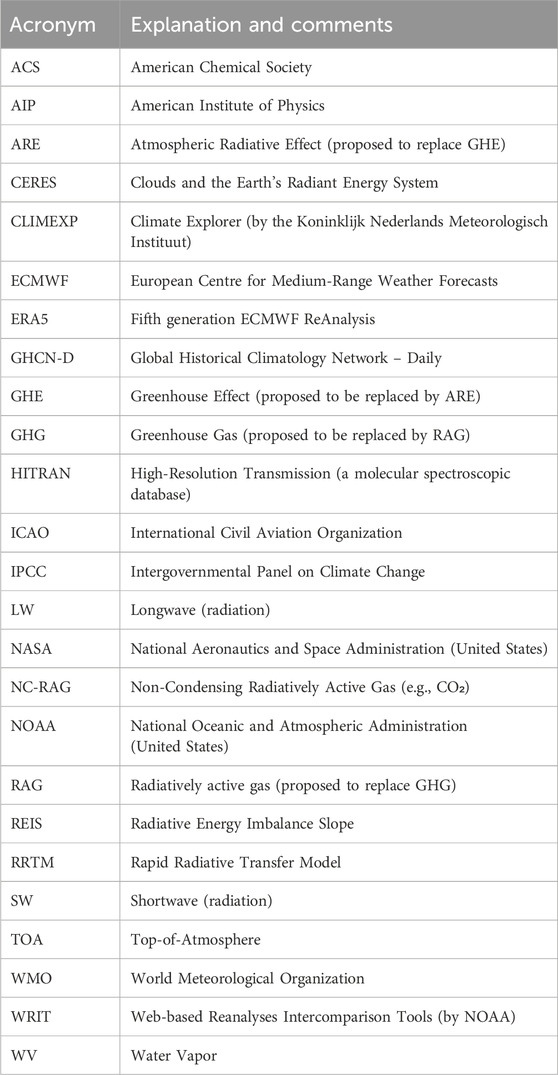
Table 1. List of acronyms used in this paper.

Notably, WV and clouds (for which WV is responsible) dominate ARE, while CO₂ contributes only 4%–5% to it (Koutsoyiannis, 2024b). Also, anthropogenic CO₂ emissions are only 4% of the total, with the vast majority (96%) being natural (Koutsoyiannis et al., 2023). Additionally, evidence suggests that changes in temperature precede those in CO₂ concentration, thus challenging the assumption that CO₂ drives temperature (Koutsoyiannis et al., 2022; 2023). For this reason, here we avoid using popular terms such as “radiative forcing” (e.g., Myhre et al., 1998) which imply that CO₂ is the temperature driver.

These recent developments, summarized in Koutsoyiannis (2024c) and in a review paper led by a chatbot (large language model), Grok 3 beta et al. (2025), question the mainstream view that climate science is settled, particularly with respect to the CO₂ and the human contribution to the increase of its atmospheric concentration in the last decades. Arguably, science can never be settled (cf. Koonin, 2021), particularly that dealing with one of the most complex systems on Earth, the climatic system, which remains under active investigation. It is recalled that the climatic system consists of the atmosphere, the hydrosphere (including its solid phase—the cryosphere), the lithosphere and the biosphere, which mutually interact and respond to external influences (system inputs).

It is thus healthy to question even the fundamental ideas about climate, leaving aside the fact that they are established or settled. In this respect, this paper examines (in Section 3) the following fundamental questions, using empirical data and minimal assumptions, and aiming to clarify the roles of ARE and atmospheric dynamics without preconceived notions:

1. Is there an empirically verified ARE in the atmosphere?

2. What would be the atmospheric temperature profile in equilibrium?

3. What is the empirically observed temperature profile, and does it differ from the equilibrium profile?

4. Is the ARE responsible for the observed temperature profile in the atmosphere?

5. What factors can explain the observed temperature profile?

6. What is the relative importance of ARE and temperature gradient in climate dynamics?

7. What are the recent changes in the atmospheric temperature gradient?

Note that the terms “temperature gradient” or simply “gradient” are used above and below as shortcuts for “(minus) vertical gradient of temperature in the troposphere” (also known as “lapse rate”). Whenever a different gradient direction is assumed, we specify it (e.g., surface equator-to-pole temperature gradient).

2 Data and software

The temperature data used here are taken from the ERA5 Reanalysis on a monthly scale. ERA5 stands for the fifth generation atmospheric reanalysis of the European Centre for Medium-Range Weather Forecasts (ECMWF; ECMWF ReAnalysis). Its data are publicly available for the period 1940 onwards at a spatial resolution of 0.5°. The data sets used here were retrieved from the Physical Sciences Laboratory platform of the US National Oceanic and Atmospheric Administration (NOAA) (WRIT: Monthly Timeseries; NOAA Physical Sciences Laboratory, https://psl.noaa.gov/cgi-bin/data/atmoswrit/timeseries.pl). For the period 1950 onwards, they are also accessible from the Climate Explorer (CLIMEXP) platform (https://climexp.knmi.nl/) which in addition allows extended processing of the data.

Radiation data from satellites were retrieved from NASA’s ongoing project Clouds and the Earth’s Radiant Energy System (CERES, 2021) from the Terra platform (operational since January 2001). The specific product used here is the CERES SSF1deg monthly averaged TOA LW radiative fluxes at a 1°-regional grid, constant-meteorology-temporally-interpolated. The top-of-atmosphere (TOA) fluxes are provided for clear-sky and all-sky conditions and are available online.

The main software tool used here is RRTM (standing for rapid radiative transfer model), a hybrid physical/statistical approximation of the full line-by-line models, developed for climate studies. Its results have been extensively evaluated and rigorously validated (Mlawer et al., 1997). The model implementation used here is an interactive web application hosted by the University of Chicago (https://climatemodels.uchicago.edu/rrtm/) that simulates the radiation flux through Earth’s atmosphere at a range of altitudes, calculating both SW (incoming and reflected sunlight) and LW (emitted by the ground and atmosphere), both upward and downward. Users can adjust parameters such as solar input, albedo, and atmospheric composition in order to study their effects on Earth’s energy balance, revealing whether the planet gains or loses energy and enabling the parameters that lead to energy balance to be found.

Additional software was developed in-house to simulate the thermal equilibrium dynamics of a gas and to determine the altitude-dependent distribution of air density and temperature under gravity. The simulation is based solely on molecular collisions treated as perfectly elastic hard-sphere interactions, without any assumptions beyond Newton’s laws. A detailed description is provided in Supplementary Appendix SD, and the software is available online as Supplementary Software, allowing interested readers to review the code, replicate the calculations, or simply view the simulation videos (see Supplementary Video).

3 Analysis of questions

3.1 Is there an empirically verified ARE in the atmosphere?

The reply to this question is definitely affirmative and is based on observations. As noted by Ångström (1915), a pioneer of the measurement and modelling of radiation, the first observations relating to the problem of Earth’s (LW) radiation to space were made between the years 1780 and 1850. Ångström (1915, p. 16) cites some sporadic measurements by several researchers for the period 1887-1912. From these measurements and from experiments in the 19th century, it was understood that the major constituents of the atmosphere, i.e., nitrogen (N₂) and oxygen (O₂), are transparent to LW radiation. In contrast, some minor constituents, particularly WV, carbon dioxide (CO₂) and ozone (O₃), absorb and reemit LW radiation, thus being RAG. Tyndall (1865) pioneered our understanding of the dominance of WV in this process, of the importance of its presence for climate and life, and of the minor contribution of CO₂ in the ARE.

Ångström (1915, p. 16) provided his own systematic measurements, as well as a rough quantification of ARE in the following way:

a surface at 15°C temperature ought to radiate 0.526 cal. If the observed effective radiation does not amount to more, for instance, than 0.15 cal, this must depend upon the fact that 0.376 cal is radiated to the surface from some other source of radiation. In the case of the earth this other source of radiation is probably to a large extent its own atmosphere.

Since the introduction of Penman’s (1948) celebrated equation for natural evaporation from an open water surface, the quantification of the ARE has become part of the routine hydrological calculations for real-world problems, such as those of the hydrological balance (of which evaporation represents a substantial component) and the irrigation needs in agricultural applications. Penman’s (1948) equation is based on the presence of WV in the atmosphere and disregards that of NC-RAGs such as CO₂. Notably, while the role of CO₂ in photosynthesis is important in biochemical terms, it becomes negligible in terms of its contribution to the surface energy balance. A recent study by Koutsoyiannis and Vournas (2024) analyzed a large set of LW radiation measurements distributed in time across a century, in which CO₂ has escalated from 300 to about 420 ppm. They concluded that the observed increase of the atmospheric CO₂ concentration has not altered the ARE in any discernible way. Thus, the ARE continues to be dominated by the quantity of WV in the atmosphere and CO₂ remains insignificant in the ARE.

Since the 1960s, detailed spectroscopic studies of RAGs were conducted, initially developed for military purposes and subsequently expanded to cover broader scientific use, evolving into an essential tool for atmospheric and astrophysical research. The results of these studies were compiled into HITRAN (High-Resolution Transmission), a molecular spectroscopic database designed to support the study of electromagnetic transmission and emission in gaseous media (McClatchey et al., 1973; Rothman et al., 1987; Goldman et al., 1988; Gordon et al., 2022). The database includes detailed line-by-line spectroscopic parameters for various molecular species.

Experimental verification of the theory at laboratory has been provided by Harde and Schnell (2022) and Schnell and Harde (2023) (see Supplementary Appendix SA). Empirical atmospheric data for testing the applicability of the theory had been provided early by Hanel and Conrath (1970) based on a Michaelson interferometer in a satellite. Recently, van Wijngaarden and Happer (2023) and van Wijngaarden and Happer (2025) using these data showed that theory is impressively consistent with the observations, as shown in Figure 1, reproduced from the latter publications.

Figure 1

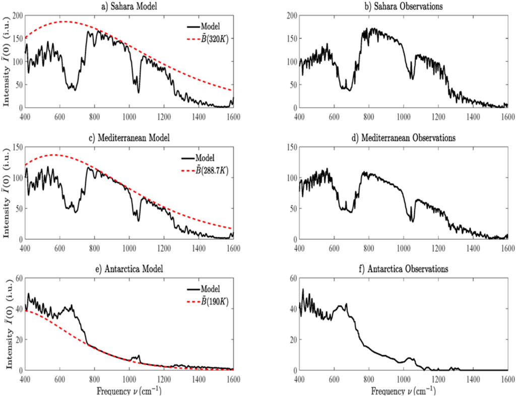
Figure 1. Reproduction of Figure 9 in van Wijngaarden and Happer (2025) (or Figure 10 in van Wijngaarden and Happer, 2023): Vertical intensities Ī(0) at the top of the atmosphere observed with a Michaelson interferometer in a satellite (Hanel and Conrath, 1970), and modeled with radiation transfer theory for the Sahara desert, Mediterranean and Antarctica. The “frequency” referred to in the horizontal axis should better read as “wavenumber”. The intensity unit in the vertical axis is 1 i. u. = 1 mW m⁻¹ cm sr⁻¹. The labels (a-f) are explained in each of the panels.

Some discrepancy appears in the Antarctica case, as the observed radiation is higher than that emitted by the Earth’s surface. The explanation given by van Wijngaarden and Happer (2023) and van Wijngaarden and Happer (2025) is this:

Radiative forcing is negative over wintertime Antarctica since the relatively warm greenhouse gases in the troposphere, mostly CO₂, O₃ and H₂O radiate more to space than the cold ice surface at a temperature of T = 190 K, could radiate through a transparent atmosphere.

We note though that the T = 190 K, as well as the entire atmospheric profile, are estimated, rather than observed. Hanel and Conrath (1970) mention that

no radiosonde data are available for comparison […] The profile can be anticipated intuitively from an examination of the spectrum […] The cold surface temperature results in the relatively low radiances found in the window region and between the water vapour lines.

Further examination of systematic ground temperature observations in the area shows that the assumed value of T = 190 K is unlikely. Specifically in the South Pole (station Amundsen-Scot; coordinates: 90°S, 0°E, prob: 2,770 m), the lowest daily temperature in April 1970 (the month of the experiment) did not fall below 204K. The Vostok station (coordinates: 78.45°S, 106.87°E, 3,420.0 m or prob: 3,468 m) is the location with the lowest temperatures among 41 GHCN-D stations in Antarctica, and its temperatures in April are, on average, 7 K lower than in Amundsen-Scot. Furthermore, the reconstructed vertical temperature profile given by Hanel and Conrath (1970) does not seem plausible as it has an abrupt increase of >30 K at the level of 700 hPa.

On the other hand, the ERA5 Reanalysis data suggest that there is a permanent state of temperature inversion (increasing temperature with increased altitude) between the atmospheric levels of 700 and 600 hPa (Figure 2), albeit not that big. This explains the discrepancy seen in Figure 1. The presence of the temperature inversion over the Antarctic Plateau has been studied by Sejas et al. (2018), who found that, along with the scarcity of free tropospheric water vapor, it causes a negative greenhouse effect. In addition, Lindzen (2012) stated that in the case of temperature inversion, RAGs actually cool, rather than warm, the atmosphere. (See additional explanation in Section 3.4 below.).

Figure 2

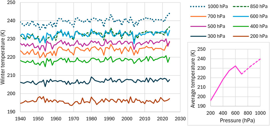
Figure 2. Evolution of mean monthly air temperature at the South Pole for the winter month that it is minimized at the indicated levels of the atmosphere. The inset on the right shows the average temperature vs. atmospheric pressure highlighting the inversion at pressure levels between 700 and 600 hPa. The pressure levels higher than 700 hPa (curves plotted as dashed lines) are not real as the altitudes are about 3,000 m, corresponding to about 700 hPa. Data from ERA5 Reanalysis retrieved through NOAA’s WRIT.

3.2 What would be the atmospheric temperature profile in equilibrium?

In their recent work, van Wijngaarden and Happer (2023) stated: “In the absence of greenhouse gases, the isothermal atmosphere will not change with time, since there is no thermal gradient to drive heat flow”. They also asserted that “without greenhouse gases, a thermally isolated adiabatic atmosphere would slowly evolve to an isothermal atmosphere because of conductive heat flow from the warmer lower atmosphere to the colder upper atmosphere”. Here we examine these statements with a slightly different formulation as seen in the question in the heading of this subsection.

It is well known that a gas in equilibrium tends to become isothermal, but here we examine the question also including gravity in the analysis. In fact, this problem is very old and is known as the Loschmidt paradox after Loschmidt (1876) who asserted that gravity could counteract the temperature uniformity implied by the second law as the kinetic energy of the molecules of a gas should be lower at higher elevation in compensation for the higher potential energy. The paradox puzzled many for years, yet both James Clerk Maxwell and Ludwig Boltzmann reacted negatively, supporting the isothermal hypothesis, as detailed in a recent analysis by Darrigol (2021).

Nonetheless, we deemed it useful to perform our own investigation in reply to this question independently of past arguments and using two methods. First, we maximize the entropy of a single molecule which is in motion in a vertical column under gravity. The single-molecule method has been successfully used before to derive the Clausius-Clapeyron equation (Koutsoyiannis, 2014). The development and application of the method to a spherical monoatomic and to a diatomic molecule are presented in Supplementary Appendices SB, SC, respectively. In brief, the thermal (internal) energy per molecule turns out to be the same for all altitudes, equal to ${\epsilon }_{\theta }=\beta \epsilon /\left(\beta +2\right)$, where $\beta$ is the number of degrees of freedom of a molecule and ε is its total energy. This results in $3\epsilon /5$ for monoatomic molecules and $5\epsilon /7$ for diatomic molecules. The remaining energy ${\epsilon }_g=2\epsilon /\left(\beta +2\right)$ is the average dynamic energy due to gravity. The temperature is also constant, independent of the altitude, equal to

$T=\frac{2{\epsilon }_{\theta }}{\beta k}=\frac{2\epsilon }{\left(\beta +2\right)k}(1)$

where k is the Boltzmann constant. In other words, entropy maximization results in an isothermal atmosphere.

The same result emerges when we approach the problem with our second method, without invoking the principle of maximum entropy—by instead simulating the motion of molecules, modeled as perfectly elastic hard spheres, using only Newton’s laws. Once again, the temperature is found to remain constant with altitude, as shown in Figure 3 and discussed in detail in Supplementary Appendix SD. In other words, none of the approaches predicts a decrease in temperature with altitude, which is the observed behavior as will be explained in Section 3.3.

Figure 3

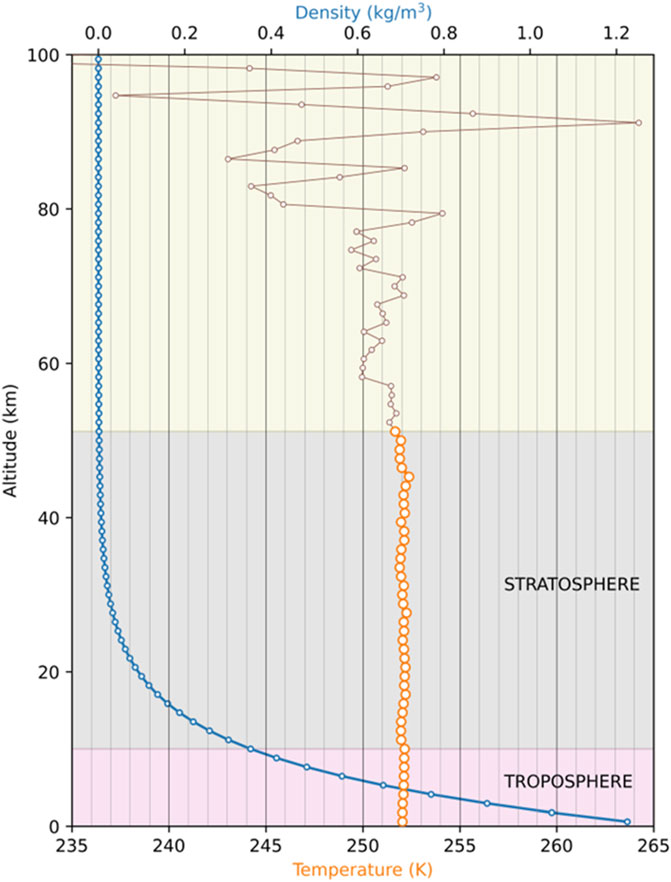
Figure 3. Reconstruction of the atmosphere’s density and temperature profile, based on the molecular dynamics simulation results. Simulation consisted of 100,000 gas molecules, doing 1.2 billion collisions within a periodic box with reflective bottom boundary. The fluctuations at high altitudes are deemed as statistical effects due to small samples.

3.3 What is the empirically observed temperature profile, and does it differ from the equilibrium profile?

It is common knowledge that Earth’s atmosphere is not isothermal. The temperature decreases with altitude in the troposphere, then it remains constant in the lowest layer of the stratosphere and continues to change at even higher altitudes. The typical atmospheric temperature profile is represented by the standard atmosphere adopted by the International Civil Aviation Organization (ICAO, 1993). According to the U.S. Standard Atmosphere (1976), the standard atmosphere is “A hypothetical vertical distribution of atmospheric temperature, pressure and density which, by international agreement, is roughly representative of year-round, midlatitude conditions.” It is based on large inventories of observational data and is widely used for meteorological and engineering applications. The vertical profile of temperature vs. altitude and atmospheric pressure is shown in Figure 4, with the temperature being 15°C or 288.15 K at the surface, linearly decreasing in the troposphere with the (minus) gradient $\mathrm{\Gamma }≔-\mathrm{d}T/\mathrm{d}z$ being 6.5 K/km up to the altitude of 11 km, and taking a constant value of 216.65 K above this up to 20 km.

Figure 4

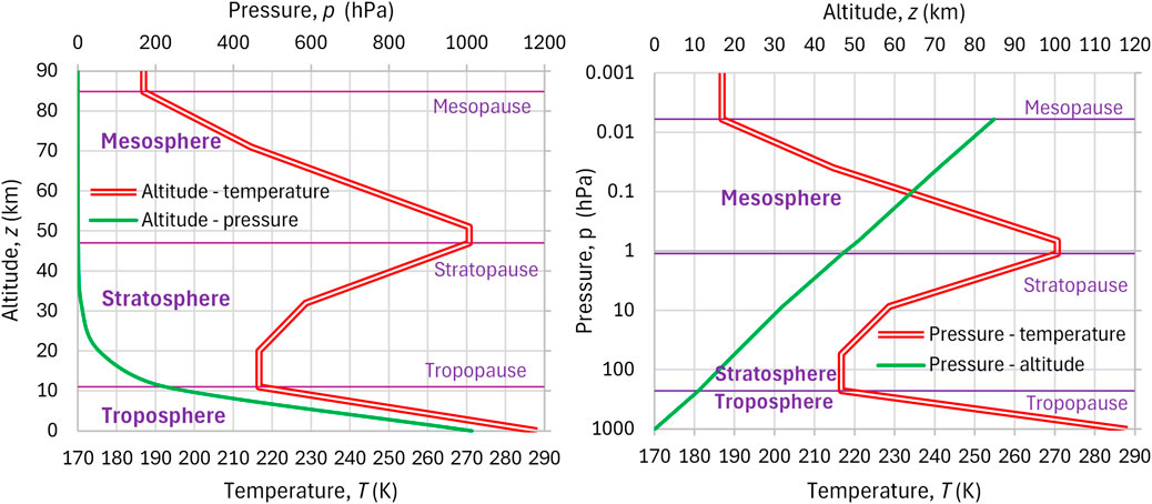
Figure 4. Vertical profiles of the ICAO (1993) standard atmosphere: (left) temperature and pressure as functions of altitude; (right) temperature and altitude as functions of pressure.

Clearly, the standard atmosphere is far from isothermal. Here we extensively use the standard atmosphere as satisfactorily representing reality, even though newer data and research (Wiencke, 2021) support slightly lower values of Γ, particularly at high latitudes. This will be verified below (Section 3.7). It is interesting to note that the average temperature in the standard atmosphere, calculated (by numerical integration) from the coordinates of Figure 4, is

$\overline{T}=\frac{{\displaystyle {\int }_0^{\infty }}T\left(z\right)\rho \left(z\right)\mathrm{d}z}{{\displaystyle {\int }_0^{\infty }}\rho \left(z\right)\mathrm{d}z}=250\mathrm{K}\left(=-23°\mathrm{C}\right)(2)$

where, by the ideal gas law, the air density $\rho$ is proportional to $p/T$, with $p$ denoting air pressure.

Figure 5 shows that temperature gradients appear in other planets and satellites in our solar system, and even in extrasolar planets (for additional rocky exoplanets see also Malik et al., 2019). In other words, isothermal atmospheres never seem to actually exist in planets.

Figure 5

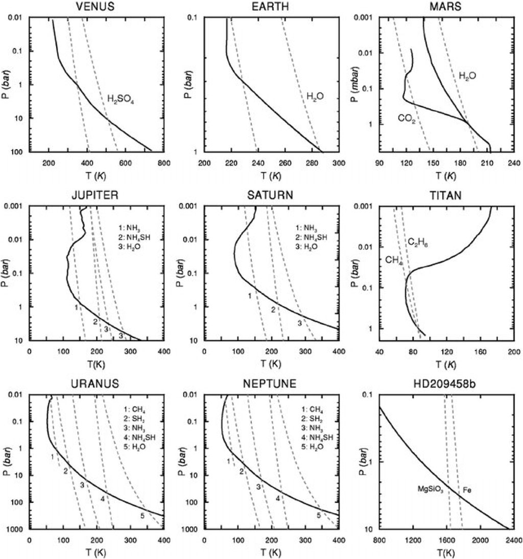
Figure 5. Vertical temperature profiles in the atmospheres of the indicated planets, the satellite Titan, and the extrasolar planet HD209458b (continuous lines), reproduced from Sánchez-Lavega et al. (2004), (Figure 3) with the permission of AIP Publishing. Saturation vapor pressure curves for the indicated condensates (substances forming clouds) for each planet are also plotted (dashed lines), details of which are given in the original publication.

Another important case, additional to the isothermal, is the isentropic atmosphere, where the per-molecule entropy is constant, independent of altitude. Following van Wijngaarden and Happer (2023) here we use the adjectives adiabatic and isentropic interchangeably, even though under some conditions, adiabatic processes can differ from isentropic processes. It is well known that in the absence of water vapor (dry conditions) the atmosphere has a constant temperature gradient equal to

${\mathrm{\Gamma }}_{\mathrm{d}}=\frac{g}{c_{p\mathrm{d}}}=9.8\mathrm{K}/\text{km}(3)$

where $g=9.81$ m/s is the gravity acceleration (typical value for the troposphere) and $c_{p\mathrm{d}}=1004$ J kg^–1 K⁻¹ is the specific heat capacity of the dry air for constant pressure. This is depicted in Figure 6 for the troposphere and lower stratosphere.

Figure 6

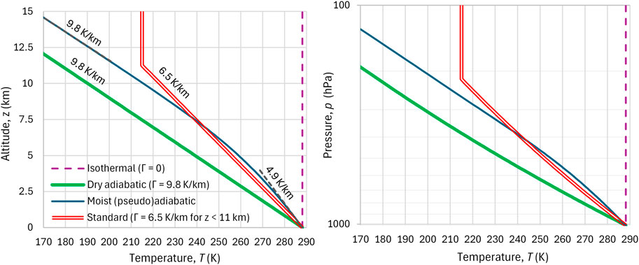
Figure 6. Comparison of different models of temperature profiles of Earth’s troposphere, in terms of (left) altitude and (right) pressure (in logarithmic axis).

Another limiting case is the moist (pseudo-)isotropic profile, also shown in Figure 6. To calculate it we have used the following equation (Beers, 1945, p. 359; Koutsoyiannis, 2000) which gives a satisfactory approximation for both the isentropic change of saturated air (in which the liquid water remains in the space considered) and saturated pseudo-adiabatic change (in which the liquid water precipitates immediately):

$c_{p\mathrm{d}}\ln T-R_{\mathrm{d}}\ln \left(p-e\left(T\right)\right)+\frac{\lambda r\left(T\right)}{T}=\text{const}(4)$

In this, $R_{\mathrm{d}}=287$ J kg^–1 K⁻¹ is the gas constant of dry air, $\lambda =\left(3.139\times {10}^6-2336T/\mathrm{K}\right)$ J kg^–1 is the latent heat of vaporization, and $e\left(T\right)$ and $r\left(T\right)$ are the saturation water vapor pressure and mixing ratio, respectively, for temperature T. By taking derivatives in Equation 4, setting $e\left(T\right)=r\left(T\right)=0$, and performing algebraic manipulations we readily find as a special case Equation 3 for dry conditions.

The saturation water vapor pressure $e\left(T\right)$ is given by the Clausius-Clapeyron equation, as reformulated for water vapor by Koutsoyiannis (2012):

$e\left(T\right)=e_0\exp \left(24.921\left(1-\frac{T_0}{T}\right)\right){\left(\frac{T_0}{T}\right)}^{5.06},T_0=273.16\mathrm{K},e_0=6.11657\text{\hspace{0.17em}hPa}(5)$

with T₀ and e₀ representing the coordinates of the triple point of water. The mixing ratio is

$r\left(T\right)=\frac{\epsilon e\left(T\right)}{p-e\left(T\right)}(6)$

where ε = 0.622 is the ratio of molar masses of water vapor and dry air.

It is seen in Figure 6 that the moist adiabatic atmosphere does not have a constant temperature gradient. Rather the gradient is low (4.9 K/km) at the surface and becomes equal to the dry adiabatic rate (9.8 K/km) at high altitudes. This is a consequence of the fact that at low temperatures the saturation vapor pressure is close to zero and, as already explained, Equation 4 switches to Equation 3. The standard atmosphere has a profile close, but not identical, to that of the moist adiabatic one. Its slope is constant (6.5 K/km) for the entire troposphere. The differences become large at high altitudes near the tropopause and above.

It is useful to compare these profiles with observational data. To this aim, we enroll in the ERA5 reanalysis over the period 1940 – 2024 and find the global average temperature over this period at the available pressure levels, as well as the global average geopotential heights for these pressure levels. The results, areally averaged over the torrid and the north frigid zones, are shown in Figure 7. To adapt the standard profile to the conditions of Figure 7 we take the following steps: (a) we replace the standard ground temperature of 288.15 K with the average temperature of the zone at 1,000 hPa, (b) we apply the standard gradient Γ = 6.5 K/km up to the altitude where the temperature takes the standard stratospheric value of 216.65 K, and (c) we keep a constant value of 216.65 K above this altitude up to 20 km.

Figure 7

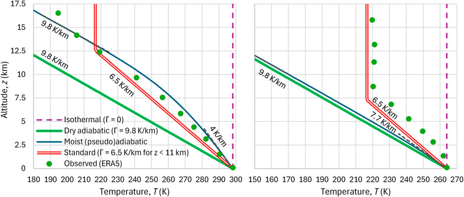
Figure 7. Comparison of temperature profile models of Earth’s troposphere with the mean annual observed temperature profile as given by ERA5 reanalysis, temporally averaged over the period 1940 – 2024 and areally averaged over (left) the torrid zone and (right) the north frigid zone.

We observe that in the tropics the actual average temperature profile is located between those of the moist adiabatic and the standard atmosphere, but above 12.5 km it is closer to the former than the latter. However, in the polar area, observations are totally irrelevant to the moist adiabatic profile. Notice that the moist adiabatic conditions would suggest greater gradients in colder conditions (right panel) than in hotter (left panel) because of the Clausius-Clapeyron equation which results in lower WV quantities for lower temperatures (compare the gradients at the surface level, 4.0 and 7.7 K/km in the two panels). The reality is the exact opposite as seen in Figure 7 (see also Figures 12, 13 below). This means that the moist adiabatic process, despite often being invoked in the literature to explain atmospheric conditions, is not sufficient a tool to describe and explain what happens in reality. All these support the conclusion that the standard atmosphere, despite its empirical basis and its low explanatory power, is more representative for the entire range of conditions on Earth, while the moist adiabatic profile is representative only for the tropics. The dry adiabatic profile is always very different from average conditions. For this reason, the analyses that follow are based on the standard atmosphere.

3.4 Is the ARE responsible for the observed temperature profile in the atmosphere?

To address the question in the heading, we apply the established greenhouse theory, without considering doubts that have been cast on the validity of the theory or alternative hypotheses (e.g., Nikolov and Zeller, 2017; Miskolczi, 2023). Rather, we enroll the RRTM software, which calculates at each atmospheric level z the SW and LW radiation going up and down, namely, the four quantities $R_{\mathrm{S}{\mathrm{W}}_{\text{up}}},R_{\mathrm{S}{\mathrm{W}}_{\text{down}}},R_{\mathrm{L}{\mathrm{W}}_{\text{up}}},R_{\mathrm{L}{\mathrm{W}}_{\text{down}}}$. The algebraic sum of the four quantities for $z$ equal to the ground level is the net radiation balance at the surface, which is used in evaporation calculations. While, due to its “rapid” characteristic this software is not the most accurate, we deem it satisfactory for the exploratory character of this research. Taking the differences at two adjacent levels $z_1,z_2$ we calculate the quantities $\Delta R_{\mathrm{S}{\mathrm{W}}_{\text{up}}},\Delta R_{\mathrm{S}{\mathrm{W}}_{\text{down}}},\Delta R_{\mathrm{L}{\mathrm{W}}_{\text{up}}},\Delta R_{\mathrm{L}{\mathrm{W}}_{\text{down}}}$, the total radiative energy imbalance $\Delta R_{\text{tot}}$, and finally the radiative energy imbalance slope, REIS, based on the following equations.

$\Delta R_{\text{tot}}≔\Delta R_{\mathrm{S}{\mathrm{W}}_{\text{up}}}+\Delta R_{\mathrm{S}{\mathrm{W}}_{\text{down}}}+\Delta R_{\mathrm{L}{\mathrm{W}}_{\text{up}}}+\Delta R_{\mathrm{L}{\mathrm{W}}_{\text{down}}},\text{REIS}≔\frac{\Delta R_{\text{tot}}}{\Delta z}(7)$

By convention, $R$ quantities directed up are taken as positive and those directed down as negative. If REIS turns out to be positive at a certain layer, between the levels $z_1,z_2$, this means that the layer receives energy of another type, such as sensible or latent thermal energy. This should be equal to REIS, so that the total energy balance be reinstated.

Figure 8 depicts examples of these quantities between the elevations z = 0 and z = 426 m (the fourth altitude given as output by RRTM) and for conditions specified in the figure caption, which include both RAGs and clouds. Two cases are examined, an isothermal atmosphere (Γ = 0) and the standard atmosphere (Γ = 6.5 K/km). In the former case, REIS is almost zero, which means that no forcing appears to drive the atmospheric state away of the equilibrium. Therefore, the atmosphere would remain at the equilibrium (isothermal) state, despite the presence of RAGs and clouds.

Figure 8

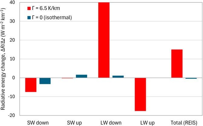
Figure 8. Radiative energy change (SW and LW) between the elevations z = 0 and z = 426 m and for the indicated cases with default values of RRTM plus clouds, both low and high, each with a fraction of 0.5. For an isothermal atmosphere (Γ = 0) the REIS is almost zero, while for the standard atmosphere gradient (Γ = 6.5 K/km) there is a positive REIS, implying the presence of other energy forms to balance energy.

In contrast, for the standard atmosphere gradient a positive REIS appears, which means that the total energy balance needs to be reinstated by other energy forms. These forms are indeed present and are the sensible heat due to warm air parcels moving from the Earth’s surface up, and the latent heat due to evaporation, again moving from the surface up.

A more complete picture is provided in Figure 9, where REIS is calculated and plotted for the entire range of altitudes modeled by RRTM, for four different cases of ARE (RAG with clouds, RAG without clouds, no NC-RAG with clouds, no NC-RAG without clouds) and for two cases of temperature gradient, Γ = 6.5 K/km (standard atmosphere; upper row of panels) and Γ = 0 (isothermal atmosphere, lower row of panels). What was discussed with respect to Figure 8 is confirmed in Figure 9 for all cases examined and for all altitudes in the troposphere. The isothermal case yields almost zero REIS in the entire troposphere (z < 11 km) in all cases, which means that the presence of RAGs, whether NC or WV, is not enough for the observed gradient to emerge, nor for the ARE to appear.

Figure 9

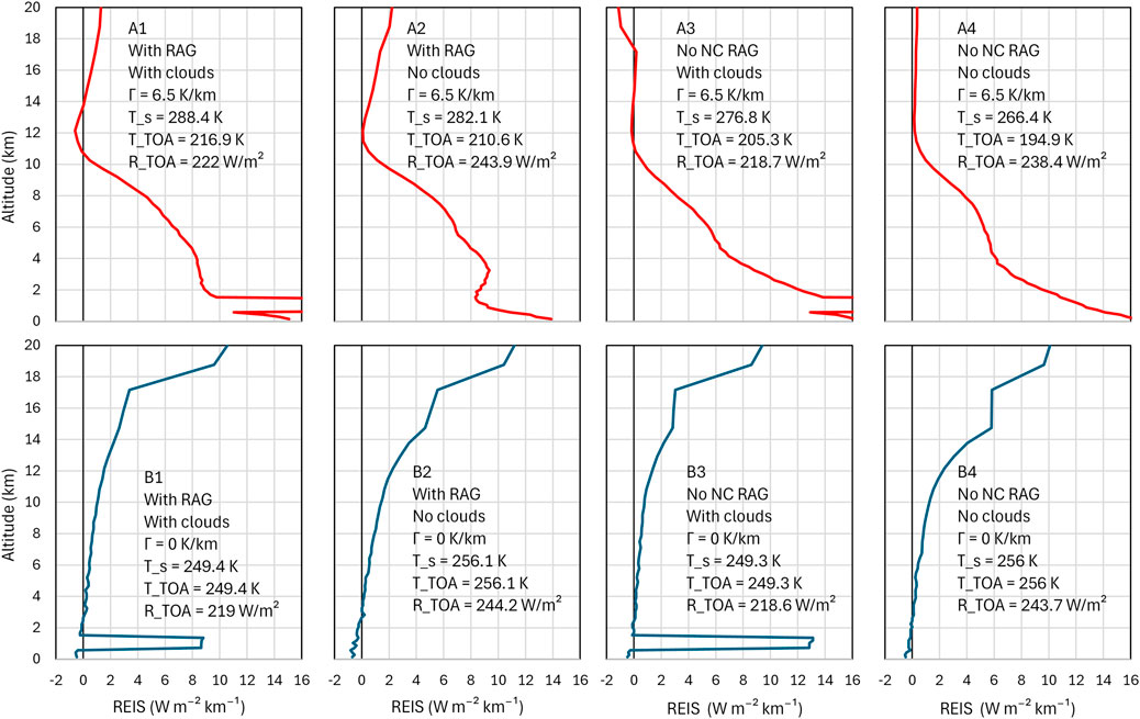
Figure 9. Total (SW and LW) radiative energy imbalance as a function of altitude for the indicated cases. In the upper row the gradient is Γ = 6.5 K/km, as in the standard atmosphere, while in the lower row there is no gradient (isothermal atmosphere, Γ = 0). The temperature at the surface (T_s) and the top of atmosphere (T_TOA) are determined by the RRTM so as to equilibrate the incoming net SW (incoming minus outgoing) and the outgoing LW radiation at the top of atmosphere (R_TOA). The default values of RRTM parameters are used wherever it is not noted otherwise. In cases A1, A3, B1 and B3 the clouds referred to are both low and high, each with a fraction of 0.5. The spikes appearing at altitudes around 1 km are due to low clouds. Although in an isothermal atmosphere, clouds would not be formed, for comparison the imaginary cases B1 and B3 assume the existence of clouds, similar to cases A1 and A3.

The last observation may sound counterintuitive to many who regard the presence of RAGs as a sufficient reason for the temperature gradient. However, our finding is consistent with experimental evidence reported by Harde and Schnell (2022), who stated:

the greenhouse effect is mainly the result of a temperature difference over the propagation path of the radiation and thus the lapse rate in the atmosphere.

It further agrees with the following two statements by Lindzen (2012) and Lindzen (2018), respectively):

It should be emphasized that if dynamical mixing were to have led to an isothermal atmosphere, then there would be no warming due to added greenhouse gases. In the counterfactual case that mixing were to have lead to increasing temperature with altitude, then added greenhouse gases would actually cool the atmosphere. In brief, greenhouse warming depends crucially on the existence and properties of dynamic mixing within the troposphere, and not simply on the radiative picture.

It is an interesting curiosity that had convection produced a uniform temperature, there wouldn’t be a greenhouse effect.

On the other hand, with the standard atmosphere gradient (Γ = 6.5 K/km) there is a positive REIS in the entire troposphere, which leaves room for sensible and latent heat to act, reinstating the total energy balance and stabilizing the temperature gradient.

3.5 What factors can explain the observed temperature profile?

Given the analysis of the previous subsection, it becomes clear that it is not the ARE that creates and maintains the temperature gradient. Rather the mechanisms responsible for the temperature gradient are:

• the warming of the soil and liquid water by the sunshine during the day and their cooling during the night;

• the water evaporation and transpiration at the surface level and condensation aloft;

• the convection, and the implied vertical transfer of sensible and latent heat;

• the winds caused by spatial temperature differences and influenced by Coriolis forces.

These are not static forcings, but processes, i.e., perpetual changes in the climatic system. The processes occur on different time scales, some of which are too small to drive the atmosphere to the equilibrium (isothermal) state. It is noted that the processes occur at a macroscopic level, with the motion of masses of air, typically referred to as parcels. And as noted by van Wijngaarden and Happer (2023), because of the very small thermal conductivity of air, it takes a very long time for appreciable heat to flow into or out of a parcel of reasonable size.

The driving mechanisms of these processes are the following:

1. Clouds form and disappear, strongly affecting the SW and LW radiation processes.

2. The Earth’s surface is not homogeneous in terms of radiation absorption and reflection (varying albedo). The massive presence of water in liquid and solid phases with different albedo values, both on the Earth’s surface (hydrosphere, cryosphere) and in the atmosphere (clouds) is responsible for spatial and temporal variations in the albedo, as well as in the thermodynamic properties of different parts of the Earth.

3. Earth is round (not flat) and the sunrays come with different slopes at different places.

4. Earth rotates around its axis on a daily basis.

5. Earth rotates around the Sun on an annual basis.

6. Earth’s orbit around the Sun is elliptical, resulting in changes in the distance between the two bodies.

7. The climatic system is complex and is subject to irregular changes.

A rough quantification of changes produced by these mechanisms is shown in Table 2, where it is seen that some of them are of the order of 100%, reaching the absolute maximum of 200% on a daily scale. This quantification is just indicative and is unable to quantitatively predict the observed temperature profiles as seen in Figure 7. It is also unable to produce the standard temperature gradient of 6.5 K/km, which here we regard as an empirical model with satisfactory accuracy in representing the average conditions over the entire globe. It incorporates all mechanisms discussed here, but it can hardly be inferred from them by deduction. Sometimes the literature connects it to the moist adiabatic profile but the data above (particularly the right panel in Figure 7) do not support this idea.

Table 2

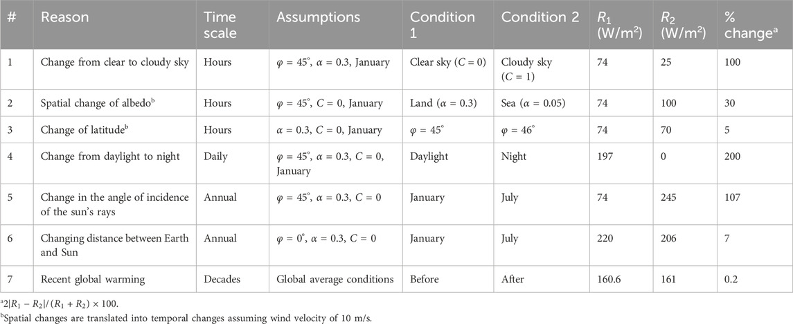
Table 2. Typical changes that cause departure from the isothermal atmosphere and their quantified effect on SW radiation processes. R₁ and R₂ denote the downwelling solar radiation at the surface level for the specified conditions 1 and 2, respectively; φ, α and C denote the latitude, albedo and cloudiness, respectively. The calculations are based on Koutsoyiannis (2000) and van Wijngaarden and Happer (2023).

3.6 What is the relative importance of ARE and temperature gradient in climate dynamics?

The information provided in the different panels of Figure 9 includes the surface temperature at each of the cases examined (A1-A4, B1-B4). A summary of the results is given in Figure 10, along with some additional hypothetical cases. The first imaginary-world case is a planet shaped as a disk perpendicular to the Sun’s rays, without an atmosphere and receiving the average radiative energy that the Earth does. In this case, the so-called effective temperature is easy to calculate from the Stefan-Boltzmann law, i.e.,

$T_0={\left(\frac{I}{4}\frac{1-\alpha }{\epsilon \sigma }\right)}^{\frac{1}{4}}(8)$

where I = 1360 W/m² is the solar irradiance with I/4 = 340 W/m² representing the average solar energy received by (the spherical) Earth’s surface, while σ = 5.67 × 10⁻⁸ W m⁻² K⁻⁴ is the Stefan–Boltzmann constant, ε is the emissivity of the radiating body and α is its albedo. Taking ε = 1 and using the Earth’s current albedo $\alpha =0.3$, so that $\left(I/4\right)\left(1-\alpha \right)=238$ W/m², the result is $T_0=$ 254.5 K.

Figure 10

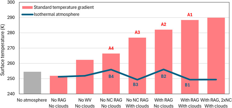
Figure 10. Surface temperature for the cases shown in Figure 9 (A1-A4, B1-B4), in comparison with four additional hypothetical cases: the three cases on the left are for no atmosphere, no RAGs at all and no WV (and hence no clouds); the rightmost case is similar to A1/B1 but with doubled NC-RAGs, resulting in zero change for the isothermal atmosphere (compared to B1) and 1.5 K increase for an atmosphere with standard gradient (compared to A1).

About the same (T = 252 K) would be the temperature in the imaginary-world case where there is an atmosphere but no ARE (no RAG and no clouds; second bar in Figure 10) or even with NC-RAGs, but without WV and clouds and without a temperature gradient. If the gradient of 6.5 K/km is present (third bar in Figure 10) the temperature increases to 262 K. Therefore, the effect of the NC-RAGs is zero for an isothermal atmosphere and 10 K for an atmosphere with temperature gradient of 6.5 K/km. By no means is it close to about 30 K as typically implied in the literature.

In general, in an isothermal atmosphere, the effect of RAGs, including NC-RAGs, WV and clouds, is practically zero, as shown by the continuous (blue) line in Figure 10, which fluctuates only slightly, from 249 to 256 K. In contrast, if there is a gradient of 6.5 K/km, the temperature increases up to ∼288 K in the realistic case A1, in which the atmosphere contains all RAGs and clouds.

Hence, it is the temperature gradient that makes the surface-level temperature increase from about 252 K (which is close to the average $\overline{T}=$ 250 K of Equation 2) to about 288 K (i.e., by 36 K). This increase is usually attributed to the “greenhouse effect”, but it is mainly the result of the temperature gradient, whose origin is not the ARE but the processes described in section 3.5. This is another reason why it is necessary to stop using the term “greenhouse effect” when talking about the climatic system.

We stress that, among the various cases shown in Figure 10, only cases A1 and A2 are realistic, while all the others are hypothetical. A final hypothetical case shown at the rightmost end of the figure is where the NC-RAGs are doubled. This results in a temperature increase of zero in comparison to case B1 or 1.5 K in comparison to case A1.

While the temperature gradient is the determinant factor that maintains the Earth’s temperature much higher than the effective temperature of 254.5 K, with the mechanisms causing this gradient being also causes of maintaining warm conditions, the RAGs also play a significant role as can be inferred from Figure 10. An atmosphere free of RAGs (both WV and NC) and clouds would keep the temperature close to the average, i.e. 252 K (second bar in Figure 10). However, this case is equally imaginary as that of no atmosphere (first bar in Figure 10) and does not represent planet Earth. For Earth is massively (71%) covered by water, which evaporates, thus giving rise to WV and clouds in the atmosphere. Even without NC-RAGs but with WV and clouds, the surface temperature would be 277 K (case A3)—a substantial increase with respect to the effective temperature.

While Figure 10 provides information on the importance of different agents of Earth’s warming, it should be stressed that the figure compares the realistic cases (A1, A2) with several imaginary-world cases (all others). Hence, it cannot be a basis for understanding the importance of each factor in real-world conditions. The scientific approach for the latter task is to determine the partial derivatives of a suitable multivariate function representing the ARE, such as the downwelling or outgoing LW radiation, at the point of the current conditions and compare them. Such an analysis has been done in Koutsoyiannis (2024b) with the following resulting percent contributions: (a) for downwelling LW radiation, WV and clouds 95%, CO₂ 4%, all other 1%; (b) for outgoing LW radiation, WV and clouds 87%, CO₂ 5%, all other 8% (primarily due to the influence of the stratospheric ozone).

Water vapor, besides being the determinant RAG and the cause of clouds, also has overwhelmingly more impact than CO₂ because its quantity in the atmosphere varies substantially over time and space. This makes WV an agent of perpetual change on all time scales. Relevant changes, mostly on hourly to annual time scales, have already been described in Section 3.5. However, changes also occur at decadal, centennial scales and beyond. These long-term changes are inherent in all geophysical processes, including hydroclimatic ones, and are described in stochastic terms by the so-called Hurst-Kolmogorov dynamics (Koutsoyiannis, 2013; Koutsoyiannis, 2021; Koutsoyiannis, 2024a; O’Connell et al., 2016; Dimitriadis et al., 2021).

As far as long-term changes are concerned, the CERES satellite data show a decline in the albedo of about 0.004 for the entire observation period (post 2000), which translates to 1.4 W/m² (higher than the average imbalance of 0.4 W/m² shown in case 7 of Table 2). This is consistent with an observed decline in cloud area fraction (Koutsoyiannis et al., 2023; Appendix A.2, Koutsoyiannis and Vournas, 2024; Appendix B; see also Goode et al., 2021; Nikolov and Zeller, 2024). Interestingly, a recent study by Goessling et al. (2025) identifies a record-low planetary albedo in 2023, apparently caused largely by a reduced low-cloud cover in the northern mid-latitudes and tropics, in continuation of a multi-annual trend, all of which contributing to the recent global temperature surge.

Coming back to the results shown in Figure 10, a relevant issue to stress is that the analysis made is unidimensional. Is that representative for the average condition of Earth, which is spherical? A negative reply has been suggested by Nikolov and Zeller (2017), who showed that the mean physical temperature of a spherical body is always lower than its effective radiating temperature computed from the globally integrated absorbed solar flux. This happens because of Hölder’s inequality between integrals and the fact that Stefan-Boltzmann law is a power law with an exponent 4.

This suggestion indeed makes sense for the condition of a planet without an atmosphere (first bar in Figure 10), where an integration over the Earth’s sphere would result in a lower value than shown in the figure. However, if we consider the realistic conditions of Earth, in particular cases A1 and A2 of Figure 10, rather than the imaginary-world conditions, the cautionary note by Nikolov and Zeller does not apply. For the relationship between outgoing radiation and temperature is no longer a power law but a virtually linear relationship, as shown in Figure 11, constructed from CERES radiation data and ERA5 Reanalysis near-surface temperature data. Additional information on this linear relationship is provided by Koll and Cronin (2018), Figure 1 and Koutsoyiannis (2024b), Figure 6, which in essence confirm early observations and analyses by Budyko (1969). Hence, the quantities depicted in Figure 10 are representative of average conditions for the (spherical) Earth, at least for the realistic cases A1 and A2, albeit not for the imaginary case of an atmosphere-free Earth.

Figure 11

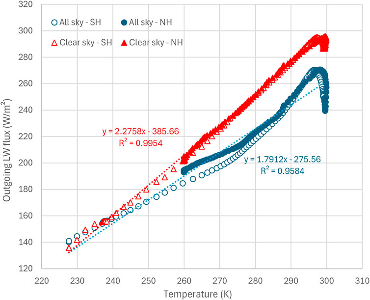
Figure 11. Outgoing LW radiation vs. ground temperature. Each point refers to the zonal average of LW radiation (for clear sky and all sky) averaged from 2000 to 2022 as given by the CERES data and the zonal average of ground temperature as given by ERA5 Reanalysis; the resolution is 1° (180 points in total). Temperature data from ERA5 Reanalysis retrieved from the CLIMEXP platform; radiation data retrieved from https://ceres-tool.larc.nasa.gov/ordtool/jsp/SSF1degEd41Selection.jsp.

3.7 What are the recent changes in the atmospheric temperature gradient?

Once we have recognized that the temperature gradient is a result of macroscopic changes on Earth (Section 3.5) and that it is a critical factor determining the climate (Section 3.6), it is useful to monitor and analyze its changes, which are certainly much more influential than the famed changes in CO₂ concentration. To this end, Figure 12 (upper) shows the variation of the atmospheric temperature averaged over the five geographical zones at two pressure levels, 1,000 and 200 hPa, as given by the ERA5 reanalysis.

Figure 12

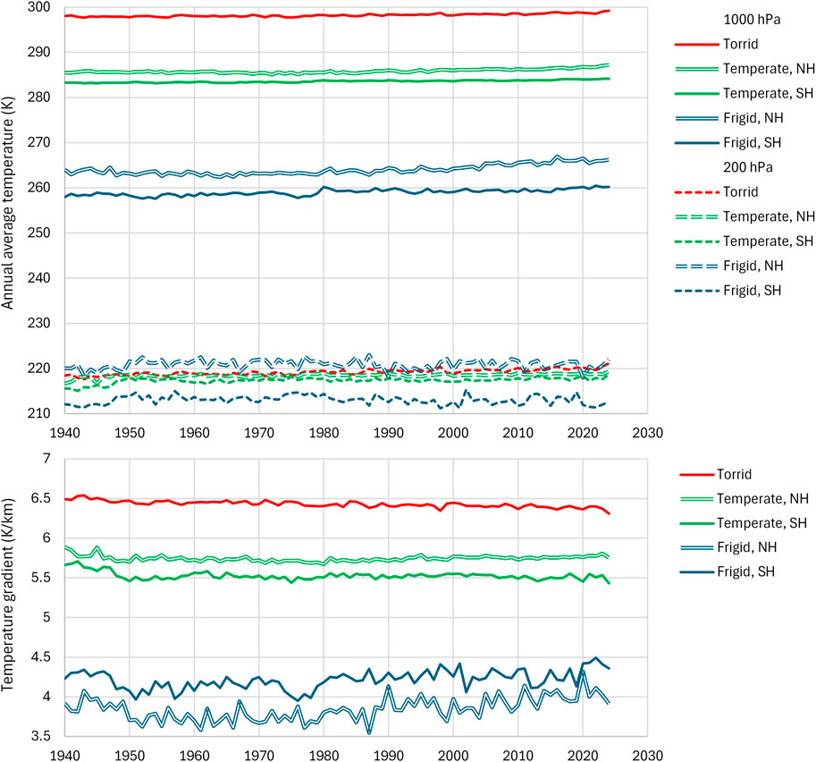
Figure 12. (upper) Evolution of mean annual air temperature averaged over the five geographical zones at the levels of 1,000 and 200 hPa. (lower) Evolution of the (minus) vertical temperature gradient per geographical zone, calculated from differences of temperatures and geopotential heights between these two levels. Data from ERA5 Reanalysis retrieved through NOAA’s WRIT.

By using the geopotential height at these pressure levels, also available in the ERA5 dataset, we determined and plotted in Figure 12 (lower) the evolution of the vertical temperature gradient per geographical zone, calculated as the (minus) ratio of differences of temperature and geopotential heights between these two levels.

It is clear from Figure 12 that, as we move from the equator to the poles and the surface temperatures decrease, so do the temperature gradients. This is fully compatible with the analyses of Sections 3.4–3.6, according to which higher gradients lead to higher surface temperatures (see also Figure 13, left).

Figure 13

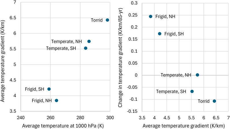
Figure 13. (left) Average temperature gradient per geographical zone (calculated as indicated in the caption of Figure 12) vs. average temperature. (right) Change in temperature gradient per geographical zone over the 85-year period of ERA5 data availability (calculated from the slope of linear trends fitted to the curves of Figure 12, lower).

Surface temperatures present increasing trends over time in all zones. In contrast, the temperatures at the level of 200 hPa do not show geographical or temporal changes. It is interesting to examine the temporal trends of temperature gradients, visualized in Figure 12 (lower) and summarized in Figure 13 (right). At the torrid zone we observe a falling trend, which can be viewed as negative feedback to the increasing surface temperatures. In contrast, at the frigid zones the trends are increasing, and hence we would expect greater warming. In the temperate zones no notable trends appear.

Indeed, the zonal distribution of the climatic surface temperature differences between the latest and oldest 30-year periods (for which ERA5 Reanalysis data are available in the CLIMEXP platform), seen in Figure 14, confirm these observations. The figure plots show that for the greatest part of Earth, between latitudes 50°S and 50°N there has been a warming trend of about 1.4 K/century, slightly increasing as we move north, as the percentage of land increases. Between 50°N and the Arctic Circle there is a further warming trend, while between 50°S and the Antarctic Circle the trend becomes cooling. The greatest increases of surface temperature are observed in the frigid zones, where we have increasing temperature gradient trends.

Figure 14

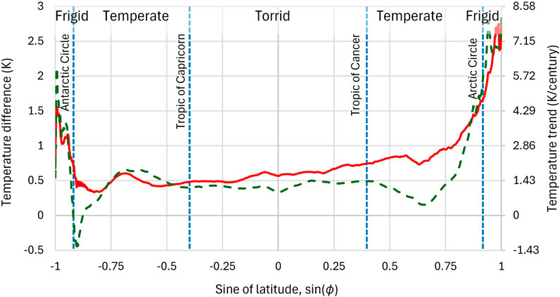
Figure 14. Difference of average surface temperatures, as a function of the sine of latitude, of two 30-year climatic periods, namely, of the most recent 1995 – 2024 minus the 1950 – 1979. Continuous line represents the average over the globe, while dashed line represents the average over the area between longitudes 155°E and 130°W, mostly covered by sea (Pacific, Arctic and Southern Oceans). The sine of latitude was chosen as the horizontal axis so that increments be proportional to the respective areas on Earth. Data from ERA5 reanalysis; data retrieval and processing from the CLIMEXP platform (processing steps: (a) subsetting for each of the two periods; (b) aggregation to annual (Jan-Dec) time resolution; (c) compute zonal mean; (d) compute mean, s.d. [standard deviation], or extremes).

All the above observations are consistent with the evidence from paleoclimatic studies, which suggests that the surface equator-to-pole temperature gradients were weaker during warm periods, while tropical temperatures changed very little (Budyko, 1977, p. 17; Huber et al., 2000, p. 289; Huber, 2008; Lee, 2014; Lindzen, 2020). They are also consistent with the recent study by Ma et al. (2025), which identified wind stilling (compatible with the decrease in the surface equator-to-pole temperature gradient), resulting in weaker evaporation in two-thirds of the ocean and a slight decreasing trend in global-averaged ocean evaporation during 2008–2017. In addition, as already mentioned, the falling multiyear trend in the planetary albedo, largely caused by a reduced low-cloud cover, has been a main driver of the recent global temperature.

4 Discussion and conclusions

The research presented here challenges the ideas that we live in a greenhouse and that science can be settled, and revisits the most fundamental topics related to climate. This is attempted in the simplest possible way and using the fewest premises, such as Newton’s laws, the principle of maximum entropy and the spectroscopic properties of gases. Additionally, the study proposes that commonly used vocabulary should be replaced by rigorous scientific terminology, the main examples being “greenhouse gas” and “greenhouse effect”, which could be replaced by “radiatively active gas” (RAG, comprising water vapor—WV—and non-condensing radiatively active gases—NC-RAGs) and “atmospheric radiative effect” (ARE), respectively.

The conclusions of the analyses presented here can be summarized as follows:

• There is an empirically verified ARE in the atmosphere, not only on Earth but also on the other planets. On Earth, ARE is dominated by WV and clouds, with CO₂ playing a very minor role—let alone human added CO₂ which represents only 4% of the total emissions to the atmosphere.

• Equilibrium thermodynamics clearly show (either using the principle of maximum entropy, or stochastic simulation of molecule collisions) that Earth’s atmosphere would be isothermal at the equilibrium, with or without RAGs. In an isothermal atmosphere the temperature would be slightly higher than 250 K, a value which represents the vertically average temperature of the standard atmosphere over the troposphere and stratosphere.

• The fact is that the atmosphere is not isothermal. Rather, the troposphere has a vertical temperature gradient of about 6.5 K/km, which is imprinted in the standard atmosphere. The gradient is resultant of macroscopic changes that drive the atmosphere out of equilibrium. While the moist adiabatic changes play a role in shaping this gradient, they cannot fully predict real atmospheric conditions.

• The mean surface temperature of 288 K, also imprinted in the standard atmosphere, is much higher than the equilibrium temperature. While RAGs (mostly WV and clouds) play a role in yielding this temperature, the critical factor is the vertical temperature gradient, without which the ARE alone would not be able to increase the equilibrium temperature.

• Given the importance of the atmospheric temperature gradient, which is described by large-scale atmospheric thermodynamics, rather than radiative physics, it is puzzling that the emphasis in climate research has been on the latter. This gradient is not a universal constant, but it varies with space and time. It is therefore useful to monitor and analyze its changes. The data show that since 1950 the gradient has weakened in the tropics and grown in the polar areas resulting in decrease of the surface equator-to-pole gradient, as expected in global warming conditions.

A final point worth stressing is that in complex systems, such as the climatic system, observational data are the only scientific test bed for making hypotheses and assessing their validity. Focusing on one of the factors affecting the climatic system, namely, the anthropogenic CO₂ emissions, and basing on models that emphasize this factor, may distort our perception of the big picture and be detrimental to science, whose objective is to pursue the truth.

Data availability statement

The datasets presented in this study can be found in online repositories, namely in the links given in section 2 and the references cited there.

Author contributions

DK: Data curation, Supervision, Conceptualization, Software, Investigation, Methodology, Writing – original draft, Writing – review and editing, Resources, Project administration, Validation, Formal Analysis. GT: Validation, Visualization, Writing – review and editing, Methodology, Formal Analysis, Investigation, Software.

Funding

The author(s) declare that no financial support was received for the research and/or publication of this article.

Acknowledgments

We are grateful to the colleagues and organizations who have put their huge data sets online along with the data processing and computational systems they have developed. These include the CERES data, the ERA5 Reanalysis, the CLIMEXP and WRIT data and software platforms, and the RRTM software system. We thank two reviewers for the positive assessment of the paper and their detailed and constructive comments. We also thank the Guest Editors and Chief Editors for the processing of the paper and their suggestions, and for approving the paper for publication. We acknowledge useful comments (including points of disagreement) on a preprint of the paper (doi: 10.13140/RG.2.2.14752.49923) which we received from Ned Nikolov, William Happer, Willis Eschenbach, Hermann Harde and Richard Cina. All the above helped us improve the final version of the paper.

In memoriam

Dedicated to the memory of Anna (Annouska) Patrikiou–Koutsoyiannis, who left this world while this research was conducted.

Conflict of interest

The authors declare that the research was conducted in the absence of any commercial or financial relationships that could be construed as a potential conflict of interest.

Generative AI statement

The author(s) declare that no Generative AI was used in the creation of this manuscript.

Publisher’s note

All claims expressed in this article are solely those of the authors and do not necessarily represent those of their affiliated organizations, or those of the publisher, the editors and the reviewers. Any product that may be evaluated in this article, or claim that may be made by its manufacturer, is not guaranteed or endorsed by the publisher.

Supplementary material

The Supplementary Material for this article can be found online at: https://www.frontiersin.org/articles/10.3389/fcpxs.2025.1617092/full#supplementary-material

References

Ångström, A. (1915). A study of the radiation of the atmosphere based upon observations of the nocturnal radiation during expeditions to Algeria and to California. Smithsonian miscellaneous collections, 65. Washington DC, USA: Smithsonian Institution Publication, 159. Available online at: https://repository.si.edu/handle/10088/23534.3

Google Scholar

M. C. Barth, and J. G. Titus (1984). Greenhouse effect and sea level rise: a challenge for this generation (New York: Van Nostrand Reinhold), 360. Available online at: https://archive.org/details/greenhouseeffect0000unse_e4l4/.

Google Scholar

Beers, N. R. (1945). “Meteorological thermodynamics and atmospheric statics,” in Sec. V in handbook of meteorology. Editors F. A. Berry, E. Bollay, and N. R. Beers (New York: McGraw-Hill).

Google Scholar

Bernard Jr, H. W. (1980). Greenhouse effect. Cambridge, Massachusetts, USA: Ballinger Publishing, 216. Available online at: https://archive.org/details/greenhouseeffect0000bern.

Google Scholar

B. Bolin, B. R. Döös, J. Jäger, and R. A. Warrick (1986). The greenhouse effect, climatic change and ecosystems (Chichester, New York, USA: Wiley), 541. Available online at: https://archive.org/details/greenhouseeffect00boli/.

Google Scholar

Budyko, M. I. (1969). The effect of solar radiation variations on the climate of the Earth. Tellus 21 (5), 611–619. doi:10.1111/j.2153-3490.1969.tb00466.x

CrossRef Full Text | Google Scholar

Budyko, M. I. (1977). Climatic changes. Baltimore, USA: Wiley Waverly Press, Inc.

Google Scholar

CERES (2021). CERES_SSF1deg_Hour/Day/Month_Ed4A data quality summary. Available online at: https://ceres.larc.nasa.gov/documents/DQ_summaries/CERES_SSF1deg_Ed4A_DQS.pdf.

Google Scholar

Darrigol, O. (2021). Boltzmann’s reply to the loschmidt paradox: a commented translation. Eur. Phys. J. H 46 (1), 29. doi:10.1140/epjh/s13129-021-00029-2

CrossRef Full Text | Google Scholar

Dimitriadis, P., Koutsoyiannis, D., Iliopoulou, T., and Papanicolaou, P. (2021). A global-scale investigation of stochastic similarities in marginal distribution and dependence structure of key hydrological-cycle processes. Hydrology 8 (2), 59. doi:10.3390/hydrology8020059

CrossRef Full Text | Google Scholar

EXXON (1982). “CO2 greenhouse effect: technical review. EXXON Res. Eng. Co. 46. Available online at: https://archive.org/details/1982ExxonPrimerOnCO2GreenhouseEffect.

Google Scholar

Gay, K. (1986). “The greenhouse effect”. New York, 104. Available online at: https://archive.org/details/greenhouseeffect00gayk.

Google Scholar

Goessling, H. F., Rackow, T., and Jung, T. (2025). Recent global temperature surge intensified by record-low planetary albedo. Science 387 (6729), 68–73. doi:10.1126/science.adq7280

PubMed Abstract | CrossRef Full Text | Google Scholar

Goldman, A., Murcray, F. J., Murcray, F. H., Murcray, D. G., and Rinsland, C. P. (1988). Measurements of several atmospheric gases above the south pole in December 1986 from high-resolution 3-to 4-μm solar spectra. J. Geophys. Res. Atmos. 93 (D6), 7069–7074. doi:10.1029/JD093iD06p07069

CrossRef Full Text | Google Scholar

Goode, P. R., Pallé, E., Shoumko, A., Shoumko, S., Montañes-Rodriguez, P., and Koonin, S. E. (2021). Earth’s albedo 1998–2017 as measured from earthshine. Geophys. Res. Lett. 48, e2021GL094888. doi:10.1029/2021GL094888

CrossRef Full Text | Google Scholar

Gordon, I. E., Rothman, L. S., Hargreaves, R. J., Hashemi, R., Karlovets, E. V., Skinner, F. M., et al. (2022). The HITRAN2020 molecular spectroscopic database. J. Quantitative Spectrosc. Radiat. Transf. 277, 107949. doi:10.1016/j.jqsrt.2021.107949

CrossRef Full Text | Google Scholar

Gribbin, J. (1982). Future weather and the greenhouse effect. A book about carbon dioxide, climate and mankind. New York, NY, USA: Delacorte Press/Eleanor Friede/Dell Publishing, 324. Available online at: https://archive.org/details/futureweathergre0000grib_e7u3/.

Google Scholar

Grok 3 beta Cohler, J., Legates, D., Soon, F., and Soon, W. (2025). A critical reassessment of the anthropogenic CO₂-global warming hypothesis: empirical evidence contradicts IPCC models and solar forcing assumptions. Sci. Clim. Change 5 (1), 1–16. doi:10.53234/SCC202501/06

CrossRef Full Text | Google Scholar

Hanel, R. A., and Conrath, B. J. (1970). Thermal emission spectra of the Earth and atmosphere from the nimbus 4 michelson interferometer experiment. Nature 228, 143–145. doi:10.1038/228143a0

PubMed Abstract | CrossRef Full Text | Google Scholar

Harde, H., and Schnell, M. (2022). Verification of the greenhouse effect in the laboratory. Sci. Clim. Change 2 (1), 1–33. doi:10.53234/scc202203/10

CrossRef Full Text | Google Scholar

Huber, B., MacLeod, K. G., and Wing, S. L. (2000). Warm climates in Earth history. Cambridge, UK: Cambridge Press, 462.

Google Scholar

Huber, M. (2008). A hotter greenhouse? Science 321, 353–354. doi:10.1126/science.1161170

PubMed Abstract | CrossRef Full Text | Google Scholar

ICAO (International Civil Aviation Organization) (1993). Manual of the ICAO standard atmosphere: extended to 80 kilometres/262 500 feet. 3rd Ed. Montreal, Canada: ICAO, 304.

Google Scholar

Koll, D. D., and Cronin, T. W. (2018). Earth’s outgoing longwave radiation linear due to H2O greenhouse effect. Proc. Natl. Acad. Sci. 115 (41), 10293–10298. doi:10.1073/pnas.1809868115

PubMed Abstract | CrossRef Full Text | Google Scholar

Koonin, S. E. (2021). Unsettled: what climate science tells us, what it doesn’t, and why it matters. Dallas, TX, USA: BenBella Books.

Google Scholar

Koutsoyiannis, D. (2000). Lecture notes on hydrometeorology - part 1. Edition 2. Athens, Greece: National Technical University of Athens, 157. Available online at: https://www.itia.ntua.gr/en/docinfo/116/.

Google Scholar

Koutsoyiannis, D. (2012). Clausius-clapeyron equation and saturation vapour pressure: simple theory reconciled with practice. Eur. J. Phys. 33 (2), 295–305. doi:10.1088/0143-0807/33/2/295

CrossRef Full Text | Google Scholar

Koutsoyiannis, D. (2013). Hydrology and change. Hydrological Sci. J. 58 (6), 1177–1197. doi:10.1080/02626667.2013.804626

CrossRef Full Text | Google Scholar

Koutsoyiannis, D. (2014). Entropy: from thermodynamics to hydrology. Entropy 16 (3), 1287–1314. doi:10.3390/e16031287/

CrossRef Full Text | Google Scholar

Koutsoyiannis, D. (2021). Rethinking climate, climate change, and their relationship with water. Water 13 (6), 849. doi:10.3390/w13060849

CrossRef Full Text | Google Scholar

Koutsoyiannis, D. (2024a). Stochastics of hydroclimatic extremes – a cool look at risk. Edition 4. Athens: Kallipos Open Academic Editions, 400. doi:10.57713/kallipos-1

CrossRef Full Text | Google Scholar

Koutsoyiannis, D. (2024b). Relative importance of carbon dioxide and water in the greenhouse effect: does the tail wag the dog? Sci. Clim. Change 4 (2), 36–78. doi:10.53234/scc202411/01

CrossRef Full Text | Google Scholar

Koutsoyiannis, D. (2024c). The relationship between atmospheric temperature and carbon dioxide concentration. Sci. Clim. Change 4 (3), 39–59. doi:10.53234/scc202412/15

CrossRef Full Text | Google Scholar

Koutsoyiannis, D., Onof, C., Christofidis, A., and Kundzewicz, Z. W. (2022). Revisiting causality using stochastics: 2. Applications. Proc. R. Soc. A Math. Phys. Eng. Sci. 478 (2261), 20210836. doi:10.1098/rspa.2021.0836

CrossRef Full Text | Google Scholar

Koutsoyiannis, D., Onof, C., Kundzewicz, Z. W., and Christofides, A. (2023). On hens, eggs, temperatures and CO₂: causal links in Earth’s atmosphere. Sci 5 (3), 35. doi:10.3390/sci5030035

CrossRef Full Text | Google Scholar

Koutsoyiannis, D., and Vournas, C. (2024). Revisiting the greenhouse Effect—A hydrological perspective. Hydrological Sci. J. 69 (2), 151–164. doi:10.1080/02626667.2023.2287047

CrossRef Full Text | Google Scholar

Lee, S. (2014). A theory for polar amplification from a general circulation perspective. Asia-Pacific J. Atmos. Sci. 50, 31–43. doi:10.1007/s13143-014-0024-7

CrossRef Full Text | Google Scholar

Lindzen, R. (2018). The 2018 annual GWPF lecture: global warming for the two cultures. The global warming policy foundation. London: Institution of Mechanical Engineers. Available online at: https://web.archive.org/web/20240731155954/https://www.thegwpf.org/content/uploads/2018/10/Lindzen-AnnualGWPF-lecture.pdf.

Google Scholar

Lindzen, R. S. (2012). Climate physics, feedbacks, and reductionism (and when does reductionism go too far?). Eur. Phys. J. Plus 127, 52. doi:10.1140/epjp/i2012-12052-8

CrossRef Full Text | Google Scholar

Lindzen, R. S. (2020). An oversimplified picture of the climate behavior based on a single process can lead to distorted conclusions. Eur. Phys. J. Plus 135 (6), 462. doi:10.1140/epjp/s13360-020-00471-z

CrossRef Full Text | Google Scholar

Loschmidt, J. (1876). Über den Zustand des Wärmegleichgewichtes eines Systems von Körpern mit Rücksicht auf die Schwerkraft, 73. Wien: Sitzungsberichte der Akademie der Wissenschaften, 128–142.

Google Scholar

Ma, N., Zhang, Y., and Yang, Y. (2025). Recent decline in global ocean evaporation due to wind stilling. Geophys. Res. Lett. 52, e2024GL114256. doi:10.1029/2024GL114256

CrossRef Full Text | Google Scholar

Malik, M., Kempton, E. M. R., Koll, D. D., Mansfield, M., Bean, J. L., and Kite, E. (2019). Analyzing atmospheric temperature profiles and spectra of M dwarf rocky planets. Astrophysical J. 886 (2), 142. doi:10.3847/1538-4357/ab4a05

CrossRef Full Text | Google Scholar

McClatchey, R. A., Benedict, W., Clough, S. A., Burch, D. E., Calfee, R. F., Fox, K., et al. (1973). AFCRL atmospheric absorption line parameters compilation. Environ. Res. Pap. Opt. Phys. Laboratory.

Google Scholar

Miskolczi, F. (2023). Greenhouse gas theories and observed radiative properties of the Earth’s atmosphere. Sci. Clim. Change 3, 232–289. doi:10.53234/scc202304/05

CrossRef Full Text | Google Scholar

Mlawer, E. J., Taubman, S. J., Brown, P. D., Iacono, M. J., and Clough, S. A. (1997). Radiative transfer for inhomogeneous atmospheres: RRTM, a validated correlated-k model for the longwave. J. Geophys. Res. Atmos. 102 (D14), 16663–16682. doi:10.1029/97jd00237

CrossRef Full Text | Google Scholar

Murray, W. (1979). The greenhouse theory and climatic change. Minister of supply and services Canada. Ottawa, Canada: Canada Communication Group Publishing. Available online at: https://archive.org/details/31761116329905/.

Google Scholar

Myhre, G., Highwood, E. J., Shine, K. P., and Stordal, F. (1998). New estimates of radiative forcing due to well-mixed greenhouse gases. Geophys. Res. Lett. 25 (14), 2715–2718. doi:10.1029/98gl01908

CrossRef Full Text | Google Scholar

Nikolov, N., and Zeller, K. (2017). New insights on the physical nature of the atmospheric greenhouse effect deduced from an empirical planetary temperature. Model. Environ. Pollut. Clim. Change 1, 1000112. doi:10.4172/2573-458X.1000112

CrossRef Full Text | Google Scholar

Nikolov, N., and Zeller, K. F. (2024). Roles of earth’s albedo variations and top-of-the-atmosphere energy imbalance in recent warming: new insights from satellite and surface observations. Geomatics 4 (3), 311–341. doi:10.3390/geomatics4030017

CrossRef Full Text | Google Scholar

O’Connell, P. E., Koutsoyiannis, D., Lins, H. F., Markonis, Y., Montanari, A., and Cohn, T. A. (2016). The scientific legacy of harold edwin hurst (1880 – 1978). Hydrological Sci. J. 61 (9), 1571–1590. doi:10.1080/02626667.2015.1125998

CrossRef Full Text | Google Scholar

Penman, H. L. (1948). Natural evaporation from open water, hare soil and grass. Proc. R. Soc. Lond. Ser. A. Math. Phys. Sci. 193 (1032), 120–145. doi:10.1098/rspa.1948.0037

PubMed Abstract | CrossRef Full Text | Google Scholar

Rothman, L. S., Gamache, R. R., Goldman, A., Brown, L. R., Toth, R. A., Pickett, H. M., et al. (1987). The HITRAN database: 1986 edition. Appl. Opt. 26 (19), 4058–4097. doi:10.1364/ao.26.004058

PubMed Abstract | CrossRef Full Text | Google Scholar

Samuelson, R. E. (1965). Greenhouse effect in semi-infinite scattering atmospheres (no. NASA-TM-X-57063). Available online at: https://archive.org/details/NASA_NTRS_Archive_19670009381.

Google Scholar

Sánchez-Lavega, A., Pérez-Hoyos, S., and Hueso, R. (2004). Clouds in planetary atmospheres: a useful application of the clausius–clapeyron equation. Am. J. Phys. 72 (6), 767–774. doi:10.1119/1.1645279

CrossRef Full Text | Google Scholar

Schnell, M., and Harde, H. (2023). Model-experiment of the greenhouse effect. Sci. Clim. Change 3 (5), 445–462. doi:10.53234/scc202310/27

CrossRef Full Text | Google Scholar

Sejas, S. A., Taylor, P. C., and Cai, M. (2018). Unmasking the negative greenhouse effect over the antarctic Plateau. NPJ Clim. Atmos. Sci. 1, 17. doi:10.1038/s41612-018-0031-y

PubMed Abstract | CrossRef Full Text | Google Scholar

Tyndall, J. (1865). On radiation: bede lecture. Cambridge University Press. Available online at: https://archive.org/details/onradiationbede00tyndgoog/.

Google Scholar

U.S. House of Representatives (1984). Carbon dioxide and the greenhouse effect. Hearing before the subcommittee on investigations and oversight and the subcommittee on natural resources, agriculture research and environment of the committee on science and technology. U.S. house of representatives, ninety-eighth congress, second session (ERIC ED258833). Washington DC. USA: U.S. Government Printing Office, 205. Available online at: https://archive.org/details/ERIC_ED258833.

Google Scholar

U.S. Standard Atmosphere (1976). U.S. standard atmosphere. Washington, DC, USA: U.S. Government Printing Office. Available online at: https://www.ngdc.noaa.gov/stp/space-weather/online-publications/miscellaneous/us-standard-atmosphere-1976/us-standard-atmosphere_st76-1562_noaa.pdf.

Google Scholar

van Wijngaarden, W. A., and Happer, W. (2023). Atmosphere and greenhouse gas primer. arXiv Prepr. arXiv:2303.00808. doi:10.48550/arXiv.2303.00808

CrossRef Full Text | Google Scholar

van Wijngaarden, W. A., and Happer, W. (2025). Radiation transport in clouds. Sci. Clim. Change 5 (1), 1–12. doi:10.53234/scc202501/02

CrossRef Full Text | Google Scholar

Very, F. W. (1908). XLI, the greenhouse theory and planetary temperatures. Lond. Edinb. Dublin Philosophical Mag. J. Sci. 16 (93), 462–480. doi:10.1080/14786440908636529

CrossRef Full Text | Google Scholar

Wiencke, B. (2021). A proposed new model for the prediction of latitude-dependent atmospheric pressures at altitude. Sci. Technol. Built Environ. 27 (9), 1221–1242. doi:10.1080/23744731.2021.1949947

CrossRef Full Text | Google Scholar

Wildt, R. (1965). The greenhouse effect in a gray planetary atmosphere. Available online at: https://archive.org/details/NASA_NTRS_Archive_19660012929.

Google Scholar