
- Institute of Medical Sciences, Aberdeen Medical School, Aberdeen, UK
Signals in the environment are rarely specified exactly: our visual system may know what to look for (e.g., a specific face), but not its exact configuration (e.g., where in the room, or in what orientation). Uncertainty, and the ability to deal with it, is a fundamental aspect of visual processing. The MAX model is the current gold standard for describing how human vision handles uncertainty: of all possible configurations for the signal, the observer chooses the one corresponding to the template associated with the largest response. We propose an alternative model in which the MAX operation, which is a dynamic non-linearity (depends on multiple inputs from several stimulus locations) and happens after the input stimulus has been matched to the possible templates, is replaced by an early static non-linearity (depends only on one input corresponding to one stimulus location) which is applied before template matching. By exploiting an integrated set of analytical and experimental tools, we show that this model is able to account for a number of empirical observations otherwise unaccounted for by the MAX model, and is more robust with respect to the realistic limitations imposed by the available neural hardware. We then discuss how these results, currently restricted to a simple visual detection task, may extend to a wider range of problems in sensory processing.
1 Introduction
There are virtually no situations, whether in the laboratory or in the natural environment, when the human visual system has exact knowledge of all aspects concerning the task at hand (Pelli, 1985; Cohn and Lasley, 1986; Tjan and Nandy, 2006). Even in highly artificial and specified conditions, human observers behave as though they are uncertain about some aspects of the visual stimulus (Peterson et al., 1954; Tanner, 1961; Nachmias and Kocher, 1970; Cohn and Wardlaw, 1985; Pelli, 1985; Tjan and Nandy, 2006). Uncertainty is pervasive to all forms of visual processing, from the simplest visual detection task to the more complex recognition task. Its relevance was emphasized with distinct clarity over 20 years ago by a landmark article (Pelli, 1985) in which Pelli described how the concept of uncertainty, instantiated by a MAX model, could lead to important insights into various aspects of visual processing. If the template filter used by the model is well-matched to the target (except for the uncertain property), the detection process implemented by the MAX model approaches the optimal performance of an ideal observer (Pelli, 1985; Tjan and Nandy, 2006).
Is it empirically feasible to distinguish this model from the ideal model or from other candidate models of how humans cope with uncertainty? This problem turns out to be surprisingly difficult. As mentioned above, it is known that under some conditions MAX performance is nearly identical to ideal performance (see Theoretical Properties of MAX Kernels in Appendix for an analytical demonstration). Under a variety of situations human performance is explained by a simple model which adopts a nearly ideal strategy, but is corrupted by a late internal noise source (Burgess et al., 1981; Cohn and Lasley, 1986) (an ‘inefficient ideal observer’). Internal noise is sizeable (Burgess and Colborne, 1988; Neri, 2009), making it difficult to gauge small discrepancies from ideal choice behavior. As a result, ideal and MAX models are often equally applicable to human vision (Pelli, 1985; Cohn and Lasley, 1986). Furthermore it has proven challenging to decide whether an alternative model may be more appropriate than these two, as most simulated observers make similar predictions in terms of standard detectability metrics in relation to a number of important topics in visual detection, e.g., quantum efficiency (Cohn and Lasley, 1986), Birdsall’s linearization (pertaining to the impact of internal noise on signal transduction; Klein and Levi, 2009), dipper effects (the non-monotonic behavior of some sensory threshold characteristics Solomon, 2009), stochastic-resonance-like phenomena (Perez et al., 2007).
A possible route to resolving this empirical issue may be to employ experimental techniques that allow a more detailed characterization of the underlying process than detectability metrics alone (Abbey and Eckstein, 2006; Tjan and Nandy, 2006; Levi et al., 2008). The introduction of reverse correlation methodologies into visual psychophysics (whereby noisy perturbations of the input stimulus are linked to the resulting behavioral responses) has offered an attractive tool of this kind: psychophysical reverse correlation allows retrieval of the perceptual template used by the human observer to perform certain tasks under specific stimulus conditions (Ahumada, 2002) and has been successfully applied to a range of problems in human vision (Victor, 2005; Neri and Levi, 2006). However it is not obvious that this technique would help to clarify the issue of interest here, because it suffers from the significant limitation that its properties are well understood only under certain assumptions about the detection process, in particular that it conforms to a linear template followed by a decisional rule (Ahumada, 2002; Murray et al., 2005). Uncertainty represents a direct violation of this assumption, a problem that has been appropriately highlighted by previous authors (Murray et al., 2002; Tjan and Nandy, 2006).
Can this technique be exploited nonetheless to yield some useful insights into the underlying process? Previous work has shown that the non-linearities associated with uncertainty (and other forms of non-linear processing) can often be characterized using psychophysical reverse correlation, at least to a limited extent. Of specific relevance here are two methods: signal-clamping (an approach that capitalizes on the distinction between target-present and target-absent noise samples; Tjan and Nandy, 2006) and covariance analysis (a technique whereby second-order statistical properties of the input noise source are exploited to further refine system characterization; Neri, 2004, 2009). In this article we describe an organized collection of theoretical and experimental results that are of immediate relevance to both methodologies, and use these results to infer the structural properties of human sensory processing under uncertainty. More specifically, we derive analytical expressions for perceptual kernels obtained from signal clamping (Theoretical Properties of Signal-Clamped (Target-Present) Kernels in Appendix) and show that they return an estimate of the front-end filter only under limited circumstances. We derive similar expressions for second-order kernels computed using covariance analysis and show that the MAX model makes a strong prediction for their structure (Theoretical Properties of MAX Kernels in Appendix), a prediction which we then demonstrate to be directly violated by experimental data. Instead, the observed kernel structure is consistent with theoretical predictions from a class of simple models known as Hammerstein nonlinear–linear (NL) cascades (Hunter and Korenberg, 1986). We propose that this class of models should be considered as a viable alternative to the MAX model for explaining the properties of human visual processing under conditions of uncertain information about target structure; in the conditions of our visual detection experiments the MAX model appears inapplicable.
2 Methods
2.1 Visual Stimuli and Task
The display had three regions (Figure 1A): a central region where the stimulus appeared briefly for 50 ms, and two identical regions (one directly above and one directly below the stimulus region) where the uncertainty markers were always present throughout the entire block. Similarly to the uncertainty markers, the central fixation marker never disappeared. Two instances of the stimulus appeared in temporal succession on every trial (separated by 500 ms): one was a ‘non-target’ interval containing only the ‘noise’ stimulus, the other a ‘target’ interval containing both ‘noise’ and ‘target’ stimuli (summed). Observers were asked to select the interval (first or second) that contained the target (two-interval forced choice). We opted for a temporal interval (rather than a spatial interval) protocol because we wished to present stimuli in the fovea; the reason for using the fovea is that our goal was to manipulate spatial uncertainty on a fine scale, which is often prohibitive in the periphery due to its intrinsic uncertainty (Cohn and Wardlaw, 1985; Tjan and Nandy, 2006). The ‘noise’ stimulus consisted of 27 adjacent vertical noise bars (each bar was 81 × 9 (height × width) arcmin) whose luminance was independently modulated according to a random Gaussian process with mean (equal to background luminance) 35 cd/m2 and standard deviation (SD) 3.5 cd/m2; we denote it using the vector n[q,z], the noise sample associated with the non-target (q = 0) or with the target interval (q = 1), and with an incorrect (z = 0) or correct (z = 1) response by the observer. Each element of n is n(xk) where xk indicates the spatial position of the bar with respect to fixation: bars to the left of fixation are indicated by a negative k index, the bar at fixation by k = 0, bars to the right of fixation by a positive k index. k ranges from −13 to +13. Noise samples were independently generated between intervals and across trials. The target stimulus consisted of a fixed luminance increment (gray trace in Figure 1B) added to one of the noise bars within the region indicated by the uncertainty markers and is denoted by the vector t[φ], where φ represents the shift (in units of number of bars) applied to the target within the extrinsic uncertainty window: each element of t is t[φ](xk) = ρδkφ (Kronecker δ) for −M/2 ≤ φ ≤ M/2, where M defines the extrinsic uncertainty window indicated by the markers and ρ is the signed signal-to-noise ratio (SNR) ρ = kSNR where k = +1 for bright target and k = −1 for dark target; SNR is the ratio between target intensity and noise SD σN. Signals at different locations were therefore orthogonal ( for φ1 ≠ φ2 where 〈,〉 is inner product). Uncertainty markers consisted of red rectangles whose horizontal extent explicitly indicated the spatial extent within which the target bar could appear; they are denoted by the vector u[M], each element being u[M](xk) = Π(k/M) (normalized boxcar function Π(x) = 0 for
  ,
, for
for  , = 1 for
  ). We tested four (logarithmically spaced) values of M = 3(j−1) for j = 1 to 4 in different blocks: at the beginning of each block the uncertainty markers informed the observer of the specific extrinsic uncertainty window used for that block, and remained the same throughout the block. On the following block a different extrinsic uncertainty range was randomly selected out of the four detailed above. The bulk of our data was collected using a bright target bar (ρ > 0) on 10 naive observers; we collected an average of ∼8K ± 4K (±SD across observers) trials per observer. All subjects were paid by the hour for their participation; most were experienced psychophysical observers, but none was aware of the purpose or methodology used in the experiments. On a subset of these observers (6 out of 10) we performed additional measurements using a dark target bar (ρ < 0); for this condition we collected ∼1.1K ± 0.2K trials per observer.
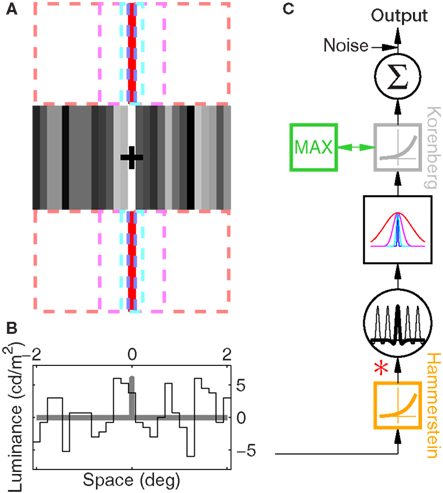
Figure 1. Experimental paradigm and computational modeling. (A) The visual stimulus consisted of 27 vertical noise bars. Observers were required to detect a fixed luminance increment applied to one of the bars (the middle one in the example here). On different blocks, one of four uncertainty regions was explicitly indicated by red uncertainty markers. The example in the figure shows uncertainty markers for the smaller uncertainty region; in this condition the markers were restricted to the size of a single bar, as indicated by the dashed blue rectangles. The remaining three uncertainty levels were indicated by markers extending to the cyan, magenta and red dashed rectangles for increasing uncertainty. (B) plots luminance values for the example shown in (A), black trace for noise and gray trace for target. Observers saw a noise-only (termed ‘non-target’) and a noise + target (termed ‘target’) stimulus on each trial; they were asked to select the interval corresponding to the target. (C) The computational models evaluated in this article represented modular versions of the block diagram shown here, i.e., they were obtained by deletions/additions of the following components: an early static non-linearity (orange square), a bank of front-end filters (big circle) applied via convolution (∗), an uncertainty window (one for each uncertainty level as shown in the big square box) applied via inner product, a late static non-linearity (gray box) or alternatively a MAX operation (green box), a simple integrator (small circle) and a late internal noise source. This cascade was applied separately to target and non-target stimuli; the stimulus associated with largest response was selected as target.
2.2 Double-Pass Experiments
We estimated internal noise (plotted on y axis in Figures 2E,F) via a double-pass methodology in which the same set of stimuli is presented twice (Burgess and Colborne, 1988). Double-pass experiments consisted of 100-trial blocks (like in the main experiment). Observers were not aware of any difference with respect to blocks for the main experiment. In double-pass blocks, the second half of the block (last 50 trials) showed the same stimuli presented during the first 50 trials, but in randomly permuted order. We collected an average of ∼1.4K ± 0.6K trials per observer. Half of these (the first 50 trials of each block) were extracted and combined with trials from the main experiment for the purpose of computing kernels. On a subset of the observers (4 out of 10) we performed additional measurements at below ( ) and above (2×) threshold SNR to determine the dependence of internal noise on stimulus intensity (Figure 2F). We collected an additional ∼3K ± 0.5K trials on average per observer for this condition. The notion of internal noise imparts a distinction between output
  defined by
  , i.e., the mean differential response to target + noise (r(s[1])) and noise-only divided by the combined SD of both external and internal (σI) noise sources, and input
  defined as
  but with σI = 0, i.e., before the addition of internal noise. The latter can be estimated, together with internal noise, from data obtained using the double-pass methodology described earlier (Burgess and Colborne, 1988; Neri, 2010a).
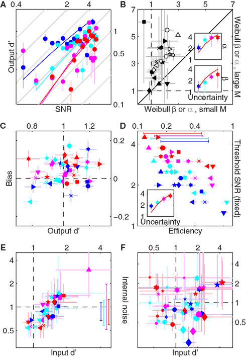
Figure 2. Performance-related metrics. (A) Aggregate psychometric curves. Colored lines show Weibull fits, gray lines indicate unity slope. (B) Best-fit Weibull parameters (threshold α (open) and slope β(solid)) for individual observers, from low uncertainty data (M = 1) on x axis versus high uncertainty (M = 27) on y axis. Insets plot averages (±SD across observers) as a function of uncertainty level (M) on x axis, red lines plot predictions from Pelli (1985) (equations 8.2–8.3 at page 1524). For β the prediction has no free parameter; for α it has 1 free parameter which we fitted (mean square error minimization). (C) Bias (y axis) versus output d′ (x axis). (D) Threshold SNR versus efficiency (square ratio between human and ideal d′). Bars next to x axis (top) show mean ± SD across observers for efficiency. Inset plots threshold SNR (which differed slightly from Weibull α, see text) as a function of uncertainty level with prediction as in inset to (B). (E) Internal noise (in units of external noise; Green and Swets, 1966) versus input d′ (see Section 2 for definition). Bars next to y axis (right) show mean ± SD across observers for internal noise (excluding observers for which estimates were >5 because deemed unreliable, see Neri, 2010a). (F) Same as (E) but including data for SNR values equal to  (smaller symbols) or 2× (larger symbols) threshold SNR. In all plots, uncertainty level is color-coded as in Figure 1A and each observer is indicated by a different symbol. Error bars show ±1 standard error of the mean (SEM) except when explicitly detailed above.
2.3 Modeling
We used variations of three main models (see Figure 1 and Theoretical Properties of MAX Kernels in Appendix): MAX (Pelli, 1985), for which the response to each stimulus s (s[1] = n + t on the target interval and s[0] = n on the non-target interval) is max(w ○ (f ∗ s)) where f is the system front-end filter, w is the intrinsic uncertainty window, ○ is Hadamard product and ∗ is convolution; Hammerstein (Hunter and Korenberg, 1986) responds 〈w, f ∗ φ(s)〉 where φ(x) = ex or φ(x) = (1 + x/n)n (which approximates ex for n→∞); Korenberg (Korenberg and Hunter, 1986) responds 〈φ(w ○ (f ∗ s)), 1〉 where φ(x) = ex (for theoretical (but not simulation) purposes we also consider φ(x) = xn, see Theoretical Properties of MAX Kernels in Appendix). The ideal model in Gaussian noise, for example, is a specific case of the Korenberg model (see Theoretical Properties of MAX Kernels in Appendix). These models were challenged with the same stimuli used for human observers and generated a binary response by selecting the stimulus interval associated with largest response (decision-variable assumption; Pelli, 1985). The corresponding kernels (Figure 5) were computed via the same analysis used for human observers (see below). We ran simulations with and without a late Gaussian internal noise source of SD equal to the SD of the model output r (average between SD of r(s[0]) and SD of r(s[1])). Figure 5 shows simulated kernels in the absence of internal noise; the addition of internal noise simply results in noisier rescaled traces (as expected). We chose to plot the noiseless results to demonstrate that the lack of second-order negative diagonal modulations for the MAX model is not due to lack of resolving power on the part of the simulations.
2.4 Kernel Computation
Estimated first-order kernels (Ahumada, 2002):  where 〈〉 is average across trials of the indexed type and Δqz = 2δqz−1. Estimated second-order kernels (Neri, 2004):
  where cov() is the covariance matrix across trials. With a number of caveats, these two operators are proportional to the corresponding first-order and second-order kernels of a Volterra expansion of the system (Neri, 2004, 2009, in press). Target-absent first-order kernels (those derived from the subset of noise fields that did not contain the target) were computed as detailed above but only for q = 0. Signal-clamped first-order kernels (Tjan and Nandy, 2006) were computed only for q = 1 and after realigning each noise trace to φ = 0 (centering the target); their centroid frequency was the mean of the corresponding power spectrum (computed via discrete Fourier transform) treated as a probability distribution (Neri, 2009). Intrinsic uncertainty windows were computed by inverse cross-correlation of first-order target-absent kernels with first-order signal-clamped kernels. Relevant mathematical properties of these kernel operators are described in the Appendix.
2.5 Consistency Estimates
Model-human consistency was computed as the percentage of trials on which the model response matched the human response; we converted it to d′ (via standard Z-score transformation, Green and Swets, 1966) because d′ units are more natural for evaluating this quantity (Neri, 2009). We tested two versions of w: Gaussian windows w(xk)[M] = 𝒩 (xk, σ[M]) where 𝒩 is the Gaussian density function with mean 0 and SD σ[M] from fit to aggregate estimate of intrinsic uncertainty windows (red line in inset to Figure 4E), and ideal windows matched to extrinsic uncertainty windows (w[M] = u[M]). When the model was parameterized on the data (e.g., f from signal-clamping, w from inverse cross-correlation, n in Hammerstein’s φ(x)) we used a  split cross-validation technique (Hong et al., 2008; Claeskens and Hjort, 2008): the data was divided into two halves; one half was used for parameterization, the other for computing consistency. We repeated the process by swapping the two halves, and used the average of the two consistency estimates. No analysis presented here used the same data for model parameterization and consistency estimation.
3 Results
3.1 Coarse Performance Metrics
Observers were required to detect a bright ‘target’ bar briefly flashed on the screen (Figure 1A) by selecting one of two successive stimulus presentations. The bar could appear anywhere within a spatial range explicitly indicated by red markers above and below the stimulus. This range was varied from block to block (indicated by dashed outlines in Figure 1A) to specify different amounts of uncertainty about target location for every block. The vertical target bar was embedded in vertical bar noise consisting of 27 additional bars whose intensity was determined by a Gaussian noise source (see Section 2 for additional details). We ran a brief set of preliminary staircase experiments to identify individual threshold SNR for all four different uncertainty levels we used (indicated by blue, cyan, magenta and red in Figure 1A). As expected from previous theoretical and experimental work on the effect of uncertainty on detectability of visual targets (Tanner, 1961; Pelli, 1985; Tyler and Chen, 2000), both the threshold point (α) and slope (β) of a Weibull fit to the psychometric curve shift to higher values as extrinsic uncertainty is increased: curves move to the right and become steeper as color coding ranges from blue to red in Figure 2A. To demonstrate the statistical reliability of this effect across observers, Figure 2B plots slope (solid symbols) and threshold values (open) for the smallest uncertainty level on the x axis versus the largest uncertainty level on the y axis; points fall clearly above the unity line (p < 0.02 for solid, p < 10−5 for open). This increasing trend applied across all four uncertainty levels (Cuzick test for trend (Cuzick, 1985) p < 0.001 for β, p < 0.02 for α) and is summarized for both α and β in the two insets to Figure 2B, showing that it is in close agreement with previous theoretical predictions (Pelli, 1985) (indicated by the red lines).
Following the preliminary assessment of threshold levels detailed above, we proceeded to collect a large number of trials (>110K) at or near the determined threshold SNR on 10 naive observers. We targeted a threshold performance level of output d′ ∼ 1 to yield near-optimal kernel quality for psychophysical reverse correlation (Murray et al., 2002), which required slight adjustments of threshold SNR in order to track learning in individual observers (compare threshold SNR determined during staircase (upper inset to Figure 2B) with those used during fixed SNR data collection (inset to Figure 2D)). We closely achieved this target as demonstrated by a scatter (SD) of only 0.2 d′ units around d′ = 1 across observers (points fall on vertical dashed line in Figure 2C, not different from 1 (p > 0.2) for any of the uncertainty levels). We were also able to avoid bias effectively (y values in Figure 2C): for the two smaller uncertainty levels bias was no different from 0 at p > 0.2 (blue and cyan symbols in Figure 2C fall on horizontal dashed line); for the two larger uncertainty levels we measured statistically significant bias in favor of the second interval (p < 0.05), but its actual value was minuscule (∼0.03 and ∼0.05 on average for the two conditions). From Figure 2C we conclude that, at least in terms of overall performance and response metrics, our observers were placed within optimal range (d′ ∼ 1, Murray et al., 2002, bias∼0, Neri, 2004, 2009).
Overall average efficiency (across conditions and observers) was 33% (±18% SD), matching the range measured by previous investigators for similar tasks (Barlow, 1978, 1980; van Meeteren and Barlow, 1981; Burgess and Barlow, 1983; Burgess and Ghandeharian, 1984a,b; Burgess, 1985; Myers et al., 1985; Burgess and Colborne, 1988; Eckstein et al., 1997), and did not differ as a function of uncertainty (Cuzick test not significant at p = 0.2; see bars near x axis (top) in Figure 2D). However we observed a significant degree of variability in how well different observers could perform the above-detailed task. Efficiency across observers spanned almost 1 entire log-unit for all uncertainty levels (x values in Figure 2D), which required the selection of SNR values spanning a fourfold range (y values in Figure 2D) in order to bring all observers within the same threshold performance range (x values in Figure 2C). This resulted in a strong negative correlation (< −0.8 for all uncertainty levels) between efficiency and threshold SNR (negative tilt in Figure 2D). We wished to pinpoint the exact source of this variability across observers, so we performed an additional set of experiments using a double-pass technique (see Section 2) that allowed independent estimation of late internal noise (y values in Figure 2E) as well as d′ in the absence of such noise (x values in Figure 2E), which we refer to as input d′ (see Section 2). When internal noise is factored out in this way, the resulting d′ values scale with threshold SNR (correlation coefficient >0.85 for all uncertainty levels, not shown) as predicted by a signal detection process with stable characteristics across observers. What is inconsistent with this simple model, however, is the result that internal noise scales with signal detectability (strong positive correlation in Figure 2E) rather than remaining constant across observers, suggesting that variability in internal noise was the main source of variability in efficiency across observers (internal noise correlates negatively with efficiency, not shown).
It should be emphasized that, although the correlation between internal noise and signal detectability demonstrated in Figure 2E renders a simple signal detection model with constant internal noise (in units of external noise) inapplicable to the entire population of observers, this does not mean that it may not apply to each observer individually. To confirm that it still applies to each observer separately, we repeated the double-pass measurements for different SNR’s applied to the same observer. As shown in Figure 2F, the strong correlation between internal noise intensity and internal signal intensity (input d′) previously measured across observers (Figure 2E) is now completely eliminated (we first computed the correlation for each observer, then applied a t-test for the resulting set of correlations being different from 0 and obtained p > 0.5 for all uncertainty levels). Figure 2F thus demonstrates that, for a given observer, internal noise intensity is constant in units of external noise intensity, in the face of large variations of signal intensity. We conclude that (similar to the popular non-linear transducer model; Nachmias and Sansbury, 1974) the most prominent source of internal noise is late, additive, and roughly equal to the intensity of the external noise source (estimates fall around 1 indicated by horizontal dashed lines in Figures 2E,F) in agreement with previous measurements of this kind (e.g., Green and Swets, 1966; Burgess and Colborne, 1988; Levi et al., 2008; Neri, 2009; see in particular Neri, 2010a for a more extensive characterization of this topic). Of particular interest is the fact that internal noise, similarly to efficiency, did not differ for the different uncertainty levels (Cuzick test p = 0.48; see bars next to y axis in Figure 2E).
The above-detailed characterization represents a necessary preliminary step for placing the data analysis and model simulations that follow within a solid framework. First, Figures 2A,B demonstrates that our methodology for manipulating extrinsic uncertainty was effective in inducing correlated shifts in intrinsic uncertainty (see also Figure 4E and related discussion later in the article), and that our experiments are immediately relevant to uncertainty as defined and examined by previous literature (Pelli, 1985; Tyler and Chen, 2000). Second, the observation that internal noise is late and independent of uncertainty simplifies modeling because it indicates that, for the purpose of a qualitative comparison between model and data, the role of internal noise is irrelevant (it only reduces the quality of our simulations as we verified directly, see Section 2). Third, while kernel estimation using psychophysical reverse correlation is reasonably well understood for late additive internal noise (Ahumada, 2002; Murray et al., 2002), the potential impact of more complex internal noise sources on this methodology has never been explored. Because many of the results described here rely on this approach, the characterization afforded by Figure 2 provides a necessary validation of the applicability of this methodology in the present context.
3.2 Estimated First-Order and Second-Order Kernels
Figure 3A shows linear (first-order) kernels derived using psychophysical reverse correlation (Ahumada, 2002) for all four uncertainty levels (different colors). As expected, their overall spatial extent reflects the corresponding level of extrinsic spatial uncertainty: the kernel corresponding to no uncertainty (blue) presents a sharp peak at target location (0 on x axis) and smaller negative side-flanks (Mexican-hat shape), while the kernel corresponding to full uncertainty (red) modulates across the whole spatial extent of the stimulus (although its amplitude is one order of magnitude smaller). We also computed full second-order (non-linear) kernels (Neri, 2004, 2009, in press) (Figures 3B–E). Because modulations within these operators occur primarily along the diagonal (variance) region, we inspect only the diagonal in Figure 3G. It is clear from a comparison between Figure 3A and Figure 3G that, to a coarse approximation, first-order kernels and second-order diagonals present similar characteristics. This observation is further emphasized by Figures 3H–K where each kernel value in Figure 3A is plotted (on the x axis) against each corresponding value in Figure 3G (on y axis). For the three smaller uncertainty levels (Figures 3H–J) first-order and second-order values covary positively (r ∼ 0.7–0.9).
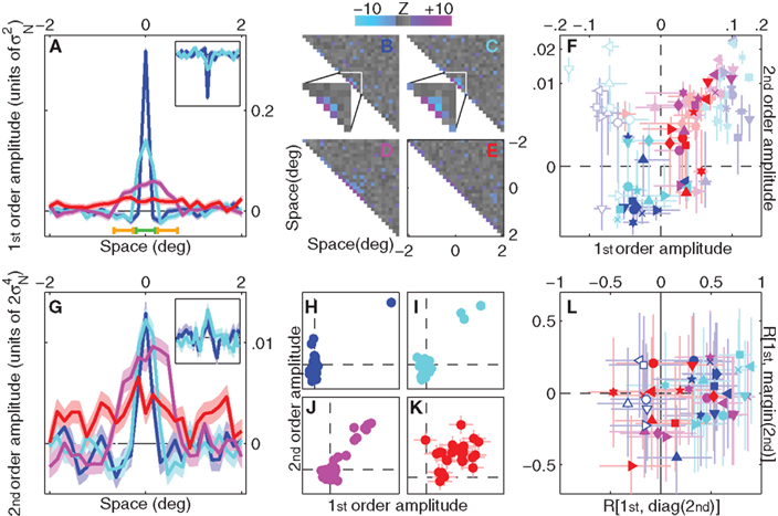
Figure 3. First-order and second-order kernels with associated metrics. (A) Aggregate first-order kernels for all 4 uncertainty levels. Inset shows first-order kernels for experiments involving detection of a dark target bar (only two uncertainty levels were tested for this condition). (B–E) Aggregate second-order kernels for the four different uncertainty levels (surface plots show Z-scores), color-coded for |Z| > 2 (red for positive, blue for negative). For the two smaller uncertainty levels (B,C) the central regions of the kernels are magnified for ease of inspection. (F) Average first-order kernel amplitude within peak range [indicated by green bar near bottom x axis in (A)] or flank range [indicated by orange bars near bottom x axis in (A)] on x axis (full color symbols for flank, light color symbols for peak), versus corresponding second-order diagonal amplitude on y axis. Solid symbols for bright target detection, open symbols for dark target detection. Axes have been warped to magnify region of interest around origin (using the map  ). (G) Aggregate second-order diagonals [same as (B–E) but only plotting the diagonal region]. Inset shows data for dark target detection. (H–K) plot each value of aggregate first-order kernels on the x axis versus the corresponding value of aggregate second-order diagonals on the y axis. (L) Correlation between first-order kernel and second-order diagonal is plotted on the x axis versus correlation between first-order kernel and second-order marginal average on the y axis, for each observer separately. Open symbols refer to dark target detection. In all plots, uncertainty level is color-coded as in Figure 1A and each observer is indicated by a different symbol. Error bars and shading show ±1 SEM.
The above-noted similarity between first-order and second-order kernels will be critical for selecting adequate computational models later in the article, making it necessary to confirm that these qualitative observations are quantitatively robust and borne out by individual observer analysis, not just by cursory evaluation of aggregate data. Because (as is normal; Meese et al., 2005) we found some variability across observers, it is difficult to draw conclusions from simply inspecting individual kernels (see Figure A1 in Appendix). We therefore performed additional analyses that captured relevant aspects of both first-order and second-order kernels, and quantified each aspect using a single value for each observer. The data could then be subjected to simple population statistics in the form of t-tests and confirm or reject specific hypotheses about the overall shape of the kernels. Our conclusions are therefore based on individual observer data, not on the aggregate observer (which is used solely for visualization purposes). This distinction is important because there is no generally accepted procedure for generating an average kernel from individual images for different observers (see Neri and Levi, 2008 for a detailed discussion of this issue).
Similarly to first-order kernels, second-order diagonals present negative modulations alongside the central positive peaks. A result of this nature, if statistically robust, would provide direct evidence against the MAX uncertainty model: this model predicts that second-order diagonals must contain only positive modulations, as we demonstrate both analytically (Theoretical Properties of MAX Kernels in Appendix) and via Monte Carlo simulations later in the article (Figure 5). Figure 3F plots kernel amplitude averaged within the peak and flank regions indicated by green and yellow horizontal bars respectively in Figure 3A. Flank values are shown in full colors, peak values in light colors, for both first-order kernels (x axis) and second-order diagonals (y axis). In line with the qualitative inspection of the aggregate data in Figure 3G, we found a significant negative modulation for the flank regions of second-order diagonal kernels from the two smaller uncertainty levels (full color blue and cyan points fall below the horizontal dashed line at p < 0.01 and p < 0.05 respectively). This effect was not significant for the two larger uncertainty levels (magenta and red), but it is not expected for these conditions (see Figure 5 and related modeling sections). Because the significant negative modulations detailed above are directly inconsistent with a MAX uncertainty model, we must conclude that this model is not applicable in the context of our experiments. Instead, these modulations are fully compatible with a different model which we detail below.
We know from well-established results in non-linear systems analysis that certain cascade models generate specific modulations within first-order and second-order kernels (Marmarelis, 2004). More specifically, we are interested here in the two most common models used in engineering and neuroscience applications: the Hammerstein NL model, where a static non-linearity precedes the linear filtering stage (Hunter and Korenberg, 1986), and the Korenberg LNL (also known as ‘sandwich’) model, where an additional front-end linear stage precedes the static non-linearity (Spekreijse and Oosting, 1970; Korenberg and Hunter, 1986) (see Section 2). The former predicts that the diagonal of the second-order kernel should have the same shape as the first-order kernel (see Theoretical Properties of MAX Kernels in Appendix), the latter makes the same prediction for the marginal average of the second-order kernel (Westwick and Kearney, 2003). We have already noted that the aggregate data appears consistent with the former prediction (Figures 3H–K). To demonstrate this result using individual observer analysis, Figure 3L plots correlation values between first-order kernels and second-order diagonals for each observer on the x axis, while the y axis plots correlations between first-order kernels and second-order marginals. Correlations with the diagonal are positive for the three smaller uncertainty levels (data points fall to the right of the vertical dashed line for blue (p < 10−5), cyan (p < 10−3) and magenta (p < 0.01)), but not for the largest uncertainty level (p = 0.98). Marginal correlations are no different from 0 for any of the four uncertainty levels (p > 0.05), indicating that modulations outside the diagonal region contained primarily noise (which eliminated the diagonal correlation; see Neri, in press for a more detailed analysis of off-diagonal modulations). We conclude that kernel structure in our experiments is consistent with the Hammerstein model, with no clear evidence that this model needs further elaboration into a Korenberg model. It is relevant in this context that the MAX model can be approximated by a Korenberg cascade (see Theoretical Properties of MAX Kernels in Appendix).
3.3 Estimation of Front-End Filtering Via Signal-Clamping
As a preliminary step toward the design of a physiologically plausible model, we will obtain an estimate of the front-end filter that is applied to the input stimulus via convolution (Figure 1C). We expect that it will be approximately similar to the first-order kernel obtained in the near-absence of spatial uncertainty (blue trace in Figure 3A), but we would like to confirm that the same filter was operating under conditions of uncertainty. This is particularly relevant here because the larger uncertainty conditions involved stimulus information from slightly more peripheral locations (up to 2° eccentricity), for which it is possible that front-end filters would be characterized by different spatial tuning. Earlier work on the application of reverse correlation techniques within regimes of uncertainty exploited a signal-clamping methodology to expose the filter underlying front-end convolution (Tjan and Nandy, 2006) (see Movshon et al., 1978 for a related application in neurophysiology). We show in “Theoretical Properties of Signal-Clamped (Target-Present) Kernels” in Appendix that this approach is only applicable within very specific conditions because it returns an estimate closer to the autocorrelation function of the front-end filter rather than the filter itself (see Figure 9). We adopt it here because the conditions of our experiments can be reasonably included within the applicable category, but it must be recognized that the interpretation of signal-clamped kernels (or the more common subclass represented by target-present kernels (Ahumada et al., 1975; Abbey and Eckstein, 2002; Neri and Heeger, 2002; Solomon, 2002; Thomas and Knoblauch, 2005)) is not straightforward.
Under signal-clamping, first-order kernels are derived from target-present noise fields contingent on target position (Tjan and Nandy, 2006) as shown in Figure 4A, where traces with lighter colors show first-order kernels for trials on which the target bar was located more peripherally. First-order kernels are now sharp-peaked for all uncertainty levels, and the peaks occur at the corresponding target locations. We used this analysis to derive front-end filters for the edge location of each uncertainty window (for the smallest uncertainty window (blue) edge and center are the same), resulting in the four black traces shown in Figure 4A (inset). All traces displayed similar tuning characteristics; to support this observation we estimated the centroid spatial frequency (see Section 2) targeted by each filter in each observer, plotted using gray symbols in Figure 4B for the smallest (x axis) versus largest (y axis) uncertainty levels. Points fall on the unity line (p = 0.2) indicating that, to a reasonable approximation, the same front-end filter operated across the entire stimulus for all uncertainty levels, a process easily implemented by straightforward convolution with one filter function. This conclusion may appear undermined by a related effect which we observed using centroid analysis: we found that when the front-end filter was estimated only for the central (foveal) location using data from the smallest as opposed to largest uncertainty conditions (x versus y axes in Figure 4B, black symbols), the latter dataset returned a lower bandpass range (black points fall below the unity line, p < 0.001). In other words, we found that the bandpass characteristics returned by signal-clamping for a given front-end filter depended not on its absolute retinal location, as one may expect from the physiologically plausible notion of a consistent bank of front-end filters, but on its location relative to the edge of the uncertainty window. However a correct interpretation of this result depends on the model supporting front-end convolution: the MAX model predicts no difference in bandpass characteristics for this analysis (green symbol in Figure 4B), inconsistent with the data; the Hammerstein model predicts that, due to the distortions introduced by the signal-clamping methodology (Theoretical Properties of Signal-Clamped (Target-Present) Kernels in Appendix), there should be an apparent difference in bandpass properties for the estimated front-end filter that matches the one observed experimentally (yellow symbol), despite no change in the underlying convolution filter itself (see Section 2). This result further corroborates the notion supported by the rest of this study that the Hammerstein model provides a simpler and more accurate account of the experimental data than the MAX model.
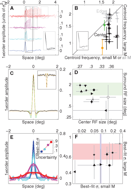
Figure 4. Signal-clamped kernels and intrinsic uncertainty windows. (A) First-order kernels (aggregate) as a function of target position for all uncertainty levels (from largest, top row, to smallest, bottom row). Lighter colors refer to more peripheral locations. Inset shows kernel averages within the four rectangular regions. (B) Centroid frequency (Neri, 2009) (in cycles/deg, see Section 2) of signal-clamped kernels for individual observers. Gray symbols refer to the edge of the extrinsic uncertainty window [same as inset to (A)], for the smaller uncertainty window on the x axis versus the largest on the y axis. For the x axis the edge is the same as the center (the smallest uncertainty window spanned one position only); because all uncertainty conditions contained the center, gray estimates on the x axis were computed from data for all four uncertainty conditions [as indicated by black rectangle in (A)]. Black symbols refer to the center of the uncertainty window, estimated from data for the smallest uncertainty condition only on the x axis versus the largest uncertainty condition only on the y axis; corresponding aggregate kernels are shown in the inset (black for data from small uncertainty condition). Green symbol shows corresponding estimate for MAX model, yellow symbol for Hammerstein (realistically parameterized in both cases). (C) Grand average of signal-clamped kernels [from all traces in (A)], black trace. Yellow trace shows DOG fit, green trace Gabor fit. Inset shows equivalent data for dark target detection. (D) Receptive field (RF) estimates from DOG fits for individual observers (center on x axis, surround on y axis), which we approximated as spanning ±2SD of the corresponding Gaussian function. Green shading shows range estimated by Shushruth et al. (2009) for 0°–2° eccentricity in macaque V1. Open symbol shows average (±SD) across observers for dark target detection. (E) Estimated intrinsic uncertainty windows (see Section 2) from aggregate data. Thick lines show Gaussian fits (mean was constrained to 0 (centered); we varied amplitude and SD). Inset plots best-fit Gaussian SD (in units of deg) on y axis as a function of uncertainty level on x axis. Line shows linear fit (in log-log axes) σ[M] = e0.6844log(M)−2.6081. (F) Best-fit Gaussian SD’s for individual observers (amplitude of fit was constrained to match peak value; fit was successful in 8 out of 10 observers), plotted on x axis for smallest uncertainty value versus y axis for largest. Shaded regions show corresponding aggregate ranges (95% confidence intervals). In all plots, uncertainty level is color-coded as in Figure 1A and each observer is indicated by a different symbol. Error bars and shading show ±1 SEM unless specified differently above.
To estimate the function for the front-end filter as effectively as possible, and to avoid committing to a specific set of assumptions at this stage, we combined all traces in Figure 4A into one trace, plotted in Figure 4C. This trace was reasonably well fitted by a difference-of-Gaussians (DOG) function, shown by the yellow line (but less well by a Gabor function, shown by the green line). The shape of this function is consistent with previous estimates of this kind (Neri and Heeger, 2002; Levi and Klein, 2002; Levi et al., 2008). To cross-check that this estimate is consistent with known facts about cortical physiology, we plot in Figure 4D both center and surround receptive field (RF) size corresponding to the best-fit DOG functions across our observers (see caption to Figure 4 for details) and compare it with the range estimated from single units in macaque primary visual cortex (Shushruth et al., 2009) indicated by the green shaded region. Overall our data falls within the expected range, suggesting that the methodology used here for retrieving the characteristics of the front-end filtering stage in the face of uncertainty is acceptable. It is worth pointing out that the front-end filter in Figure 4C is suboptimal (the optimal filter matches the target shape); this mismatch can be treated as a form of intrinsic uncertainty (not available for experimental manipulation within the context of our experiments).
3.4 Estimation of Intrinsic Uncertainty Windows
In a complementary manner to kernels derived from target-present noise fields, kernels derived from target-absent noise fields can be exploited to estimate the intrinsic uncertainty window applied by the observer to the output of the front-end convolution (Tjan and Nandy, 2006) (see Figure 1C). More specifically, the target-absent kernel reflects w ⋆ f (Theoretical Properties of Signal-Clamped (Target-Present) Kernels in Appendix); using the estimate for f derived from signal-clamping (see previous section) we can compute w via inverse cross-correlation. Figure 4E shows aggregate w estimates for the four different uncertainty levels, along with Gaussian fits (which account (overall) for 92% of the variance). Further corroborating the analysis in Figures 2A,B, the spatial extent of intrinsic uncertainty (SD of the best-fit Gaussian plotted on y axis in inset to Figure 4E) tracks the extent of experimentally imposed extrinsic uncertainty (x axis). This relationship is well fitted (p < 0.005) by a straight line in log-log axes (red line in inset to Figure 4E, see caption for details). Although in general individual observer values were scattered around the aggregate estimates (Figure 4F), we found large variability and occasionally poor reliability for Gaussian fits across observers; it is not surprising that the resolving power of our data is not robust for individual observers in relation to this specific analysis, as it involves an unusual number of preprocessing steps (signal-clamping, inverse cross-correlation, fitting). For the purpose of modeling, we therefore opted for the excellent fit to the aggregate data (red line in inset to Figure 4E) as the basis for selecting Gaussian intrinsic uncertainty windows (w). Our conclusions do not depend on this particular choice because they are either independent of the specific shape of w (for kernel-based analysis) or more generally related to the non-parametric concept of efficiency (Burgess et al., 1981) (for consistency-based analysis; see below).
3.5 Kernels Associated with Different Uncertainty Models
Figure 5 plots first-order kernels and second-order diagonals for a selection of relevant modeling schemes; when attempting physiologically plausible models we relied on the characterization detailed in the two preceding sections (see Section 2). As shown in Figures 5A,B, a straightforward implementation of the Hammerstein model returns kernel shapes that are highly consistent with those observed for the human observers, at least qualitatively. For comparison, the smaller panels show kernels obtained from a range of Korenberg/MAX cascades (we treat these two models as belonging to the same class in this article (see Theoretical Properties of MAX Kernels in Appendix for asymptotic equivalence) but it should be noted that there has been extensive effort in the literature to distinguish between specific implementations of the two (Cohn and Lasley, 1986; Klein and Levi, 2009; Solomon, 2009)). One version (panels C, E, G, and I) uses ideal uncertainty windows, the second version (panels D, F, H, and J) uses Gaussian windows (closer to human data, see Figure 4E). These additional simulations are meant to demonstrate the simple result that plausible implementations of MAX models (and Korenberg approximations to them) do not generate negative modulations within second-order diagonals; this is consistent with our theoretical prediction (Theoretical Properties of MAX Kernels in Appendix), but inconsistent with the empirical results (Figure 3). As anticipated in previous sections, we must conclude that the estimated kernels from human data support the notion that the human visual system conforms to a Hammerstein NL cascade under the conditions of our experiments, and not to a MAX model.
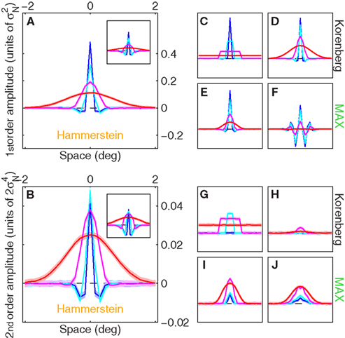
Figure 5. Kernels generated by computational models. (A) First-order kernels for Hammerstein model when realistically parameterized (Gaussian w (see Section 2), f equal to best-fit DOG to aggregate data) and n = 2. Inset shows results when φ(r) = er (i.e., n = ∞). (C) Korenberg model when ideally parameterized (w = u, f(xk) = δk0, φ(r) = er). (D) same as (C) but realistically parameterized (see above). (E) MAX model, realistically parameterized. (F) same as (E) but using f with more pronounced negative side-lobes obtained by using best-fit Gabor to aggregate data (green trace in Figure 4C) with Gaussian envelope SD set to 3×. (B,G–J) show corresponding second-order diagonals. Y axis in small panels is plotted to the same scale shown for large panels. SNR values matched human averages. For each model we ran 100 simulations (10K trials each); shading shows ±1 SD across simulations.
3.6 Trial-by-Trial Replicability of Human Responses
We can assess the applicability of different models via a completely different approach, in which we do not attempt to gauge the structure of the system, but rather focus exclusively on how well different models are able to predict whether the human observer will respond 1 or 2 on each specific trial (Neri and Levi, 2006; Neri, 2009). Figure 6 plots consistency, i.e., the percentage of trials on which two processes (e.g., human and model) give the same response to the same set of stimuli (Burgess and Colborne, 1988). This metric is closely related to the zero-one loss function used in machine learning applications (Cristianini and Shawe-Taylor, 2000; Schölkopf and Smola, 2002). Figure 6A plots model-human consistency for a physiologically plausible implementation of the Hammerstein model on the y axis, versus an equivalent implementation of the MAX uncertainty model. For these specific implementations, the latter outperforms the former when there is little uncertainty (blue and cyan symbols fall below unity line at p < 0.005 and p < 10−3 respectively), but the Hammerstein model is superior to the MAX model in the presence of substantial uncertainty (magenta and red symbols fall above unity line at p < 10−3 and p < 10−5). When spatial uncertainty is close to zero (blue) the MAX model operates like a matched template. Consistent with our results, Manjeshwar and Wilson (2001) provided fragmentary evidence that the MAX model is able to capture trial-by-trial human responses for this near-zero uncertainty condition, but its predictive power collapses as soon as the smallest amount of spatial uncertainty is introduced.
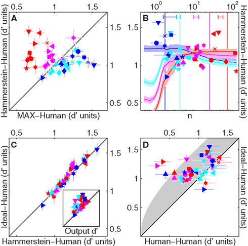
Figure 6. Trial-by-trial response consistency between human and model. (A) Model-human consistency (% of trials on which the human observer and the model gave the same response to the same set of stimuli, converted to d′ units; Neri, 2009) for MAX (realistically parameterized) on the x axis, versus Hammerstein (realistically parameterized with φ(r) = er) on the y axis. (B) Smooth lines show how model-human consistency for Hammerstein model (realistically parameterized, plotted on y axis) varies as a function of n (specifying the expansive nature of the early non-linearity φ(r) = (1 + r/n)n) on x axis. Shading shows ±1 SD across observers. Symbols show, for each observer, the n value (on x axis) associated with largest consistency (on y axis). Bars near x axis (top) show mean ± SD of these n values. Vertical lines show the n value associated with highest efficiency (maximizing % correct) averaged across observers. (C) Model-human consistency for the ideal observer (y axis) versus the Hammerstein model (realistically parameterized) with n matched to values indicated by symbols in (B). Inset plots same on y axis, versus d′ on x axis; the latter is the model-human consistency expected of a hypothetical model (not realizable for the SNR values used in our experiments) that selects the target interval on every trial (Neri, 2009). (D) same as (C) on y axis, versus human-human consistency on x axis (human self-replicability) estimated from double-pass experiments (Burgess and Colborne, 1988) (see Section 2). Gray-shaded region shows range for highest consistency theoretically possible (Neri and Levi, 2006). Error bars show ±1 SEM unless specified differently above. Except for x axis of (B), axes of all other panels are in d′ units (not %).
Clearly, model-human consistency depends on the exact parametrization used for the model. As an example, Figure 6B shows how model-human consistency varies as a function of the power exponent (n) for the early non-linearity in the Hammerstein model: larger values of n (x axis) correspond to a more expansive non-linearity (n = 1 is linear). Interestingly, we observed a trend whereby the n value associated with largest model-human consistency (indicated by symbols for individual observers) was close to squaring in the absence of uncertainty (average x value for blue symbols is 2.1 ± 0.9 SD across observers), but increased in the presence of uncertainty (red symbols are shifted to the right of blue symbols, p < 0.005), meaning that the best-fit early non-linearity becomes more pronounced as uncertainty is increased. When the non-linearity in the Hammerstein model is matched to the average best-fit exponent from Figure 6B (via cross-validated procedure), this model performs as well as the MAX model for the smaller uncertainty conditions (while remaining superior for larger uncertainty) and approaches the consistency afforded by the ideal observer model. This is shown in Figure 6C, where ideal consistency is plotted on the y axis versus consistency for the above-detailed implementation of the Hammerstein model: there is no difference for all uncertainty levels (p > 0.05). This result is consistent with the noteworthy observation that the n value that maximizes target detection (largest d′), indicated by vertical lines for the different uncertainty levels in Figure 6B, also increases with uncertainty in a manner similar (although not identical) to the trend observed for the n value that maximizes model-human consistency (bars near top x axis). In other words, it appears that the early non-linearity is adjusted to maximize performance under different levels of uncertainty.
Despite the inability of the ideal observer to capture the kernel structure observed experimentally (Figures 5C,G), we consistently found an improvement in model-human consistency as different models were modified to approach the ideal observer model. Indeed, model-human consistency for the ideal observer (and for the optimized Hammerstein model detailed earlier) was well within the maximum range theoretically possible. Figure 6D plots consistency for the ideal observer on the y axis (same as y axis in Figure 6C) versus human-human consistency, i.e., the percentage of trials on which the human observers gave the same response to two presentations of the same visual stimulus (this quantity was estimated using the double-pass procedure described earlier in the article). Human-human consistency can be used to determine an expected region for the best achievable consistency by any model (Neri and Levi, 2006; Neri, 2009), shown by gray shading in Figure 6D. Consistency values for the ideal observer are mostly within this region. Surprisingly, they are significantly greater than human-human consistency for almost all uncertainty levels (blue, magenta and red symbols fall above unity line (p < 0.05) but not cyan (p = 0.13)). Such high predictive power is rarely observed at threshold (compare with Neri, 2009).
The analysis presented in Figure 6 leads to the conclusion that the ability of different models to replicate human trial-by-trial responses in the conditions of our experiments may be assessed by determining their efficiency, i.e., how closely they approach the ideal observer (Green and Swets, 1966; Burgess et al., 1981) (this is not always the case, see Neri, 2009 for a counter-example). In this sense, model-human consistency falls within the category of coarse metrics (e.g., d′) that do not allow a clear distinction between the inefficient ideal observer and other models (see Section 1). When combined with the kernel-based analysis detailed earlier, however, the above conclusion prompts a closer evaluation of how robust different models can be under varying degrees of realistic parameterization; we examine this issue below.
Figure 7 plots efficiency for the two models of interest in this study: the MAX model on the y axis, versus the Hammerstein model on the x axis. When the front-end filter is ideal (i.e., a delta function) and the intrinsic uncertainty windows are ideal (i.e., they match the spatial range for target position), the Hammerstein model is identical to the ideal observer and the MAX model is nearly identical to it for all uncertainty levels (indicated by symbol size) as demonstrated by the blue circles in the upper-right corner (and as theoretically expected, see Theoretical Properties of MAX Kernels in Appendix). A more realistic implementation involves Mexican-hat shaped front-end filters that mimic the one derived from human data (Figure 4C). Red symbols refer to the empirically estimated best-fit DOG filter. It is clear that, under this type of realistic front-end filtering, the MAX model is more efficient than the Hammerstein model when uncertainty is small (small circles fall above unity line), but worse when uncertainty is large (large symbols fall below unity line). As the front-end filter is made to depart even more from the ideal filter by broadening its tuning characteristics (yellow and green symbols), this trend is preserved but it becomes apparent that the Hammerstein model is far more robust than the MAX model in conditions where the front-end filter is badly matched to the signal: efficiency values barely change for the Hammerstein model (red, yellow and green traces are aligned vertically), while they drop significantly for the MAX model (red, yellow and green traces are increasingly shifted downwards). As the next step of approximation to a realistic implementation is afforded by using Gaussian uncertainty windows (black symbols) rather than ideal boxcar windows, the efficiency range spanned by the Hammerstein model falls within the range estimated for a noiseless human observer (gray solid and dashed boxes) while the MAX model falls outside this range when uncertainty is large, and is very inefficient (∼0.2). We conclude from Figure 7 that, within the constraints imposed by the characteristics of realistic human visual filters and uncertainty weighting functions, the MAX model is not sufficiently robust to represent a viable choice except when uncertainty is very small. In contrast, the Hammerstein model is resilient to these limitations.
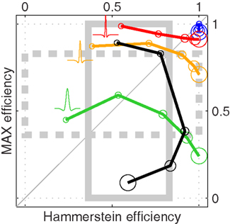
Figure 7. Efficiency (square ratio to ideal d′; Green and Swets, 1966) of MAX (y axis) versus Hammerstein (x axis) models. Symbol size indicates uncertainty level (3j−1 for j = 1 to 5). Blue symbols refer to ideal parameterization; red symbols to f matching best-fit DOG to aggregate data (Figure 4C), yellow symbols to same f but stretched along the x axis (broadened) by 2×, green symbols by 3×, black to same f as for red but Gaussian w instead of ideal w. Each symbol shows mean of 100 simulations (5K trials each). Gray rectangles indicate efficiency range for human input d′ (see Section 2), mean ± SD across observers (dashed for y axis).
3.7 Exclusion of Potential Role for Stimulus Artifacts
The early non-linearity we characterized in the previous sections is suspiciously reminiscent of the expansive non-linearity that is commonly observed for uncalibrated monitors: when pixel intensity is controlled linearly at the palette level, the actual output from the monitor is typically supralinear (Brainard et al., 2002). Is it possible that our experiments exposed this non-linearity in the stimulus hardware, rather than in the observer’s visual system? We took great care in gamma-correcting our monitor to eliminate this non-linearity altogether, but we wished to further exclude a potential role for such an artifact by collecting more data based on the following logic. As detailed earlier, the Hammerstein model predicts a correlation between the first-order kernel and the second-order diagonal (see Theoretical Properties of MAX Kernels in Appendix); the sign of the correlation is determined by the first-order and second-order coefficients in the Taylor expansion of the early non-linearity (Westwick and Kearney, 2003; Neri, 2009). If the target bar is made dark, the appropriate Hammerstein model would apply a non-linearity where the sign of the first-order coefficient is opposite to that used for a bright target bar. We therefore expect that, in conditions where observers are asked to detect a dark bar, the resulting kernels would show a negative correlation between first-order kernels and second-order diagonals. More specifically, we expect that first-order kernels would be a sign-inverted version of those obtained for detecting a bright bar, while second-order kernels would remain unchanged (see Theoretical Properties of MAX Kernels in Appendix). If, on the other hand, the early non-linearity derives from monitor miscalibration, the characteristics of this non-linearity will not change, leaving the sign of the correlation between first-order kernels and second-order diagonals unchanged.
We tested these predictions by performing additional measurements for the two smaller uncertainty levels on a subset of the observers (see Section 2), who were presented and asked to detect a dark rather than a bright bar. The results were unequivocal: first-order kernels inverted their sign (inset to Figure 3A), but not second-order kernels (inset to Figure 3G). Individual observer analysis confirmed these trends: peak amplitude was significantly negative for first-order kernels but positive for second-order diagonals (open symbols fall within second quadrant in Figure 3F, p < 0.05), and the correlation between first-order kernel and second-order diagonal was significantly negative for the smallest uncertainty level (open blue symbols in Figure 3L are shifted to the left of the horizontal dashed line at <10−3; we were not able to measure a statistically significant effect for the other uncertainty level tested). We also estimated the front-end filter for these experiments, which looked very similar to the filter for detecting a bright target (inset to Figure 4C) and fell within the expected physiological range (open symbol in Figure 4D shows average across observers). We conclude from this analysis that the early non-linearity we described previously exists in the brain of the observers, not in the monitor.
4 Discussion
Uncertainty has been a subject of controversy on a number of occasions in the vision literature (Cohn and Lasley, 1986; Klein and Levi, 2009). The debate has focused primarily on whether uncertainty is involved in specific phenomena such as dipper effects (Solomon, 2009) or stochastic resonance (Perez et al., 2007), not on how it operates: once it is agreed that uncertainty is present, there is widespread consensus that visual detection relies on a late MAX operation (Pelli, 1985; Klein and Levi, 2009) to the extent that the two terms ‘uncertainty model’ and ‘MAX model’ are often treated as synonyms and used interchangeably in the vision literature (Klein and Levi, 2009; Solomon, 2009). Our study does not speak to the debate over the presence/absence of uncertainty: we deliberately inject uncertainty into the experiments, control its extent explicitly, and confirm that the classic signatures of its presence (Pelli, 1985; Tyler and Chen, 2000) apply to our data (Figures 2A,B). Our study is concerned with the question of how visual processing operates under uncertainty when it is present, and it challenges the notion that it is supported by a MAX model, at least for the specific task and stimuli adopted here. The main feature of the model we favor, known as Hammerstein (Hunter and Korenberg, 1986; Marmarelis, 2004), is the presence of an early non-linearity. Below we discuss a few issues that are directly relevant to this stage in the model.
4.1 Characterization and Interpretation of the Early Non-Linearity
Throughout this report we have drawn a distinction between the NL Hammerstein model and the LNL Korenberg model. However it is evident that in general the former represents a subclass of the latter (Marmarelis and Marmarelis, 1978; Marmarelis, 2004): insertion of an early convolution with a delta function before the static non-linearity leaves the output unchanged, but turns the NL model into an LNL model. How can our data reject LNL models, and at the same time accept NL models which are also LNL models? This result is a consequence of the specific way in which the models are formulated to encompass sensible implementations of uncertainty models (Figure 1). In the L1NL2 implementation of a MAX uncertainty model, the linear stage L2 immediately preceding the psychophysical decision is necessarily a simple sum (this stage (indicated by Σ in Figure 1C) does not even exist in the MAX model as the max operation already returns a single decision variable (Pelli, 1991)). Both front-end filtering and weighting by the intrinsic uncertainty window (indicated by large circle and large square boxes respectively in Figure 1C) are lumped into the early linear stage L1 (see Section 2). As discussed in detail earlier (and demonstrated in Theoretical Properties of MAX Kernels in Appendix) this formulation is incompatible with the modulations we observed in the second-order kernels (Figure 3). In the Hammerstein model, the linear stage immediately preceding the psychophysical decision corresponds to L1 (front-end convolution followed by weighting), not L2; formally adding an early (ineffective) linear stage does not therefore reduce it to the LNL implementation of a MAX model. The prediction for the Hammerstein model is consistent with the data (Figure 5). To summarize, our conclusions can only be understood in relation to the specific formulation of cascade models that is necessary to accommodate uncertainty, not in general with relation to any Hammerstein/Korenberg cascades.
The issue of formulating the front-end stage in the Hammerstein model draws attention to a further question: what is a plausible physiological substrate for this stage? As mentioned in the preceding paragraph, there is an implicit assumption in this model that the earliest stage involves a high-fidelity linear transducer (a delta function); a compatible physiological interpretation would presumably place this stage at retinal or geniculate level. The subsequent early non-linearity may then reflect the rectifying properties of ON and OFF channels (Shapley, 2009) in line with previous psychophysical work claiming a role for these non-linearities in pattern vision (Bowen, 1995), and more specifically in relation to effects often attributed to uncertainty (Bowen, 1997). However these considerations are highly speculative at this stage, and arguably incompatible with a number of details reported here, for example the indication in Figure 6B that the properties of the non-linearity may be task- dependent, a characteristic that would not be generally associated with pre-cortical processing. Our model is therefore best interpreted as an abstract formulation of the underlying mechanisms, which also makes it potentially applicable to a wider range of problems (see Section 4 below) and to existing literature. For example, a similar model has been considered by Kontsevich and Tyler (2002), Abbey and Eckstein (2006); more specifically, Abbey and Eckstein (2006) found that it was able to explain aspects of their data unaccounted for by a MAX uncertainty model. It is also interesting that a critical feature of the MIRAGE model (Morgan and Watt, 1997) is an early, highly non-linear channeling of stimulus information into ON and OFF pathways; the non-linearity is applied to each spatial scale after linear filtering, but it interacts with the linear stage in a more fundamental way than in other general models of spatial vision.
If we are not positioned to relate these models to specific physiological constructs, can we at least sketch an intuitive description in terms of the associated phenomenological experience? We attempt this in Figure 8 where MAX (left) and Hammerstein (right) models are reduced to minimal cartoon-like descriptions, for the specific purpose of offering an intuitive understanding of what these models actually mean in relation to the perceptual process. The input stimulus presented in the first interval is shown alongside (separated by ‘vs’) the stimulus presented in the second interval (bottom of figure); for the example shown here the target interval is second. In the MAX model (left) each stimulus is converted to an image where only the brightest bar within that stimulus is preserved (lefthand pair of stimuli); the two brightest bars from the two stimuli are then compared and the brighter is chosen (this decisional process is indicated using the ≶ notation borrowed from Pelli, 1985). In the Hammerstein model (right) each stimulus is warped to emphasize its ‘bright-bar’ content, i.e., relatively bright regions are made brighter while relatively dark regions are made less dark (righthand pair of stimuli); evidence from all regions within each stimulus is then combined (Σ) to contribute a figure of merit for that stimulus, and the final decision is generated by comparing outputs from the two stimuli. It is clear that, although the two models share some similarities, they differ in important respects and imply distinct perceptual strategies.
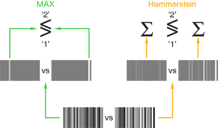
Figure 8. Cartoon-like descriptions of MAX (left) and Hammerstein (right) models. The two input stimuli are shown at the bottom (separated by ‘vs’); the target increment was added to the second stimulus. The MAX model selects the brightest bar within each stimulus (lefthand pair of stimuli) and compares the two outcomes from the two stimuli to reach a final decision, which is ‘1’ if the brightest bar in the first stimulus is brighter than the brightest bar in the second stimulus, ‘2’ if the other way around (this process is indicated by the ≶ symbol). The Hammerstein model operates differently: the two input stimuli are subjected to a static non-linearity (ex) whereby the ‘bright-bar’ content of each stimulus is emphasized (righthand pair of stimuli) before summing the evidence across the entire stimulus (Σ) to obtain a final figure of merit for comparison/decision (≶).
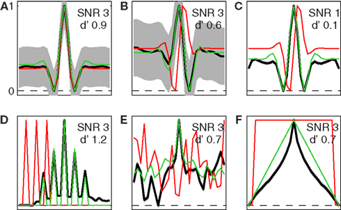
Figure 9. Simulated signal-clamped kernels for MAX model. Uncertainty range u extended to entire x axis (w = u, M = 27). Red traces show true front-end filter f ((A) even Gabor, (B,C) odd Gabor, (D) pulse sequence, (E) Gaussian noise sample, (F) wide boxcar function), black traces show signal-clamped estimates (shading ±1 SD over 100 simulations of 100K trials each), green trace shows f * f + f * f2 except for panel C where it only shows f * f (this term is expected to play a more prominent role at low SNR, see Theoretical Properties of Signal-Clamped (Target-Present) Kernels in Appendix). All traces have been rescaled so that their minimum value equals 0 and their maximum value equals 1. SNR used for the simulation (with corresponding model d′) is indicated in each panel separately.
4.2 Robustness of the Hammerstein Model
If we accept the notion that human observers were striving to maximize efficiency within the constraints imposed by early filtering in the visual system and suboptimal encoding of the specified target uncertainty ranges (as indicated by the high model-human consistency achieved by the ideal observer in Figures 6C,D), then the Hammerstein model represents a more robust choice than the MAX model. Figure 7 demonstrates that the former is highly resilient to suboptimal processing by physiologically plausible hardware, while the latter is unable to retain a viable level of efficiency when uncertainty is large. The constraints imposed by neural hardware are likely more pronounced in natural vision. In the conditions of our experiments, observers were presented with a visual stimulus and task they knew close to everything about: its appearance, exact target characteristics, explicit uncertainty range, timing. For example, because they knew the spatial scale of the stimulus and the bars within it, their visual system could rely on the subset of spatial channels with tuning characteristics roughly matched to the bars. This is unlikely in natural vision, where the front-end filter may be significantly mismatched to the target. Our simulations indicate that the MAX model is not robust against this type of suboptimality, while the Hammerstein model is (compare red, yellow and green traces in Figure 7). It is interesting that recent studies of SNR response properties in single neurons have demonstrated how early non-linearities (as early as the rod-rod bipolar synapse (Field and Rieke, 2002)) can play a critical role in sensory processing of noise-corrupted signals (Field et al., 2005), as well as serve functional roles previously attributed to non-linear operations happening much later in the processing hierarchy (Carandini et al., 2002; Read et al., 2002; Rosenberg et al., 2010).
There are other features of the Hammerstein model that make it potentially more attractive than the MAX model. It is conceivable that it can be implemented more easily in neural hardware: static non-linearities are ubiquitous in neural structures and arise naturally from well-known properties of neuronal physiology (Priebe and Ferster, 2008). Furthermore, they are instantaneous. MAX operations are commonly implemented via winner-take-all algorithms (Pelli, 1991), but these take time to converge when applied to realistic network settings (Wilson, 1999). Finally, the structure and analysis of the Hammerstein model merge naturally with current theory and knowledge. For example, it is known that under ideal conditions the MAX model approximates the ideal observer; but under ideal conditions (and for the class of target signals used here) the Hammerstein model is formally identical to the ideal observer (Theoretical Properties of MAX Kernels in Appendix; see also Figure 7). Ideal observer analysis is a fundamental branch of signal detection theory and psychophysics (Green and Swets, 1966), making the Hammerstein model theoretically attractive. More importantly, its properties are well-known (Marmarelis and Marmarelis, 1978) particularly in relation to reverse correlation techniques and predicted kernel structure (Westwick and Kearney, 2003; Marmarelis, 2004).
4.3 Max or Hammerstein?
The experiments described in this paper are restricted to a specific task, that of detecting a luminance bar embedded in noise. Although pertinent to visual processing and perhaps representative of a larger class of problems in visual detection, it is clearly inadequate as a proxy for more complex tasks. Suppose for example the task involves selecting, of two crowds, the crowd containing a specific target face. If we adopt a template-matching strategy, all faces in the stimulus must be matched against a template (or set of templates) for the target face. The MAX model applies seamlessly to this scenario, whereas the Hammerstein model is possibly undefined in this case: the static non-linearity must be applied before template matching, but what does it mean to apply a point-non-linearity to a whole face? Applying this kind of transformation to individual pixels in the image would make no sense for the task at hand.
This problem may be alleviated by recasting it in terms of feature space (a common strategy in kernel methods; Schölkopf and Smola, 2002): the input space, consisting of face pictures, is transformed into a ‘face’ space, where each face maps to a low-dimensional vector (Lee et al., 2000). It may then make sense to apply the early static non-linearity within feature space (an operation for which there is some experimental evidence, see Dakin and Omigie, 2009). In the case of the task described earlier, each face would map to a space whose axes represent for example eye-shape, mouth-width, beard-density, and mustache-size. To detect Karl Marx’s face, an expansive non-linearity would be applied to the beard-density and mustache-size axes in order to emphasize their impact on the final sum across all features and faces within each crowd (an operation not too dissimilar from automated caricature generation; Lee et al., 2000). A relevant consequence of this formulation is that, in order to test different models using the tools described in this article, it would be necessary to apply noise in feature space and reverse correlate that space. Whichever approach is taken, many more experiments than those presented here are necessary to determine whether the Hammerstein model, which we have shown to outperform a number of other models in the specific case of a simple visual detection task, also represents a valid alternative to the highly successful MAX model in relation to visual processing in general.
Conflict of Interest Statement
The author declares that the research was conducted in the absence of any commercial or financial relationships that could be construed as a potential conflict of interest.
Acknowledgments
Supported by Royal Society (University Research Fellowship) and Medical Research Council (New Investigator Research Grant).
References
Abbey, C. K., and Eckstein, M. P. (2002). Classification image analysis: estimation and statistical inference for two-alternative forced-choice experiments. J. Vis. 2, 66–78.
Abbey, C. K., and Eckstein, M. P. (2006). Classification images for detection, contrast discrimination, and identification tasks with a common ideal observer. J. Vis. 6, 335–355.
Ahumada, A. J. (2002). Classification image weights and internal noise level estimation. J. Vis. 2, 121–131.
Ahumada, A. J. Marken, R., and Sandusky, A. (1975). Time and frequency analyses of auditory signal detection. J. Opt. Soc. Am. A Opt. Image Sci. Vis. 57, 385–390.
Barlow, H. B. (1978). The efficiency of detecting changes of density in random dot patterns. Vision Res. 18, 637–650.
Barlow, H. B. (1980). The absolute efficiency of perceptual decisions. Philos. Trans. R. Soc. Lond. B Biol. Sci. 290, 71–82.
Bowen, R. W. (1995). Isolation and interaction of ON and OFF pathways in human vision: pattern–polarity effects on contrast discrimination. Vision Res. 35, 2479–2490.
Bowen, R. W. (1997). Isolation and interaction of ON and OFF pathways in human vision: contrast discrimination at pattern offset. Vision Res. 37, 185–198.
Brainard, D. H., Pelli, D. G., and Robson, T. (2002). Display characterization. Encycl. Imaging Sci. Technol. 172–188. Available at: http://color.psych.upenn.edu/brainard/characterize.pdf
Burgess, A., and Barlow, H. B. (1983). The precision of numerosity discrimination in arrays of random dots. Vision Res. 23, 811–820.
Burgess, A. E. (1985). Visual signal detection. III. On Bayesian use of prior knowledge and cross correlation. J. Opt. Soc. Am. A 2, 1498–1507.
Burgess, A. E., and Colborne, B. (1988). Visual signal detection. IV. Observer inconsistency. J. Opt. Soc. Am. A 5, 617–627.
Burgess, A. E., and Ghandeharian, H. (1984a). Visual signal detection. II. Signal-location identification. J. Opt. Soc. Am. A 1, 906–910.
Burgess, A. E., and Ghandeharian, H. (1984b). Visual signal detection. I. Ability to use phase information. J. Opt. Soc. Am. A 1, 900–905.
Burgess, A. E. Wagner, R. F., Jennings, R. J., and Barlow, H. B. (1981). Efficiency of human visual signal discrimination. Science 214, 93–94.
Carandini, M., Heeger, D. J., and Senn, W. (2002). A synaptic explanation of suppression in visual cortex. J. Neurosci. 22, 10053–10065.
Claeskens, G., and Hjort, N. L. (2008). Model Selection and Model Averaging. Cambridge: Cambridge University Press.
Cohn, T. E., and Wardlaw, J. C. (1985). Effect of large spatial uncertainty on foveal luminance increment detectability. J. Opt. Soc. Am. A 2, 820–825.
Cristianini, M., and Shawe-Taylor, J. (2000). Support Vector Machines. Cambridge: Cambridge University Press.
Dakin, S. C., and Omigie, D. (2009). Psychophysical evidence for a non-linear representation of facial identity. Vision Res. 49, 2285–2296.
Eckstein, M. P., Ahumada, A. J., and Watson, A. B. (1997). Visual signal detection in structured backgrounds. II. Effects of contrast gain control, background variations, and white noise. J. Opt. Soc. Am. A Opt. Image Sci. Vis. 14, 2406–2419.
Field, G. D., and Rieke, F. (2002). Nonlinear signal transfer from mouse rods to bipolar cells and implications for visual sensitivity. Neuron 34, 773–785.
Field, G. D., Sampath, A. P., and Rieke, F. (2005). Retinal processing near absolute threshold: from behavior to mechanism. Annu. Rev. Physiol. 67, 491–514.
Franz, M. O., and Schölkopf, B. (2006). A unifying view of wiener and volterra theory and polynomial kernel regression. Neural Comput. 18, 3097–3118.
Hong, X., Mitchell, R. J., Chen, S., Harris, C. J., Li, K., and Irwin, G. W. (2008). Model selection approaches for non-linear system identification: a review. Int. J. Syst. Sci. 39, 925–946.
Hunter, I. W., and Korenberg, M. J. (1986). The identification of nonlinear biological systems: Wiener and Hammerstein cascade models. Biol. Cybern. 55, 135–144.
Klein, S. A., and Levi, D. M. (2009). Stochastic model for detection of signals in noise. J. Opt. Soc. Am. A Opt. Image Sci. Vis. 26, B110–B126.
Kolmogorov, A. N., and Fomin, S. V. (1957). Elements of the Theory of Functions and Functional Analysis. Rochester, NY: Graylock Press.
Kontsevich, L., and Tyler, C. W. (2002). A single-channel model for spatio-temporal contrast sensitivity at low-to-medium spatial frequencies. J. Vis. 2, 6a.
Korenberg, M. J., and Hunter, I. W. (1986). The identification of nonlinear biological systems: LNL cascade models. Biol. Cybern. 55, 125–134.
Lasley, D. J., and Cohn, T. E. (1981). Why luminance discrimination may be better than detection. Vision Res. 21, 273–278.
Lee, K., Byatt, G., and Rhodes, G. (2000). Caricature effects, distinctiveness, and identification: testing the face-space framework. Psychol. Sci. 11, 379–385.
Levi, D. M., and Klein, S. A. (2002). Classification images for detection and position discrimination in the fovea and parafovea. J. Vis. 2, 46–65.
Levi, D. M., Klein, S. A., and Chen, I. (2008). What limits performance in the amblyopic visual system: seeing signals in noise with an amblyopic brain. J. Vis. 8, 1–23.
Manjeshwar, R. M., and Wilson, D. L. (2001). Hyperefficient detection of targets in noisy images. J. Opt. Soc. Am. A Opt. Image Sci. Vis. 18, 507–513.
Marmarelis, P. Z., and Marmarelis, V. Z. (1978). Analysis of Physiological Systems: The White-Noise Approach. New York: Plenum Press.
Marmarelis, V. Z. (2004). Nonlinear Dynamic Modeling of Physiological Systems. Piscataway, NJ: Wiley IEEE Press.
Meese, T. S., Hess, R. F., and Williams, C. B. (2005). Size matters, but not for everyone: individual differences for contrast discrimination. J. Vis. 5, 928–947.
Morgan, M. J., and Watt, R. J. (1997). The combination of filters in early spatial vision: a retrospective analysis of the MIRAGE model. Perception 26, 1073–1088.
Movshon, J. A., Thompson, I. D., and Tolhurst, D. J. (1978). Receptive field organization of complex cells in the cat’s striate cortex. J. Physiol. (Lond.) 283, 79–99.
Murray, R. F., Bennett, P. J., and Sekuler, A. B. (2002). Optimal methods for calculating classification images: weighted sums. J. Vis. 2, 79–104.
Murray, R. F., Bennett, P. J., and Sekuler, A. B. (2005). Classification images predict absolute efficiency. J. Vis. 5, 139–149.
Myers, K. J., Barrett, H. H., Borgstrom, M. C., Patton, D. D., and Seeley, G. W. (1985). Effect of noise correlation on detectability of disk signals in medical imaging. J. Opt. Soc. Am. A 2, 1752–1759.
Nachmias, J., and Kocher, E. C. (1970). Visual detection and discrimination of luminance increments. J. Opt. Soc. Am. 60, 382–389.
Nachmias, J., and Sansbury, R. V. (1974). Letter: grating contrast: discrimination may be better than detection. Vision Res. 14, 1039–1042.
Neri, P. (2010b). Stochastic characterization of small-scale algorithms for human sensory processing. Chaos (in press).
Neri, P., and Heeger, D. J. (2002). Spatiotemporal mechanisms for detecting and identifying image features in human vision. Nat. Neurosci. 5, 812–816.
Neri, P., and Levi, D. M. (2006). Receptive versus perceptive fields from the reverse-correlation viewpoint. Vision Res. 46, 2465–2474.
Neri, P., and Levi, D. M. (2008). Evidence for joint encoding of motion and disparity in human visual perception. J. Neurophysiol. 100, 3117–3133.
Pelli, D. G. (1985). Uncertainty explains many aspects of visual contrast detection and discrimination. J. Opt. Soc. Am. A 2, 1508–1532.
Pelli, D. G. (1991). “Noise in the visual system may be early,” in Computational Models of Visual Processing, eds M. Landy and A. J. Movshon (Cambridge, MA: MIT Press), 147–152.
Perez, C. A., Cohn, T. E., Medina, L. E., and Donoso, J. R. (2007). Coincidence-enhanced stochastic resonance: experimental evidence challenges the psychophysical theory behind stochastic resonance. Neurosci. Lett. 424, 31–35.
Peterson, W. W., Birdsall, T. G., and Fox, W. C. (1954). The theory of signal detectability. IRE Trans. Inf. Theory 4, 171–212.
Priebe, N. J., and Ferster, D. (2008). Inhibition, spike threshold, and stimulus selectivity in primary visual cortex. Neuron 57, 482–497.
Read, J. C., Parker, A. J., and Cumming, B. G. (2002). A simple model accounts for the response of disparity-tuned V1 neurons to anticorrelated images. Vis. Neurosci. 19, 735–753.
Rosenberg, A., Husson, T. R., and Issa, N. P. (2010). Subcortical representation of non-Fourier image features. J. Neurosci. 30, 1985–1993.
Shapley, R. (2009). Linear and nonlinear systems analysis of the visual system: why does it seem so linear? A review dedicated to the memory of Henk Spekreijse. Vision Res. 49, 907–921.
Shushruth, S., Ichida, J. M., Levitt, J. B., and Angelucci, A. (2009). Comparison of spatial summation properties of neurons in macaque V1 and V2. J. Neurophysiol. 102, 2069–2083.
Solomon, J. A. (2002). Noise reveals visual mechanisms of detection and discrimination. J. Vis. 2, 105–120.
Spekreijse, H., and Oosting, H. (1970). Linearizing: a method for analysing and synthesizing nonlinear systems. Kybernetik 7, 22–31.
Tanner, W. P. (1961). Physiological implications of psychophysical data. Ann. N. Y. Acad. Sci. 89, 752–765.
Thomas, J. P., and Knoblauch, K. (2005). Frequency and phase contributions to the detection of temporal luminance modulation. J. Opt. Soc. Am. A Opt. Image Sci. Vis. 22, 2257–2261.
Tyler, C. W., and Chen, C. C. (2000). Signal detection theory in the 2AFC paradigm: attention, channel uncertainty and probability summation. Vision Res. 40, 3121–3144.
van Meeteren, A., and Barlow, H. B. (1981). The statistical efficiency for detecting sinusoidal modulation of average dot density in random figures. Vision Res. 21, 765–777.
Victor, J. D. (2005). Analyzing receptive fields, classification images and functional images: challenges with opportunities for synergy. Nat. Neurosci. 8, 1651–1656.
Watson, A. B., and Ahumada, A. J. (2005). A standard model for foveal detection of spatial contrast. J. Vis. 5, 717–740.
Westwick, D. T., and Kearney, R. E. (2003). Identification of Nonlinear Physiological Systems. Piscataway, NJ: Wiley IEEE Press.
Keywords: non-linear kernel, volterra expansion, reverse correlation, visual psychophysics
Citation: Neri P (2010) Visual detection under uncertainty operates via an early static, not late dynamic, non-linearity. Front. Comput. Neurosci. 4:151. doi: 10.3389/fncom.2010.00151
Received: 15 February 2010;
Accepted: 10 November 2010;
Published online: 30 November 2010.
Edited by:
Stefano Fusi, Columbia University, USAReviewed by:
Bosco Tjan, University of Southern California, USAGabriel Kreiman, Harvard University, USA
Denis Pelli, New York University, USA
Copyright: © 2010 Neri. This is an open-access article subject to an exclusive license agreement between the authors and the Frontiers Research Foundation, which permits unrestricted use, distribution, and reproduction in any medium, provided the original authors and source are credited.
*Correspondence: Peter Neri, Institute of Medical Sciences, Aberdeen Medical School, Aberdeen, UK. e-mail:cGV0ZXIubmVyaUBhYmRuLmFjLnVr