 Dana H. Ballard1* and Janneke F. M. Jehee2
- 1 Department of Computer Science, University of Texas at Austin, Austin, TX, USA
- 2 Donders Centre for Cognitive Neuroimaging, Nijmegen, Netherlands
A prominent feature of signaling in cortical neurons is that of randomness in the action potential. The output of a typical pyramidal cell can be well fit with a Poisson model, and variations in the Poisson rate repeatedly have been shown to be correlated with stimuli. However while the rate provides a very useful characterization of neural spike data, it may not be the most fundamental description of the signaling code. Recent data showing γ frequency range multi-cell action potential correlations, together with spike timing dependent plasticity, are spurring a re-examination of the classical model, since precise timing codes imply that the generation of spikes is essentially deterministic. Could the observed Poisson randomness and timing determinism reflect two separate modes of communication, or do they somehow derive from a single process? We investigate in a timing-based model whether the apparent incompatibility between these probabilistic and deterministic observations may be resolved by examining how spikes could be used in the underlying neural circuits. The crucial component of this model draws on dual roles for spike signaling. In learning receptive fields from ensembles of inputs, spikes need to behave probabilistically, whereas for fast signaling of individual stimuli, the spikes need to behave deterministically. Our simulations show that this combination is possible if deterministic signals using γ latency coding are probabilistically routed through different members of a cortical cell population at different times. This model exhibits standard features characteristic of Poisson models such as orientation tuning and exponential interval histograms. In addition, it makes testable predictions that follow from the γ latency coding.
1 Introduction
Although individual visual cortical neurons exhibit deterministic spiking in special instances, e.g., during sleep cycles (Drestexhe and Sejnowski, 2001), for the most part they exhibit predictably random spiking behavior that can be modeled closely as a Poisson process (Softky and Koch, 1993) with baseline rates that have been shown to correlate with experimental parameters in hundreds of experiments. Because of this extensive data set, it often is taken for granted that a neuron’s basic function is to communicate a scalar parameter by the spike rate. Nonetheless there is reason to be dissatisfied with this stance. Typical firing rates of individual cells are low, in the range 10–100 Hz, whereas motor responses to visual stimuli in the form of saccades can be as fast as 100 ms (Kirchner and Thorpe, 2006). This means that the communication of rate is unrealistically slow if it depends on individual cells. For this reason the classical approach to explain how fast behavioral responses are possible has used population codes (e.g., Georgopoulos et al., 1986; Averbeck et al., 2006; Chen et al., 2006) that interpret the combined output of large numbers of cells as a faster and more accurate signal. However, using a substantial number of cells with each communicating the same unary code also seems unsatisfactory (Softky, 1990, 1996). In the first place, population codes can be expensive in terms of the number of synapses required to support them. Even for modest precision and confidence in estimating an analog value such as rate, over a 100 synapses can be required for a single input (see The Cost of Precision in a Rate Coding Model in the Appendix). Secondly, spikes can be expensive metabolically. In one estimate, spike generation and transmission consume nearly half of a cell’s metabolism when all the costs are taken into account (Attwell and Laughlin, 2001; Lennie, 2003).
Specialized interpretations of the spike code have been made, for example that action potentials literally signal Bayesian statistics (Ma et al., 2006). In contrast, our hypothesis is that the cortex’s cell firing patterns comprise a more rapid generic message sending strategy that can appear Poisson at the single cell level. We describe such a way that the cortex may use timing in spike codes, that has advantages for both understanding signaling as well as cortical plasticity. Most importantly, our code can reproduce experimental “rate” measurements.
Sparse Coding Models of Cortical Cells
A general way that cortical neurons can be characterized is in terms of their receptive fields. Collections of these can be interpreted mathematically as a library of functions, termed basis functions, that can encode any signal in terms of a sum of pairwise products of the basis functions and associated coefficients. Thus, a vector of sensory or motor data values distributed over a space x, I(x), may be approximated with N such functions using:

A basis function specified by the vector ui(x) represents the synapses comprising the receptive field of the i-th neuron, and the scalar ri is a coefficient, or strength, that that cell should signal. The simplicity of Eq. 1 belies a fundamental implication of this model and that is that the component cells’ spikes must be used in two different tasks simultaneously, each having different requirements. Spikes must firstly be used to help a cell learn its receptive field by adjusting the strength of its synapses, and secondly communicate the coefficient that codes the receptive field’s portion of the stimulus. These two tasks have radically different information processing requirements. A cell’s receptive field exhibits long-term plasticity and the synapses that compose it are continually being adjusted (Bonomano and Merzenich, 1998; Sanes and Donoghue, 2000). This task is slow and incremental, occurring prominently during development, but also in adulthood, and uses aggregates of inputs. In contrast, signaling via spikes occurs vary rapidly in the course of responding to a stimulus and typically uses just a few spikes over a very fast 100∼300 ms timescale. Equation 1 indirectly specifies both of these tasks. If the input is an ensemble of data samples {I}, the plasticity task is to learn a set of basis functions {u}. However, if these basis functions are fixed, as they are assumed to be on short time scales, then the task is quickly to signal a specific input via an appropriate set of coefficients {r}.
Tremendous progress has been made in developing mathematical formulations that solve both of these problems in a way that explains biological features, such as the orientation distributions of simple cells in striate cortex, by adding a term to Eq. 1 that penalizes solutions that use many non-zero coefficients (Rao and Ballard, 1996; Olshausen and Field, 1997; Lewicki and Sejnowski, 2000; Bell and Sejnowski, 2003; Rehn and Sommer, 2007). The crucial idea is that, in order to minimize some cost, such as metabolic energy, the cortex develops many more coding cells that the minimum necessary, so that for any particular stimulus, a small set of cells with basis functions specialized for that stimulus suffices. This minimal coding strategy is referred to as the sparse coding principle and having a surfeit of coding cells characterizes the population as being overcomplete. Although the main modeling demonstrations illustrating these points have been in the circuitry connecting the lateral geniculate nucleus to striate cortex, as we do here, the results are indicative of a much more general principle that may extend to all of cortex (Rao and Ballard, 1999).
The sparse coding results are important, but so far the majority of models have used abstractions of neurons with signed real numbers for outputs, which in turn assume some kind of population coding, instead of directly dealing with action potential spikes. The crucial issue is: if the cortex is to use a minimal number of spiking cells, how are they to communicate analog values? There have been several ingenious methods to do so by exploiting timing codes (Eliasmith and Anderson, 2003; Eliasmith, 2005; Joshi and Maass, 2005; Lazar, 2010), but these methods may be challenged in the cortex if several independent computations may be simultaneously active (von der Malsburg, 1999). Another possibility is to use a rank order code (Perrineta et al., 2004), or its variant, a latency code (Shaw, 2004). These methods work for feed forward circuits. However, for the cortex’s ubiquitous feedback circuits, one needs a more general system that has a common timing reference (e.g., Zhang and Ballard, 2004).
A γ Frequency Model
One possible timing resource is the cortex’s rhythmic signals in the γ range (30–80 Hz). It has been suggested that the cortex might use an analog latency with respect to the phase of a γ frequency oscillatory signal to do this (Buzsáki and Chrobak, 1995; Fries et al., 2007) and recent evidence is in support of this (Vinck et al., 2010). This coding strategy is very different from the standard Poisson-based population models. Latency temporal coding (Delorme et al., 2001; Gollisch and Meister, 2008), when referenced to a γ timing signal, allows a single spike to communicate an analog quantity in a way that is interpretable by both feed forward and feedback circuitry. As a further consequence, small subsets of cells can represent a stimulus adequately and, crucial to our model, the overcompleteness of cortical representations means that many different subsets of cells can communicate the same stimulus. Of course, population codes also use different subsets of cells in signaling but the latency codes turn out to need orders of magnitude less cells to achieve equivalent precision and confidence levels.
Another important consequence of a latency code is that it is compatible with spike timing dependent plasticity (STDP; Bi and Poo, 1998). STDP specifies that the learning rule for a cell is a function of a timing reference. Although the original experiments used the timing of a cell’s output spike as a reference, the STDP rule could in principle apply to an extracellular reference as assumed here. Since STDP effects are based on latencies, a latency code is a straightforward way of meeting this requirement.
We have proposed a specific model based on γ latencies (Jehee and Ballard, 2009). This model proposes that γ latencies serve as a general base representation for communicating analog values in both feed forward and feedback pathways. However, our initial studies using this model to learn and use receptive fields abstracted away important issues related to representing individual spikes, such as a detailed model of latency and the latency code spike statistics. The focus of this paper is to address these issues with an explicit spike model in a circuit of significant scale. In this paper we show, via a number of specific simulations, how the γ latency code can serve as a general coding strategy and, at the same time, can exhibit statistics in individual cells that are very close to those of a Poisson model.
The key testable predictions of the model concern properties of the latency coding of spikes. If the stimulus is represented by a latency code, many repeated applications of the same stimulus, on average, should result in the reuse of the same latencies. Thus, the distribution of latencies in any neuron, measured with respect to the γ timing phase, should be highly non-uniform. This prediction is in direct contrast to that of a Poisson model, which would predict a uniform distribution that is independent of any particular γ reference. A subtler prediction involves the fundamental constraint between the spikes of neurons with overlapping receptive fields. If only one spike from the overlapping group is sent, then the groups’ spikes should not be correlated at short (1∼3 ms) timescales. If more than one spike is sent during that period, the component latencies would have to have been adjusted accordingly. Neurons with non-overlapping receptive fields can be correlated, and in fact should be, as the representation of stimuli is still distributed across multiple cells, albeit in much smaller groups than needed by rate-code models.
2 Methodology
The development of neural receptive fields in the striate cortex has received extensive study and has become a standard venue for testing different neural models. Thus, this circuitry provides an ideal demonstration site for our very different model of cortical neuron coding and signaling. The more abstract version of the algorithm has been shown to learn receptive fields in cortical areas V1 and MST (Jehee et al., 2006) as well as to account for temporal feedback effects from striate cortex to the LGN (Jehee and Ballard, 2009). The basic core of the algorithm is recapitulated in Section “The Algorithm for Learning Receptive Fields” in the Appendix. Here we describe the modifications for keeping track of individual spikes.
What makes the model fundamentally different is its combination of three interlocking constraints: (1) randomized action potential selection, (2) variable γ latency coding, and (3) multiplexing of several different γ range frequencies.
2.1 Randomized Action Potential Selection
A central constraint on action potential generation concerns neurons with overlapping receptive fields. Two receptive fields are said to overlap when the dot product of their normalized receptive fields is significant, which we take to be greater than some scaler value μ. In our simulations most neurons are nearly orthogonal, that is, the dot product is less than 0.20. Rather than selecting the most similar neuron at each instant, neurons with significantly overlapping receptive fields compete to be chosen (Jehee et al., 2006). In terms of the spike model, when two basis functions overlap significantly, they are as a consequence not orthogonal and must probabilistically compete to be the one chosen to send a spike as shown in Figure 1. The probability of being chosen is given by p = e10r/Z where r is the projection, the empirically determined scalar 10 weights the largest responders, and Z is a normalization factor. In the figure the red circles denote the two competing responses of the left and right receptive fields for a particular input. The probabilistic protocol is dictated by the expectation maximization constraint (Dempster et al., 1977) for estimating overlapping probability distributions. Its absence leads to double counting that results in erroneous receptive fields. Our claim is that the observed randomness in spike trains may be a consequence of the need to satisfy this constraint, which ensures that receptive fields are learned correctly.
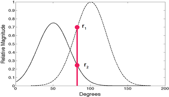
Figure 1. Random action potential spike selection. On each γ cycle, only one of neurons with overlapping receptive fields can signal. Whether or not a neuron sends an action potential is determined probabilistically according to the relative projections of the input onto receptive fields. For the two neuron example shown, for the particular input shown in red, the odds of the leftmost neuron being chosen over the rightmost neuron is given by the ratio of r2 to r1. In the case of multiple overlapping receptive fields, the odds are distributed appropriately among them.
2.2 Gamma-Latency Coding
A general way that all cells can signal coefficient information is via γ latencies, as shown in Figure 2. Each spike communicates numerical information by using relative timing (Kirchner and Thorpe, 2006; Gollisch and Meister, 2008) where in a wave of spikes the earlier spikes represent higher values. This strategy can be used in general circuitry, including feedback circuitry, if such waves are referenced to the γ oscillatory signal (Fries et al., 2007). Spikes coincident with zero phase in the γ signal can signal large numbers and spikes lagging by a few milliseconds can signal small numbers. The particular formula we use to relate the projection r to latency l is given by

where l is the latency value in milliseconds and α is a constant that has value 0.9 at 50 Hz.
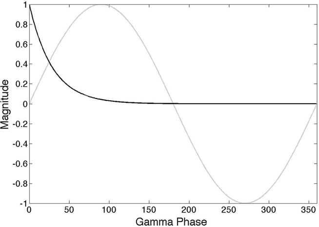
Figure 2. γ latency code. The action potential of a neuron encodes an analog value in terms of a latency(black curve) that is scaled with respect to the phase of a particular γ frequency (gray curve). The model assumes that several different subnetworks can be simultaneously active and that they are each distinguished by using a frequency in the γ range.
The assumption of the ubiquitous use of latency coding is that it allows numerical data to be propagated throughout the relevant cortical circuitry quickly and, at the same time, owing to the sparseness of the code, makes this circuitry relatively insensitive to cross-talk from any other spike traffic. Given a set of learned receptive fields, an input stimulus initially can be represented by selecting a candidate probabilistically from amongst the set of V1 neurons that have receptive fields that are similar to the input, subtracting the candidate’s receptive field from the input, and repeating this process with the resultant residual acting as a new input. The specific algorithm to do this has been described in (Jehee et al., 2006), and is based on matching pursuit (Mallat and Zhang, 1993). After k basis functions (neurons) have been selected, the input from the LGN has been reduced to

where  is the latency of neuron in.
A key assumption in the model concerns the mechanism for realizing this equation in neural circuitry. The use of γ latency coding to represent quantities suggests that the process of evaluating residuals should be done in one or two γ cycles. Otherwise it would take too long to represent the input stimulus. For example, since each cycle consumes on the order of 20 ms, if it took a cycle for each of 10 coefficients, the total time budget would be unrealistic. Thus, our model posits that an essential role of lateral connections in V1 is to implement the subtraction process shown in Eq. 3 for each of the N different component basis functions within one or two cycles, and the particular simulations herein assume all the subtractions are done within a single γ cycle. This is a temporarily demanding constraint, nonetheless the requisite circuitry is in place to do this (e.g., Martinez et al., 2005). There is not a huge wealth of data showing how rapidly cells can communicate in situ, but (Crapse and Sommer, 2009), show that the superior colliculus can cause spikes in the frontal eye fields within 1–2 ms. Thus one would expect that local communication within a cortical area might take considerably less time.
Another important constraint is that, in order to be latency coded without error, the residual magnitudes need to be generated in decreasing order. This is usually the case as highly overcomplete representations mean that some neuron’s receptive field is close to the residual and thus has a high probability of being chosen. This probability can also be tuned by scaling β in Eq. 10.
Learning the receptive fields starting from random connections is straightforward. At each step, the winning neuron has its receptive field made a little more similar to that of the stimulus that resulted in its selection. This can be done by moving each receptive field in the direction of its residual, i.e., the k-th receptive field changes by

where η is a scalar learning rate.
This equation shows that the learning of receptive fields can take place simply using STDP if both use the same latency code. Since (1) Δu ∝ ΔI, (2) the former is signaled by latencies with respect to the γ phase, and (3) both the model and experimental data use exponential decreases (Bi and Poo, 1998), the adjustment is in principle straightforward.
2.3 γ Frequency Band Multiplexing
The γ band is a broad range and consequently it would be unlikely to expect a single frequency to be chosen and used as a “clock.” Indeed elaborate statistical tests for such a clock in local cortical field potential data over 2–4 s have been negative (Burns et al., 2010). However, it may very well be the case that the cortex can have multiple simultaneous computations that each use a separate oscillatory frequency in the γ range. Indeed there are reasons to suspect that this is possible. As noted by (Ray and Maunsell, 2010), the observed γ frequency scales with contrast, so at least the oscillatory frequency can be adjusted. Consequently, we assume that the latency code can be adjusted to reflect the particular frequency used. To handle this we scale the value of α by each frequency i.e.,

where γo is assumed to be 50 Hz. The assumption of multiple frequency latency codes potentially allows multiple independent sets numerical data to be propagated throughout the relevant cortical circuitry quickly and, at the same time, owing to the sparseness of the code, makes this circuitry relatively insensitive to cross-talk from any other spike traffic.
3 Results
The focus of our simulations is to show that timed circuits that use the randomized spike generation protocol send information in a very different way than is currently conceived in that the group of cells sending the information varies from cycle to cycle. However, despite this difference, the spikes in this code can appear to be very similar to those generated by a Poisson processes. At the same time, the latency code introduces regularities in the spike distributions with respect to the γ phase that should be detectable.
γ Latency Coding Produces Conventional Orientation Tuning Curves
Does this process generate data that describes conventional receptive fields? We tested the claim that rival neurons were competing in simulation. Neurons whose receptive fields were learned with the matching pursuit algorithm that used the conventions of our model were tested on an 8 × 8 simulation by using small Gabor image patches as input. The Gabor patches were computed using the parameters (wavelength, phase offset, bandwidth, aspect ratio) = (2, 0, 1, 1). The wavelength is measured in pixels.
Thirty-six Gabor image patches were created, one for every 10° rotation. These were then presented to the network 1200 times and fit with learned basis functions each time. To emphasize the point that the randomized neural selection process models the receptive field, we chose two basis functions that overlap and measured their receptive fields using their spike counts for the different Gabor orientations. Their histogram data are indicated in Figure 3. The spike counts, which in the model reflect the number of times they were chosen probabilistically, are representative of standard oriented receptive fields measured experimentally using repeated trials to generate a post-stimulus time histogram, even though the model’s process for generating spikes is very different from any standard rate-code model.
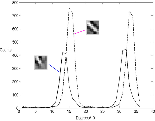
Figure 3. The orientation tuning of the γ latency code shows the classical bell-shape tuning. The histogram of two 8 × 8 receptive fields learned by the algorithm tested with a rotated set of Gabor patches 10° apart. Each histogram records, for 1200 presentations at each tested orientation, the number of times the neuron was randomly selected by the algorithm. By way of comparison, in a conventional model the y-axis would record the match between the input and the receptive field. The two peaks for each neuron result from the fact that the Gabor patch is self similar every 180°.
Simulations Showing the Random Routing of the Signal
The Gabor image test shows that a probabilistic selection method can produce orientation tuning but does not show off two crucial features of the coding method, namely (1) the codings of an image patch vary from γ cycle to γ cycle and (2) they use latency coding to send a coefficient. These two features are made explicit in Figure 4. In this larger 10 × 10 simulation the same image patch is fit repeatedly with 12 basis functions for 200 times. The simulation essentially assumes that there is no underlying time constant linking one fitting iteration to the next, i.e., the circuit is assumed to be memoryless. However, by adapting the method of (Druckmann and Chklovskii, 2010), memory could be added.
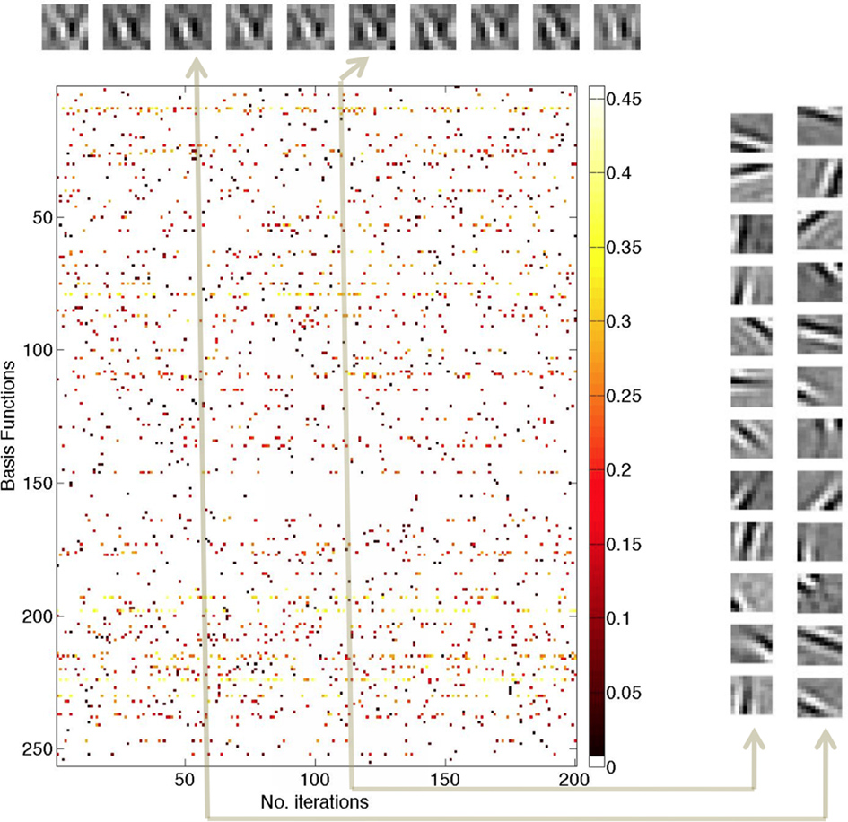
Figure 4. Responses of 256 model neurons when re-coding a single 10 × 10 image patch repeatedly for 200 γ cycles. (Top) Invariant encoding. The reconstruction of the input patch for cycles 20, 40, 60, 80, 120, 140, 160, 180, and 200. At each update cycle, the reconstruction of the image input patch changes slightly but is for the most part invariant. (Center) Individual spikes communicate numerical values by virtue of their latency relationship to a γ phase. Owing to the probabilistic nature of cell selection, at each cycle, different neurons are selected and send a spike. The latency of each spike is denoted by a color that encodes its scalar coefficient. The highest values are light yellow to white and lowest values are dark red. These values are translated into milliseconds using the latency formula in Eq. 2. (Right) Basis functions for two coding cycles Cycles 60 (1200 ms) and 120 (2400 ms) are representative examples showing that the sets of 12 neurons sending spikes vary from update to update.
The simulation uses 256 neurons and shows the spikes for each of 200 γ cycles, representing 4 s of elapsed time (200 × 20 ms). Each colored dot represents a spike for a particular neuron and in each column 12 such spikes are present, 1 from each of 12 neurons selected. The spikes are color-coded to indicate their γ latency values, with light yellow to white being the highest value and dark red being the lowest. The colored scale bar indicates the values of the coefficients prior to latency conversion. Neurons that are used frequently have high coefficient values.
The 10 inset images in a row at the top of this figure are reconstructed from the sum of products of the 12 coefficients at cycles {20, 40, 60, 80, 100, 120, 140, 160, 180, 200} and these images show a high degree of invariance despite the fact that the basis functions used in encoding the patch are different. For example, comparing the basis functions for cycles 60 and 120 (shown on the extreme right hand side) shows that the neurons used to represent the patch are almost entirely different. This can be checked visually by picking a receptive field for the 60 ms patch encoding and trying to find its counterpart in the 120 ms patch encoding and vice versa.
One direct consequence of the probabilistic spike selection strategy is that if the individual neurons are examined, their spike “rate” is correlated with their average response coefficients. Here we use “latency code” as a synonym for “response” since a recipient neuron can decode the latencies to recover the responses. To demonstrate this feature, Figure 5 plots, for each neuron, the sum of its responses (coded as latencies) against the number of times it was chosen. This rate-latency code correlation is one reason why it could be difficult to appreciate a latency code as the basis for neural signaling. Since latency code is correlated with the spike rate, the rate suggests itself as the primary signaling code, whereas, under the latency hypothesis, the rate is just a byproduct of a more efficient timing-based code.
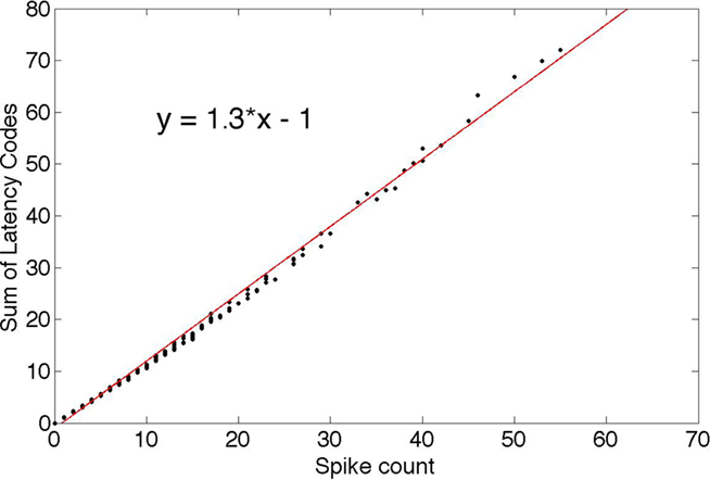
Figure 5. The sum of the latencies sent by the neurons is correlated with their spike rate.
The data in Figures 4 and 5 plot only the spikes coding the stimulus. No competing stimuli are present and there are no noise effects. However, it is unreasonable to expect that a population of neurons would be isolated in this way. To that end, we conducted two additional simulations in successively more realistic environments.
Poisson Model Comparison: Modeling the Background as Noise
In the first test, we constructed a more complete spike data set by embedding those spikes in a “noise bath” of background neural spiking. The idea of noise here is as a model for any other ongoing processing. For each neuron, the probability of firing at each millisecond was set to 0.008, representing approximately 10 Hz background rate, and the model’s spikes were added to this bath. For comparison, we compared these spike trains to a pure noise bath with firing probability of 0.01. The different background rates were chosen so that the number of spikes in each case was approximately the same. The results are shown in Figure 6. The black curve shows the cumulative distribution of the spike train for the spikes that use random routing plotted against the cumulative distribution for white noise spikes. By way of comparison, the red curve shows the distribution of spikes in a case where random routing is not used and one set of coefficients is simply repeated, plotted against the cumulative node distribution. It is easily seen that the random routing necessitated by the learning algorithm obscures the timing signal. With the random routing, no timing perturbation is noticeable even after 40 s of simulation. In contrast, without the random routing constraint, the effect of the γ latency code clearly shows up in the plot as a step change, representing the influence of the highly detectable 50 Hz signal.
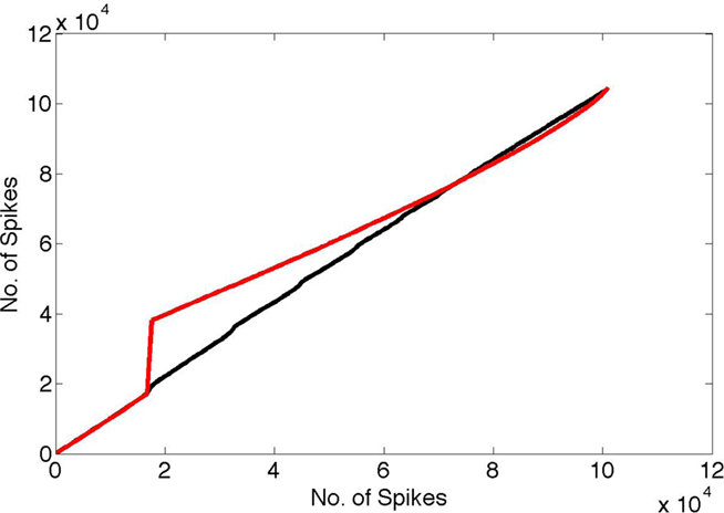
Figure 6. Spike interval histograms were computed for both the pure noise bath and the noise bath with the code embedded in it under two conditions. In one random routing was used to select the coefficients, and in the other the same coefficients were re-sent at each coding cycle. Next the cumulative density functions (cdfs) of these two cases (vertical axis) were plotted against the cdf for a pure noise bath of the same number of spikes (horizontal axis). Note that if two cdfs were identical the result would be a straight line. The γ timing signal clearly shows up using the cdf for the case where the same coefficients are used at every cycle (red curve) vs. the random cdf. In contrast, the random routing cdf vs. the random cdf tends to obscure the γ signal completely (black curve).
Poisson Model Comparison: Spike Interval Histograms of Multiple γ Processes
The test shown in Figure 6 provides an additional indication that the γ latency code can appear similar to a random spike code but at the same time there are more exacting tests than the cumulative distribution comparison. Also, the overcompleteness measure of 2.56 is not very representative of the cortex, which uses overcompleteness measures greater than 10. To attempt to approximate this larger overcompleteness ratio, we resorted to using copies of the learned basis functions in a more exacting test. Basis sets of 512 (×2) and 768 (×3) were constructed by replicating the original learned set. With a larger set, the spike rates for individual cells decrease, so that, to bring the rates up to biologically observed levels, multiple different patch codings were used. For the case of the ×2 set 12 patches were coded, and for the case of the ×3 set, 18 patches were coded. Note that this is possible owing to the enormous economies introduced by the γ latency code which uses sparseness to ameliorate cross-talk. In addition, per (Diesmann et al., 1999), a baseline noise rate of 2 Hz was added to each spike train.
An issue that has been finessed up to this point is that γ frequencies appear in a range of 30–80 Hz. Thus per (Ray and Maunsell, 2010), for the proposed strategy to work, the latency code has to be sensitive to the particular frequency chosen. As a consequence, it could be assumed that multiple encodings are using different frequencies. Therefore, for the different simultaneous encodings, it is assumed that they each can use a different frequency in the γ range, and this is modeled by choosing random frequencies with wavelengths in the range [20 ± (no. patches)/2]. In addition an initial phase offset for each coding in the range [0, 20] is chosen. Finally, the appropriate latency for each neuron’s coefficient is added as an offset to its γ reference.
Figure 7 shows the comparison of γ latency encodings with one set of random spike trains (Figure 7A) whose level of randomness has been adjusted to make the total spikes similar to those in the γ latency spike trains. All the comparisons use 1 ms resolution. The simulations lasted for 4 s, or approximately 200 γ intervals. We assume that the different patch encodings are not confused, since they use different phases and offsets and the spike trains are very sparse. For each graph, five different runs are made and the data combined in a interval histogram plot with the standard error in the mean at each sample denoted by color. Figure 7B shows that for the overcompleteness ratio of 7.68, the interval histogram is very similar to that observed in purely random spike data. Similarly for the overcompleteness ratio of 5.12, the histogram is very similar to the random plot. However, when the ratio is reduced to 5.12, and the γ range is also restricted to 50 ± 1 Hz, the effects of γ timing clearly can be seen; however, one must appreciate that this test is severe, as the encodings are designed to be similar, 512 cells are used, and the measurement interval is 4 s. Furthermore, experimental measurements of larger numbers of cells using local field potentials regularly show a γ signal.
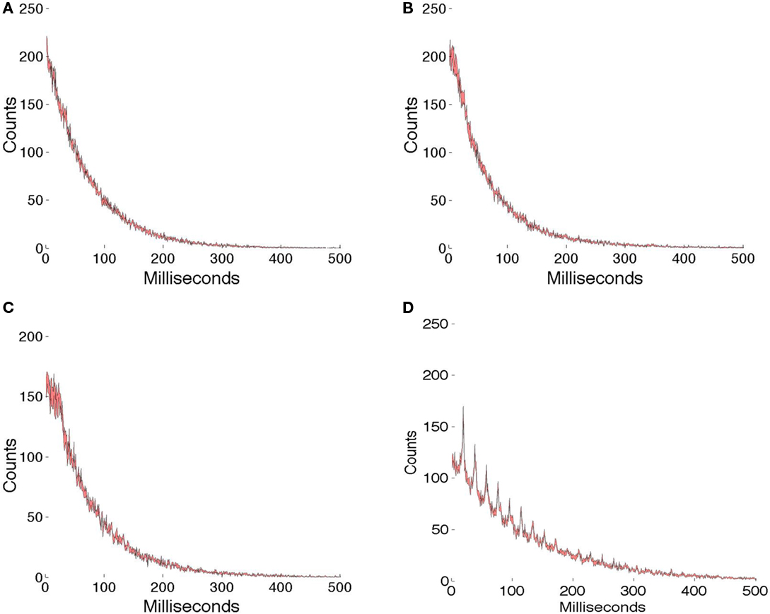
Figure 7. Interval histograms. (A) Spikes chosen randomly with a probability that equalizes the total number of spikes used in the γ latency coding. (B) 256 × 3 basis functions used to code 18 image patches (see text). (C) 256 × 2 basis functions used to code 12 image patches. (D) 256 × 2 basis functions. When the γ signal is restricted to a small range (50 ± 1 Hz), it can be clearly seen. For each data set spike interval histograms are computed at 1 ms resolution. The color is used to indicate the SE of the mean value for five runs.
Testable Hypothesis
Figure 8 shows an essential feature that would distinguish the model from a standard Poisson model. If the same image patch is used repeatedly, then any given neuron will have, on average, a discrete set of coefficients that it signals, owing to the discrete nature of the signaling pool of cells. Thus, if a histogram is made of these coefficients for each cell, as is shown in the figure, the entries will not be uniform, as expected if the process were Poisson, but instead will exhibit the asymmetries shown, where certain latencies are used much more frequently than others.
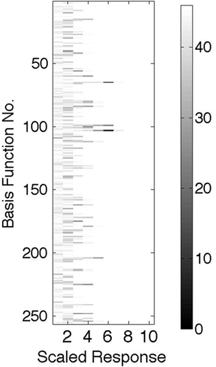
Figure 8. For each basis function the scaled and quantized histogram of latencies is plotted where the number of coefficients of a given latency range is represented by a gray scale with the scale calibration on the RHS. This example shows, contrary to a Poisson expectation, that the distribution is very non-uniform.
4 Discussion and Conclusions
Our primary hypothesis is that the rate code observed in so many experiments might be an abstraction of a more fundamental and efficient latency code that uses frequencies in the γ range as timing references but can generate rate-like statistics when tested by conventional means. This stands in contrast to models that posit that rate codes and γ frequency codes are separate and compatible (e.g., Masuda and Aihara, 2003). The particular γ latency code model tested in simulation here combines both probabilistic selection and multiplexing and has several important features.
1. Large scale computation It specifies a way of organizing computations that span different areas throughout the cortex that is impervious to other ongoing computations. The neurons that are tied to a specific γ frequency can communicate with each other easily. Cross-talk with other action potentials is minimal owing to the sparseness of the representations and the different γ frequencies. Potentially, a given neuron can participate in several different computations, each one specified by a particular γ frequency.
2. Generic signal representation It is generic in that the signal representation can suffice for any analog quantity, so that different algorithms that the cortex might use can be interfaced without any difficulty.
3. STDP compatibility The use of the latency code by the learning algorithm is of significant interest since it exploits precisely the timing feature used in STDP (Bi and Poo, 1998). Found in the hippocampus, the learning time constants are about three times longer than needed to support learning in our model, where changes are communicated within 5 ms windows, but it may turn out that STDP is faster in the cortex. Certainly to take full advantage of γ latency coding it needs to be. In such a coding the modulation of learning in models such as ours scales the magnitude of the effects in precisely the way signaled by the delay code.
4. Poisson-like statistics It can reproduce the Poisson-like statistics that are the hallmark of rate-code models. From this perspective, the post-stimulus histogram is useful as a correlate of the putative γ latency code.
However the γ latency code is not without challenges. It is significantly more technically demanding to implement than the standard rate code and the following issues need to be addressed in future work that would use a more detailed neural model.
1. Precision How much precision can one expect in the action potential? Our model assumes that the action potential peak is the key indicator. Given a 5- to -10 ms latency window, four bits of precision would require the ability for the recipient neuron to discriminate peaks that are as small as 0.25–0.5 ms apart. This would seem very demanding. However, an ameliorating factor is that since just the receptive field response is to be estimated and this estimate appears as the form of a weighted average, an additional three bits of information may be possible by the action of accumulating charge at the soma.
2. Spike Random selection and communication We do not specify exactly how the spikes are generated, and to do this places demands on the neuron. There has to be a mechanism that translates the differences in potential into a probability, and, at the same time, uses this information in the coding of latency. In addition, once selected, the neuron has to communicate its value rapidly to the other neurons in the pool. Our basic assumption is that the size of the pool has to be less than the axonal branching factor which is usually assumed to be on the order of 104.
3. Sequentiality The associated matching pursuit learning algorithm has an inherent sequentiality that is demanding to model, however our simulations assume that this sequentiality can be integrated into the generation of the γ phase codes. This process is technically demanding: the largest component must remove its components so that they are not party to the choice of larger γ latencies representing smaller magnitudes. In that way, all the component neurons can be found in one γ cycle. This is possible as the axonal propagation speeds in myelinated sensory neurons are on the order of 5∼25 m/s. Another option is that, as long as neurons with substantial overlap can compete, the process can be conducted in parallel. The consequence is that the result can be off by a scale factor, but there maybe ways of fixing this result. Future work will address this option.
4. Decoding Another challenge for γ latency coding is that of decoding. Consider the task a recipient neuron faces in recognizing a coded image patch. The code can be realized in many different ways as shown in Figure 4. However a straightforward way of decoding would be to connect the appropriate basis functions’ axons to the decoding neuron’s dendritic tree. Given that the recipient neuron can have on the order of 10,000 synapses and on the order of 10 basis functions are used per code, ideally 103 slots would be available. To reduce cross-talk, it may be possible to organize all the connections for any given code on the same branch of the dendritic tree.
5. Phase locking A final implementation issue for the underlying biology is to realize different frequencies in the γ range. We envision that the lower levels in the cortical mantle can do this and that the result is somehow mapped onto the pyramidal circuitry that is doing the main processing and thus cells in a large network can be quickly synchronized. Other studies have suggested ways of doing this.
When phase locked, the γ latencies may be difficult to detect. We envision that the temporal usefulness of a particular set of γ latencies might be as little as 300 ms, the typical time used to acquire information with a saccade and commensurate with the times used in visual routines (Roelfsema et al., 2003). Furthermore it may be possible that many simultaneous such routines could coexist, each using a γ signal with a different global phase. Both of these possibilities, together with the random routing constraint, combine to make the detection of the γ latencies a difficult problem as noted by (Burns et al., 2010).
The increasing number of experiments that have confirmed the general presence of the γ signal has led to many suggestions as to its role. The γ signal has been suggested as the basis for a number of effects such as attention (Womelsdorf and Fries, 2006), feature binding (Singer and Gray, 1995), and even consciousness (Engel et al., 1999), but we suggest it is a generic method of signaling quantitative information. To make this distinction clear, consider the report that shows γ band activity is correlated with change detection (Womelsdorf et al., 2006). This can be interpreted as a sign that neural activity was initially uncorrelated and subsequently became more synchronous. However, an alternate interpretation is that the underlying process that was dedicated to monitoring the experimental condition used a particular phase reference. In other words, zero phase has to be set to a particular time for this specific problem, so that the latencies signaling numerical quantities are coded with respect to this reference. So our alternate interpretation is that, as the network solves the experimental signal detection problem, ever more neurons are recruited to that phase reference or possibly more signaled values are large and at very small phase lags. In either case, the clocked phase was always present but in the latter case the number of basis functions is just increased, making the γ signal more readily detectable.
The number of independent computations that are possible in the cortex is an open question that the γ signal may also shed light on. It might still be possible that the cortex is capable of performing just one large computation at a time, so that all the participant neurons implicitly reference that computation and no further bookkeeping is necessary. Nonetheless, a way to segregate different neural computations in cortex would add enormously to its computational capabilities as different tasks could be ongoing. Such tasks, as pointed out by von der Malsburg (1999), can be quite short lived, taking or the order of half a second or less. However, if more than one independent computation is ongoing then there needs to be some way of keeping incompatible computations separate. This is not an easy task as the underlying circuitry is common and this has been characterized as the “binding problem” (von der Malsburg, 1999). If different computations could access different frequencies in the γ range, then this could be one way of keeping them separate. To do this, however, requires extending the idea of a single γ “clock” to small subsets of different γ frequencies or ”clocks” that can the thought of as representing different tasks.
The huge disparity between the precision of digital computers and neurons in the brain prompted computer pioneer von Neumann (1958) to speculate that the brain might eschew numerical computation altogether, and how to represent numerical precision in cortex remains an open issue. The tremendous success of the rate-code model in interpreting cortical experimental data may have postponed the study of more detailed technical considerations as to its achievable precision. Since it is essentially a unary code, to a first approximation, a recipient neuron is faced with counting spikes to obtain a quantitative value, and since the unary code is Poisson, there is an additional overhead in estimating this value in the face of noise. When these two factors are taken into account the compression realized by the γ latency code is greater than a factor of 100. While much more experimental evidence is required to substantiate the validity of the proposed γ latency model, our simulations show that it is able to represent numerical data with useful levels of precision.
Conflict of Interest Statement
The authors declare that the research was conducted in the absence of any commercial or financial relationships that could be construed as a potential conflict of interest.
Acknowledgments
This material benefited from discussions with Fritz Sommer and Bruno Olshausen and the Redwood Center for Theoretical Neuroscience at Berkeley, as well as colleagues Ila Fiete, Jonathan Pillow, Nicholas Priebe, Dan Johnston, Bill Geisler, Larry Cormack, and Alex Huk at the the University of Texas at Austin and Jochen Triesch and Constantin Rothkopf at FIAS, Frankfurt. The research has been supported by grants MH 060624 and EY 019174.
References
Atick, J. J. (1992). Could information theory provide an ecological theory of sensory processing? Network 3, 213–251.
Attwell, D., and Laughlin, S. B. (2001). An energy budget for signaling in the grey matter of the brain. J. Cereb. Blood Flow Metab. 10, 1133–1145.
Averbeck, B. B., Latham, P. E., and Pouget, A. (2006). Neural correlations, population coding and computation. Nat. Rev. Neuroci. 7, 358–366.
Bell, A. J., and Sejnowski, T. J. (2003). The “independent components” of natural scenes are edge filters. Vision Res. 37, 327–338.
Bi, G., and Poo, M. (1998). Synaptic modifications in cultured hippocampal neurons: dependence on spike timing, synaptic strength, and postsynaptic cell type. J. Neurosci. 18, 10464–10472.
Bonomano, D. V., and Merzenich, M. M. (1998). Cortical plasticity: from synapses to maps. Annu. Rev. Neurosci. 21, 149–186.
Burns, S. P., Xing, D., Shelley, M. J., Shapley, and Robert, M. (2010). Searching for autocoherence in the cortical network with a time-frequency analysis of the local field potential. J. Neurosci. 30, 4033–4047.
Buzsáki, G., and Chrobak, J. I. (1995). Temporal structure in spatially organized neuronal ensembles: a role for interneuronal networks. Curr. Opin. Neurobiol. 5, 504–510.
Chen, Y., Geisler, W. S., and Seidemann, E. (2006). Optimal decoding of correlated neural population responses in the primate visual cortex. Nat. Neurosci. 9, 1412–1420.
Crapse, T. B., and Sommer, M. A. (2009). Frontal eye field neurons with spatial representations predicted by their subcortical input. J. Neurosci. 29, 5308–5318.
Delorme, A., Perrinet, L., and Thorpe, S. (2001). Networks of integrate-and-fire neurons using rank order coding b: spike timing dependent plasticity and emergence of orientation selectivity. Neurocomputing 38–40, 539–545.
Dempster, A. P., Laird, N. M., and Rubin, D. B. (1977). Maximum likelihood from incomplete data via the em algorithm. J. R. Stat. Soc. B 39, 1–38.
Diesmann, M., Gewaltig, M. -O., and Aertsen, A. (1999). Stable propagation of synchronous spiking in cortical neural networks. Nature 402, 529–533.
Drestexhe, A., and Sejnowski, T. J. (2001). Thalamocortical Assemblies. Oxford, UK: Oxford University Press.
Druckmann, S., and Chklovskii, D. (2010). “Over-complete representations on recurrent neural networks can support persistent percepts,” in Advances in Neural Information Processing Systems, Vol. 23, eds J. Lafferty, C. K. I. Williams, J. Shawe-Taylor, R. S. Zemel, and A. Culotta Vancouver, 541–549.
Eliasmith, C. (2005). A unified approach to building and controlling spiking attractor networks. Neural Comput. 7, 1276–1314.
Eliasmith, C., and Anderson, C. H. (2003). Neural Engineering: Computation, Representation, and Dynamics in Neurobiological Systems. Cambridge, MA: MIT Press.
Engel, A. K., Fries, P., König, P., Brecht, M., and Singer, W. (1999). Temporal binding, binocular rivalry, and consciousness. Conscious. Cogn. 8, 128–151.
Georgopoulos, A. P., Schwartz, A. B., and Kettner, R. E. (1986). Neuronal population coding of movement direction. Science 233, 1416–1419.
Gollisch, T., and Meister, M. (2008). Rapid neural coding in the retina with relative spike latencies. Science 319, 1108–1111.
Jehee, J. F. M., and Ballard, D. H. (2009). Predictive feedback can account for biphasic responses in the lateral geniculate nucleus. PLoS Comput. Biol. 5, e1000373. doi: 10.1371/journal.pcbi.1000373
Jehee, J. F. M., Rothkopf, C., Beck, J. M., and Ballard, D. H. (2006). Learning receptive fields using predictive feedback. J. Physiol. Paris 100, 125–132.
Joshi, P., and Maass, W. (2005). Movement generation with circuits of spiking neurons. Neural. Comput. 17, 1715–1738.
Kirchner, H., and Thorpe, S. J. (2006). Ultra-rapid object detection with saccadic eye movements: visual processing speed revisited. Vision Res. 46, 1762–1776.
Lazar, A. A. (2010). Population encoding with hodgkin–huxley neurons. IEEE Trans. Inf. Theory 56, 821–836.
Lewicki, M. S., and Sejnowski, T. J. (2000). Learning overcomplete representations. Neural Comput. 12, 337–365.
Ma, W. J., Beck, J. M., Latham, P. E., and Pouget, A. (2006). Bayesian inference with probabilistic population codes. Nat. Neurosci. 9, 1432–1438.
Mallat, S., and Zhang, Z. (1993). Matching pursuit with time-frequency dictionaries. IEEE Trans. Signal Process. 41, 3397–3415.
Martinez, L. M., Wang, Q., Reid, R. C., Pillai, C., Alonso, J. M., Sommer, F. T., and Hirsch, J. A. (2005). Receptive field structure varies with layer in the primary visual cortex. Nat. Neurosci. 8, 372–379.
Masuda, N., and Aihara, K. (2003). Duality of rate coding and temporal coding in multilayered feedforward networks. Neural. Comput. 15, 103–125.
Olshausen, B. A., and Field, D. J. (1996). Emergence of simple-cell receptive field properties by learning a sparse code for natural images. Nature 381, 607–609.
Olshausen, B. A., and Field, D. J. (1997). Sparse coding with an overcomplete basis set: a strategy employed by v1? Vision Res. 37, 3311–3325.
Perrineta, L., Samuelides, M., and Thorpe, S. (2004). Sparse spike coding in an asynchronous feed-forward multi-layer neural network using matching pursuit. Neurocomputing 57, 125–134.
Rao, R. P. N., and Ballard, D. H. (1996). Dynamic model of visual processing predicts neural response properties of visual cortex. Neural Comput. 9, 721–763.
Rao, R. P. N., and Ballard, D. H. (1999). Predictive coding in the visual cortex: a functional interpretation of some extra-classical receptive-field effects. Nat. Neurosci. 2, 79–87.
Ray, S., and Maunsell, J. H. R. (2010). Differences in gamma frequencies across visual cortex restrict their possible use in computation. Neuron 67, 885–896.
Rehn, M., and Sommer, F. T. (2007). A network that uses few active neurones to code visual input predicts the diverse shapes of cortical receptive fields. J. Comput. Neurosci. 22, 135–146.
Roelfsema, P. R., Khayat, P. S., and Spekreijse, H. (2003). Subtask sequencing in the primary visual cortex. Proc. Natl. Acad. Sci. U.S.A. 100, 5467–5472.
Sanes, J. N., and Donoghue, J. P. (2000). Plasticity in primary motor cortex. Annu. Rev. Neurosci. 23, 393–415.
Shaw, J. (2004). Temporal Sparse Coding with Spiking Neurons Without Synfire Chains. Technical report, Department of Computer Science, University of Rochester, Rochester, NY.
Singer, W., and Gray, C. M. (1995). Visula feature integration and the temporal integration hypothesis. Annu. Rev. Neurosci. 18, 555–586.
Softky, W. R., and Koch, C. (1993). The highly irregular firing of cortical cells is inconsistent with temporal integration of random epsps. J. Neurosci. 13, 334–350.
Vinck, M., Lima, B., Womelsdorf, T., Oostenveld, R., Singer, W., Neuenschwander, S., and Fries, P. (2010). Gamma-phase shifting in awake monkey visual cortex. J. Neurosci. 30, 1250–1257.
von der Malsburg, C. (1999). The what and why of binding: the modeler’s perspective. Neuron 24, 95–104.
Womelsdorf, T., and Fries, P. (2006). Neuronal coherence during selective attentional processing and sensory-motor integration. J. Physiol. Paris 100, 182–193.
Womelsdorf, T., Fries, P., Mitra, P. P., and Desimone, R. (2006). Gamma-band synchronization in visual cortex predicts speed of change detection. Nature 439, 733–736.
Keywords: gamma oscillations, rate coding, latency codes, cortical representations, spikes
Citation: Ballard DH and Jehee JFM (2011) Dual roles for spike signaling in cortical neural populations. Front. Comput. Neurosci. 5:22. doi: 10.3389/fncom.2011.00022
Received: 07 January 2011; Accepted: 05 May 2011;
Published online: 02 June 2011.
Edited by:
Hava T. Siegelmann, Rutgers University, USAReviewed by:
Alexander G. Dimitrov, Washington State University Vancouver, USAJonathan Shaw, Sensory Inc., USA
Copyright: © 2011 Ballard and Jehee. This is an open-access article subject to a non-exclusive license between the authors and Frontiers Media SA, which permits use, distribution and reproduction in other forums, provided the original authors and source are credited and other Frontiers conditions are complied with.
*Correspondence: Dana H. Ballard,Department of Computer Sciences, University of Texas at Austin, Austin, TX 78712, USA. e-mail:ZGFuYUBjcy51dGV4YXMuZWR1