Fine-grained temporal population monitoring of a declining, critically endangered Hawaiian honeycreeper

Annual point counts are commonly used to monitor birds to track population densities across space and time. Palila (Loxioides bailleui) are surveyed annually in the first quarter, but we recently instituted quarterly sampling that offers a unique opportunity to improve estimator precision. We conducted point-transect distance sampling point counts during the first quarter of 2020 through 2024, and the second through fourth quarters in 2022 and 2023, and the second quarter in 2024. The reduced sampling intensity during the quarterly counts, however, requires model-based methods to estimate abundance to the entire sampling frame. We modeled spatial and temporal correlation using a soap film smoother within a generalized additive modeling framework, a density surface model, fitted to palila counts each quarter for the five-year timeseries to track changes in population abundances. Our results indicate that palila maintained a high-density hotspot throughout the five-year timeseries; however, the extent of the hotspot declined substantially over the timeseries while densities within the hotspot declined from about 3 birds/ha in 2020 to about 1 bird/ha in 2024, which resulted in a 66% decline in palila abundances over 5 years. Density surface model estimates give on average a confidence interval width that was 74.7% shorter than the associated distance sampling confidence interval widths. Our results indicate that palila may benefit most if management actions were applied within the remaining hotspot. Additionally, this temporally fine-grained sampling provides information on seasonal movement patterns and resource tracking, and population response to management and conservation actions. Our spatially explicit, model-based approach is applicable to a wide range of monitoring programs, particularly those with inconsistent, opportunistic spatial coverage.

Introduction

Annual, long-term point counts are commonly used to monitor birds across large-scales, such as the North American Breeding Bird Survey (Link and Sauer, 1998) and Christmas Bird Count (LeBaron, 2023), and at local and island- or region-scale point counts such as the Hawaiian Forest Bird Survey (Camp et al., 2009). These surveys provide essential information on species’ distribution and when combined with ancillary data necessary to estimate detection probability, such as distance sampling (Buckland et al., 2015), they provide information to track population densities across space and time (Gorresen et al., 2009). Increasing the frequency of surveys from annual to quarterly counts may improve estimator precision and is a common approach to describe the variability in counts at survey points that arises from differences among breeding cycles and seasons. This additional information facilitates tracking population distribution and size, movement and biological processes such as resource tracking, and responses to management and conservation actions.

The palila (Loxioides bailleui), a seed-eating, finch-billed Hawaiian honeycreeper (family Fringillidae: subfamily Drepanidinae), is listed as Critically Endangered by the International Union for the Conservation of Nature (BirdLife International, 2021), Endangered by the U.S. Fish and Wildlife Service (USFWS (U.S. Fish and Wildlife Service), 1967), and Endangered by the State of Hawaii (Hawaii Administrative Rules, 2013). Palila were once widely distributed on multiple Hawaiian Islands (Olson and James, 1982; Burney et al., 2001) and across diverse habitats from lowland dry-forest through montane dry- and mesic-forest to subalpine dry-woodland (Banko and Banko, 2009). Palila are now found only in subalpine, dry-woodland habitat on the southwestern slope of Mauna Kea, Island of Hawai’i, where their numbers and range have been rapidly contracting (Banko et al., 2020; Genz et al., 2022).

Palila abundance, reproduction, and survival are strongly associated with the availability of their primary food, the unripe seeds of māmane (Sophora chrysophylla: Fabaceae; van Riper et al., 1978; Scott et al., 1984; Lindsey et al., 1995; Banko et al., 2009). Palila track the availability of māmane pods (Fancy et al., 1993; Hess et al., 2001), which vary over time along an elevation gradient (Banko et al., 2002). Detailed information about palila life history, conservation, and management is provided by Banko et al. (2009, 2013, 2014), Banko and Farmer (2014), and references therein.

Since 2020, palila movements have been limited to a core-survey area on the southwestern slope of Mauna Kea, where they are surveyed regularly using point-transect distance sampling methods (point counts; Genz et al., 2022). Starting in 2022, quarterly point-count surveys were conducted to better track changes in population densities and to understand palila seasonal movement patterns within the core-survey area. The quarterly counts, however, were restricted to the area where palila are concentrated. Thus, analyzing the quarterly counts with design-based methods is inappropriate and spatially explicit, model-based methods are required to estimate abundance to the entire sampling frame.

The primary objective of our study was to identify and evaluate the distribution of density hotspots within the core-survey area. Our second objective was to estimate seasonal palila densities accurately and precisely by modeling the spatial and temporal correlation in palila counts. Our approach provides distributional information that managers can use to identify areas where management decisions may be most effective. Our approach can also be applied to other species and is applicable to other point count studies where data are collected using distance sampling methods (e.g., Bak et al., 2024; Richardson et al., 2024).

Methods

Study area

Our study area was located on the upper southwestern slope of Mauna Kea, Island of Hawai’i (19°50′N, 155°35′W), USA (Figure 1). Survey transects extended from tree line at approximately 3,000-m elevation down to about 2,000-m elevation through the subalpine zone that is dominated by māmane and naio (Myoporum sandwicense: Scrophulariaceae) woodland, with native shrubs and non-native grasses and forbs common throughout the lower and middle portions of the study area and native grasses more abundant at the higher elevations. The climate is cool and dry, with annual temperatures averaging 11.1 ± 1.5°C and annual rainfall averaging 511 mm, including substantial inputs from cloud water interception (Giambelluca et al., 2013). Detailed information about the substrate and lava flows, habitat, and climate is provided by Hess et al. (1999, 2014), Johnson et al. (2006), Banko and Farmer (2014), and references therein.

Figure 1

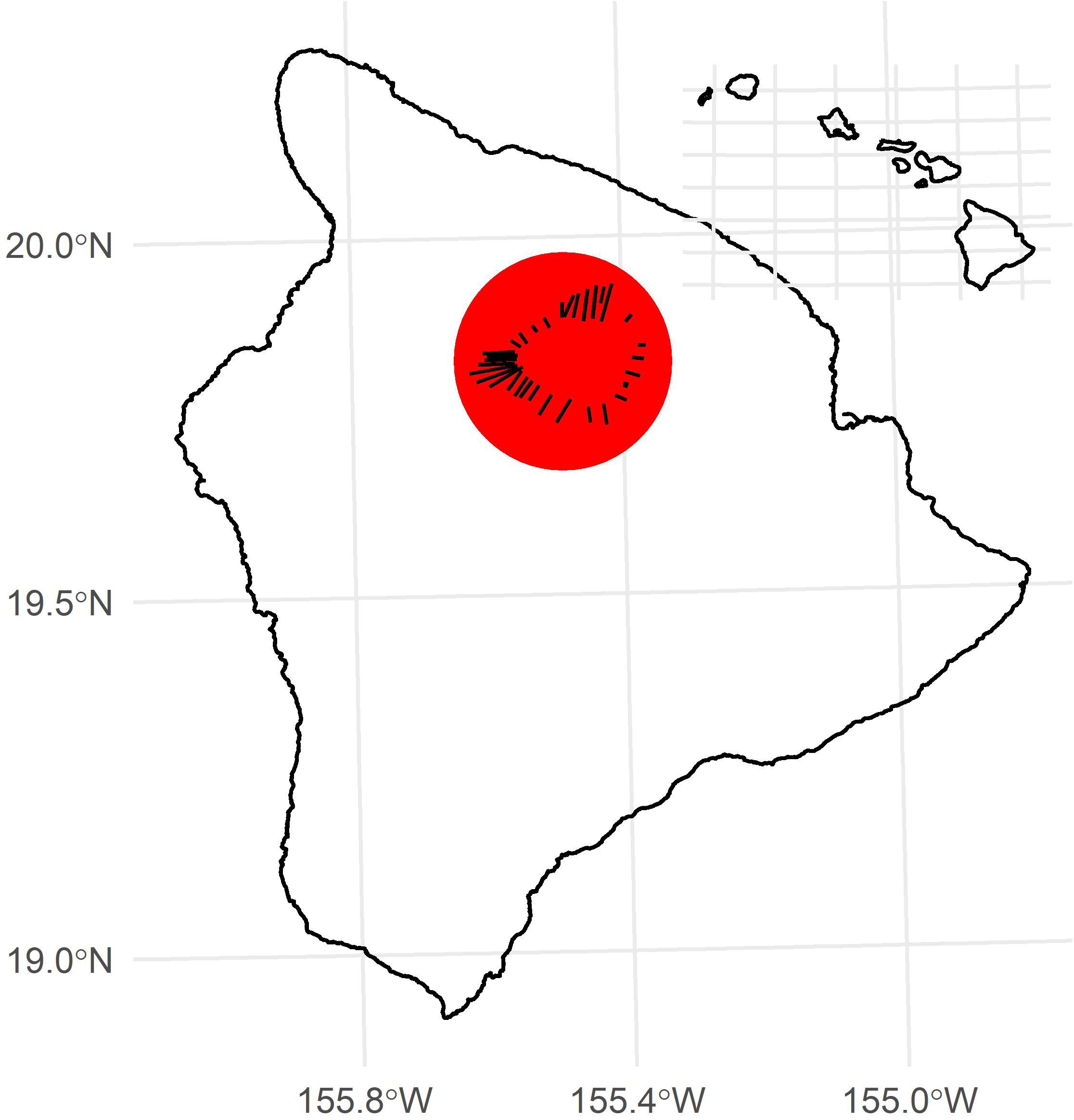
Figure 1. Location of palila sampling (red dot) conducted on Mauna Kea, Island of Hawai’i. Black lines are survey transects sampled between 2020 and 2024.

Survey data

Annual point-transect distance sampling surveys for palila and other forest birds were conducted in the forests around Mauna Kea, Island of Hawai’i starting in 1980 (Scott et al., 1984). The sampling frame was changed in 1998 when additional transects were added on the southwestern slope to produce a more precise population estimate and provide more complete coverage of a core survey area containing > 95% of palila detections (hereafter, core area; Johnson et al., 2006; Leonard et al., 2008). Since 2020, no palila have been detected outside the core area despite expanded sampling during annual surveys in 2022, 2023 and 2024 (Hunt et al., 2025). Within the core area, sampling points were spaced approximately 150 m apart on 13 transects between 3 km and 7.5 km in length that descended from the tree line. During a six-minute count at each point, trained observers recorded the species, detection type (heard, seen, or both), and distance of each bird from the observer. Time of sampling and weather conditions (cloud cover, rain intensity, wind strength, and gust strength) were also recorded, and surveying was postponed when conditions hindered the ability to detect birds (wind and gust strengths > 20 kph, e.g., Beaufort scale ≥ 4, or heavy rain). Counts commenced at sunrise and continued up to four hours. For our analyses, we evaluated patterns from annual point count data collected during the first quarter of 2020 through 2024 (hereafter annual surveys) and quarterly point count data collected from the second quarter of 2022 through the second quarter of 2024 (hereafter quarterly surveys; 12 surveys in total). The quarterly surveys were initially spatially restricted to the upper portions of transects where palila were detected during annual surveys, a subset of the annual survey sampling points. Starting in 2023, the spatial extent of the quarterly surveys was expanded to include the upper and middle portions of transects, an area that included the entire distribution of palila (Figure 2).

Figure 2

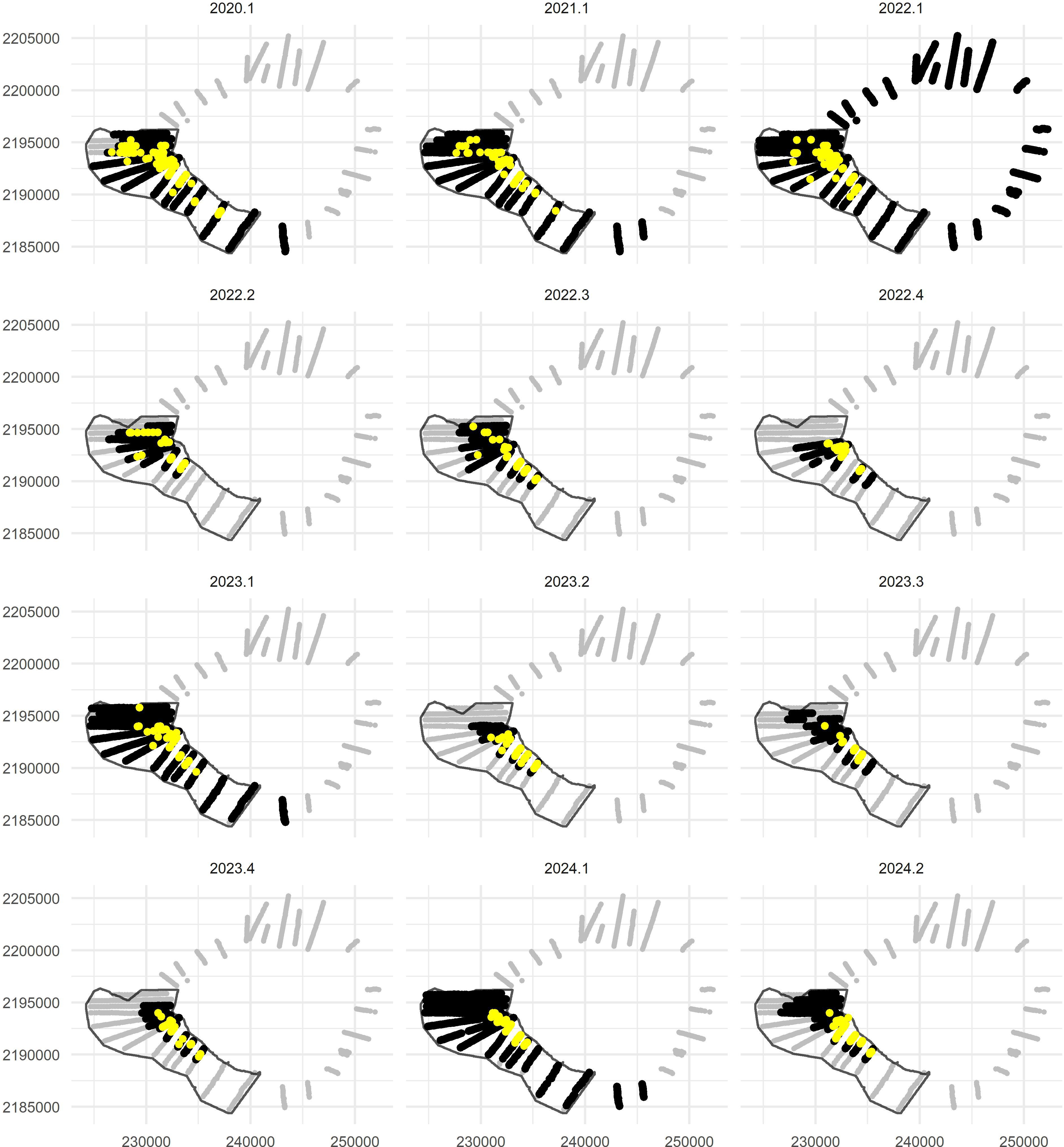
Figure 2. Location of samples and palila detections during each survey conducted on Mauna Kea, Island of Hawai’i, from 2020 through 2024 (refer to Figure 1 for study area location). Survey points are represented with gray dots, points sampled during a specific survey are represented with black dots, and points where one or more palila were detected are represented with yellow dots. The black polygon is the core study area. Base map from World Geodetic System 1984 (WGS84) zone 5 from U.S. Geological Survey’s National Elevation Dataset (USGS (U.S. Geological Survey), 2014).

Detection function modeling

Miller et al. (2013) describe a “2-stage” density modeling approach whereby the detection probability is modeled in the first stage using distance sampling methods and is then passed to and used as an offset term in a generalized additive model (GAM), which predicts counts based on smooth functions of spatial and temporal covariates. Using the Distance package (Miller et al., 2019) in R (R Core Team, 2024) we fitted half-normal and hazard-rate key detection functions and the key models with either adjustment terms or covariates to estimate the detection probability. Preliminary analysis revealed key detection functions with adjustment terms were not strictly monotonic, and there were only sufficient detections per factor to model the covariate survey (year and quarter). Data were truncated at a distance w where the estimated detection probability (using a preliminary detection function model) was about 0.1. Model selection for the detection function used Akaike information criterion (AIC) and model fit was evaluated with a Cramér-von Mises test (Buckland et al., 2015). Our approach follows methods detailed in Thomas et al. (2010) and Buckland et al. (2015). Data manipulation was performed using the tidyverse package (Wickham, 2022) and figures were generated using the ggplot2 package (Wickham et al., 2022) in the RStudio (RStudio Team, 2023) integrated development environment of program R.

The detection probability from distance sampling was entered in the smoother model as an estimated offset, which adjusts counts for undetected animals (Camp et al., 2020). In practice the detection probability variance, i.e., the variance in the slope of the probability density function of detected distances, is small (<< 10%) while the variation in counts among points, the encounter rate variance, typically dominates the component percentages of uncertainty in density estimates (Camp et al., 2009; Buckland et al., 2015). Thus, not propagating the detection probability variance through the GAM likely had minimal effect in underestimating total uncertainty while the encounter rate variability was efficiently modeled in a principled way via the smoother model (Camp, 2021).

Smoother modeling

A soap film smoother was used to account for the complex study boundaries, including a polygon with concave arcs (Wood et al., 2008). Soap film smoothers require defining a study area boundary that constrains predictions by the survey sampling domain and the extent of the spatial predictor variables. A boundary encompassing the points was delineated using R package splancs (Bivand et al., 2017). Camp et al. (2023) provides a detailed description of how the boundary accounting for habitat was delineated. The study area bounded domain contained 91,409, 30x30 m cells and an area of 8,226.81 ha. The extent of core area used herein differs from that of Genz et al. (2022; 6,440 ha) and Hunt et al. (2025). The main difference between the study areas is that our expanded area includes the critical habitat on the west slope. The number and location of knots (knots identify the dimension of the basis function controlling the amount of wiggliness) spread throughout the bounded domain was a priori defined as a set of knots on a regular 20 x 20 grid (400 total knots) using the make.soapgrid function of the dsm package (Miller et al., 2020). There were 138 knots inside the domain. The soap smoother is a two-component smooth where one component models the surface delineated by a domain and the other component models the polygon bounding the domain (i.e., the soap boundary). Density values on the boundary were fixed to zero as the breeding population of palila occurs only within the core area (Banko and Farmer, 2014).

The response variable, count, was a discrete, non-negative value and is reasonably modeled with Poisson, negative binomial, and Tweedie distributions. We checked model assumptions through inspection of the deviance residuals and refitting the selected model, with intercept, to the residuals to determine the amount of any remaining residual variance following methods described by Marra et al. (2012) and Wood (2017).

The models were built in R using the mgcv package (Wood, 2016). The mgcv optimization routine used to fit smooth terms is designed to balance the bias-variance trade-off (Wood, 2017) and we used restricted maximum likelihood (REML) methods to estimate smoothing parameters. We used AIC to select among the combination of smoother models following guidance provided in Wood (2017). We estimated abundances and their uncertainty using a Metropolis-Hastings sampler. A Metropolis-Hastings sampler is a simulation method for obtaining a random draw of samples from a posterior distribution, and the Metropolis-Hastings sampler is more appropriate both for counts that are not approximately Gaussian and for spatial models where large areas have zeros, which were common in the palila dataset. We obtained 1,000 replicate parameter value sets from the posterior distribution of densities based on a Metropolis-Hastings sampler with a vector of covariates conditional on the data and the posterior variance-covariance matrix. We used a burn-in of 10,000 samples and set the sampler with t-distribution degrees of freedom (t.df) of 15 and a random walk step (rw.scale) size of 0.04. A t.df controls the amount of sampling from the tails of the density distribution with a small value sampling more from the tails. The t.df value was increased from 15 by 5 until biologically unrealistic population estimates were excluded (> 8,000 individuals; the maximum 95% CI upper limit from Genz et al., 2022). We increased the size of the random walk step from 0.01 by hundredths until the acceptance probability was about a quarter (Wood, 2016). We refitted the linear predictor matrix to the replicate sets and estimated abundance as the mean and median of the replicate sets and SE as the standard deviation of the replicates. The 95% confidence intervals (CIs) were computed from the 2.5th and 97.5th quantiles.

Results

The number of points sampled varied from 116 to 212 for the quarterly surveys (quarters 2, 3 and 4) and from 444 to 742 for annual surveys (quarter 1; Figure 2). More than twice as many palila were detected during annual surveys (49—141; 84.6 ± 37.9 SD), which sampled all of the palila core survey area, than were detected during the second through fourth quarterly counts (14—65; 42.1 ± 17.1; Figure 2).

The hazard-rate detection function with covariate for survey (year and quarter) was > 28 AIC units smaller than other models (Supplementary Table S1). Key models including adjustment terms either failed to converge, were not monotonically decreasing, or were not selected. The Cramér-von Mises test for the best-fit model was non-significant at the alpha = 0.05 level indicating that the detection function provided a satisfactory fit to the distance histogram. Inspection of diagnostic plots also indicated that the model adequately fit the data (Supplementary Figure S1). Truncation distance was w = 87.5 m yielding 615 observations from 3,740 points. The effective area surveyed was $\widehat{\nu }$ = 1.352 ha and the detection probability was $\widehat{p}$ = 0.562 (SE = 0.028).

The Tweedie distribution had the lowest AIC by > 31 AIC units and inspection of residual quantile-quantile (QQ) plots showed that the Tweedie distribution gave the best fit to the data (Supplementary Table S2, Supplementary Figure S2). Inspection of the Tweedie distribution diagnostic plots fitted with a soap film smoother for spatial variables and a temporal smooth, the full model, revealed that the residual errors showed acceptable behavior (Supplementary Table S3, Supplementary Figure S3). The estimated Tweedie over-dispersion parameter was 1.101 and the scale parameter was 1.666 while the deviance explained was 47.4% for the full model (Supplementary Figure S4). The effective degrees of freedom values were approximately zero for the model refitted to the residuals, suggesting that there was little un-modeled residual structure (Supplementary Table S4).

Throughout the timeseries, there was a high-density palila hotspot in the east, central portion of the core area that is surveyed annually (Figure 3). Palila density remained low along the entire southern portion, lower southwestern boundary, and northern lobe of the core survey area. We defined the hotspot as cells with predicted densities > 0.5 birds/ha, a density that is relatively high for the rare palila and useful for management planning. The extent of the hotspot contracted 66% from 686 ha in the first quarter of 2020 to 231 ha in the second quarter of 2024, and the rate of range contraction was relatively constant across the timeseries (Supplementary Table S5). While the hotspot was contracting, the area extent of very low densities, < 0.25 birds/ha, in the 8,227-ha core area increased by only 7% from 7,203 ha in the first quarter of 2020 to 7,732 ha in quarter two of 2024.

Figure 3

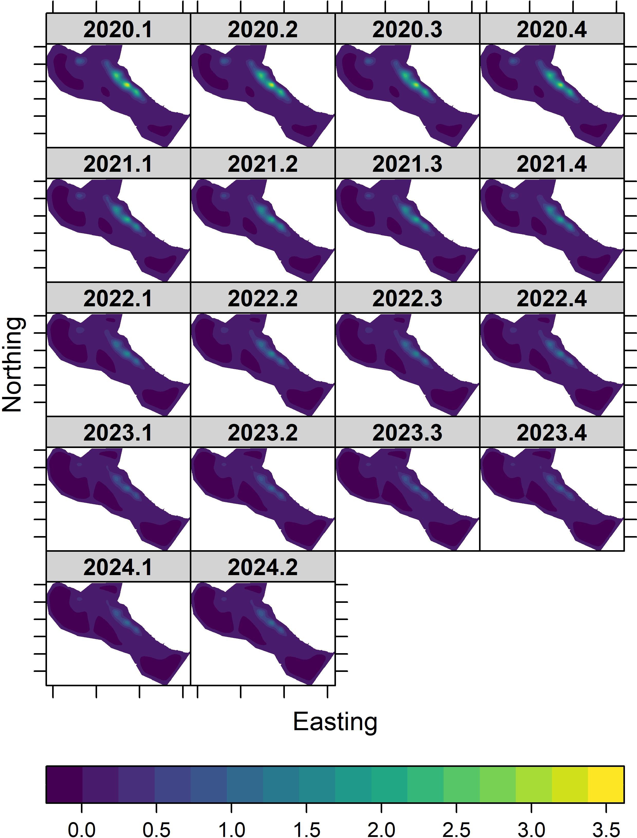
Figure 3. Predicted spatio-temporal surfaces of palila densities in the core survey area on Mauna Kea between 2020 and 2024. Densities range from 0 (violet) to 3.5 birds/ha (yellow).

Densities within the hotspot declined from about 3.4 birds/ha in 2020 to less than 1.2 birds/ha in each quarter in 2023 and 2024. The distribution of standard errors followed the same pattern seen in densities (Figure 4). Uncertainties were greatest in the east, central portion of the core survey area and were zero or near zero elsewhere in the core survey area. As the palila population declined throughout the timeseries, standard errors declined from a high of 1.7 birds/ha in 2020 to about 0.6 birds/ha in each quarter in 2023 and 2024. The spatial distribution of coefficients of variation remained consistent throughout the timeseries (Supplementary Figure S5), indicating that the spatial distribution and ratio in uncertainty in density and standard error estimates has changed little.

Figure 4

Figure 4. Predicted spatio-temporal surfaces of palila standard errors in the core survey area on Mauna Kea between 2020 and 2024. Standard errors range from 0 (violet) to 1.8 birds/ha (yellow).

Overall, we observed that the palila range had contracted (i.e., smaller extent of the hotspot) and densities within the contracting range had declined across the timeseries, which resulted in declining abundance from about 1,500 palila in 2020 (95% CI 1,264—1,949) to about 530 palila in the second quarter of 2024 (95% CI 421—669; Table 1). This decline was significant over the 5-year timeseries (F_1,10 = 90.4, p <0.001; Figure 5). Palila declined sharply between 2020 and 2023, but abundances since the first quarter of 2023 have fluctuated at 500 or fewer birds and abundances increased slightly during the first two quarters of 2024 to just over 500 birds.

Table 1

Table 1. Predicted palila abundance and uncertainty on Mauna Kea between the first quarter of 2020 and the second quarter of 2024.

Figure 5

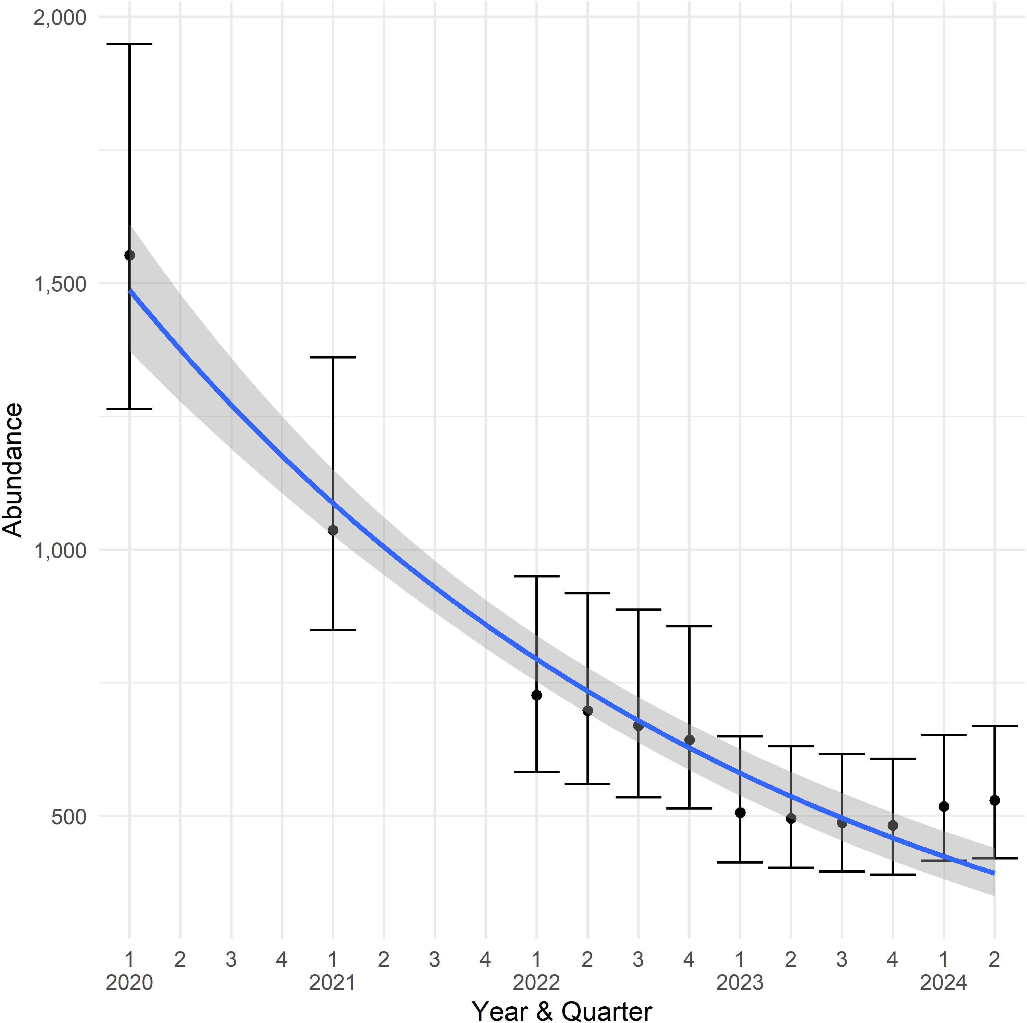
Figure 5. Palila population estimates from annual and quarterly surveys between 2020 and 2024 on the southwestern slope of Mauna Kea. The closed circles are the mean point estimate and whisker bars are the 95% confidence interval of the point estimates, the line represents the best fit log-linear regression, and the shaded area shows the 95% confidence interval of the trend.

Discussion

Understanding species’ distribution can help to inform effective species’ management and conservation. We fitted a generalized additive model with a soap film smoother and detectability, first estimated using conventional distance sampling, entered as an estimated offset, which adjusts counts for undetected animals, a DSM, to simultaneously identify the distribution and estimate the density of palila based on quarterly surveys. Our results indicate that palila maintained a high-density hotspot throughout the five-year timeseries, and that the hotspot was in the same location as that identified in 2017 (Camp et al., 2023). The extent of the hotspot with densities > 0.5 birds/ha, however, declined substantially over the timeseries from nearly 700 ha in 2020 to just over 200 ha in 2024, indicating a 66% range contraction. In 2017, the extent of the hotspot estimated using excursion set analysis with densities > 1 bird/ha was about 1,500 ha (Camp et al., 2023). The equivalent high-density area with palila > 1 bird/ha in the second quarter of 2024 was only 11 ha, or a 93% decline in the extent of the hotspot in just 7 years. Moreover, areas where palila were rare remained so throughout the timeseries and there was no indication that the location of the density hotspot had changed, either moving up- or down-slope or migrating east or west, among seasons. Management efforts, such as increased mammalian and avian predator control, predator exclusion, and supplemental feeding, that coincide with the location of the hotspot could therefore help arrest the decline of palila, although expanding management to enlarge the hotspot or to facilitate other hotspots may be needed to increase population persistence in the longer term.

Contraction of the palila hotspot was matched with declines in abundance. Densities within the hotspot declined from about 3 birds/ha in 2020 to about 1 bird/ha in 2024. The combined contracting hotspot and decreasing density yielded correspondingly lower abundances and a downward trend across the timeseries (Figure 5). We observed a 66% decline in abundance over 5 years, which was on par with the decline Genz et al. (2022) observed in the decade between 2012 and 2021 (54%), but substantially less than the 89% decline they observed for the 23-year period 1998 to 2021. The decline evident in the quarterly surveys since 2020 also corroborates the trend of declining annual abundances that Hunt et al. (2025) observed over the most recent 5- and 10-year trends from 2019 and 2014, respectively. Because of the different methods, our DSM estimates were some 240 to 330 birds higher than estimates by Genz et al. (2022) who used distance sampling (DS) methods. We used the same truncation distance (87.5 m) and hazard-rate key detection function as Genz et al. (2022) and Hunt et al. (2025); however, we incorporated additional survey data, fit a spatio-temporal-correlated smoother model instead of a standard distance sampling model, and estimated confidence intervals using a Metropolis-Hastings sampler instead of bootstrap procedures used in standard distance sampling analyses. Despite our abundances differing by roughly 148 birds less (in 2024) to 357 birds more (in 2021) than Hunt et al. (2025), the confidence intervals bracketed the mean point estimates in all but the 2021 survey, indicating that the differences were not statistically significant.

Uncertainty in the DSM estimates was relatively large (mean CV = 32.6%, standard deviation (SD) = 1.8) compared to uncertainty of the annual DS estimates by Genz et al. (2022; 2020 = 15.0% CV and 2021 = 18.7% CV) and Hunt et al. (2025; mean = 18.9%, SD =2.4). Similarly, Camp et al. (2023) observed that the DSM estimate was less precise than the DS estimate for palila in 2017. In contrast to comparing CVs, the confidence interval widths (CI widths) can be calculated following methods described in Camp et al. (2020) to compare the performance of DSM and DS methods. DSM gives on average a CI width that was 74.7% shorter than the CI widths using the DS methods of Hunt et al. (2025; SE = 26.8; Table 1). This pattern matches the shorter CI widths using DSM methods for Hawai’i ‘ākepa (Loxops coccineus), where Camp et al. (2020) observed that CI widths were 37% shorter using DSMs compared to DS methods. Our DSM method accounted for spatio-temporal correlation in palila counts that yielded substantial reduction in the length of the CI widths compared to DS methods. Moreover, quarterly surveys early in the time series were less structured and had slightly larger CVs than the more recent quarterly survey that followed a more standardized, formal structure with greater spatial coverage (CV = 0.32 vs. CV = 0.30; Table 1, Figure 2). The narrower CIs of DSMs increases the ability to detect population trends.

Quarterly surveys occurred predominately within the hotspot, an area where palila were known to occur based on previous annual surveys. This targeted sampling prohibited estimating abundance using standard distance sampling (Buckland et al., 2015); however, when combined with the more extensive annual surveys, the quarterly surveys may better inform palila distribution and density estimates when analyzed using GAMs within the DSM framework. Although palila are not territorial, they show strong site tenacity and their small home ranges are confined to the core area throughout the year (Fancy et al., 1993). Based on radio tracking data, palila median distances moved was relatively short and similar during both breeding and non-breeding seasons (349 ± 81 m and 388 ± 34 m, respectively). Thus, it is unlikely that birds moved or migrated outside of the hotspot during our time series; therefore, substantiating our spatially explicit extrapolation of the quarterly surveys. The extent of the sampling in earlier quarterly surveys was limited to short segments of transects within the palila hotspot and had slightly less precise estimates than the more recent quarterly surveys that were more standardized and had greater spatial coverage, sampling large sections of several transects across the palila hotspot. The quarterly surveys in 2023 had the least amount of spatial coverage and the largest CVs; thus, precision was positively related to the extent of spatial coverage of the surveys with greater coverage yielding greater precision. GAMs take advantage of the spatial association of the observations through modeling the spatial autocorrelation, assuming that observations close to each other are more likely to be similar (Legendre, 1993). GAMs are a semiparametric extension of generalized linear models (Hastie and Tibshirani, 1990) and have the advantages that the relationship between the natural processes response and explanatory variables are often better approximated using curvilinear models and that the data determines the shape of the response. Temporal and other explanatory variables, such as elevation, precipitation, and land cover type, can be included in GAMs, and we added a term to account for temporal autocorrelation in our model. Interpolation then yields predicted estimates for locations with no observations, which allows us to combine the quarterly surveys with the extensive annual surveys to produce maps of seasonal population distribution and density.

Our spatio-temporal GAM accounted for 47% of the deviance, and accounting for temporal autocorrelation explained 2% more deviance than the spatial-only GAM fitted to the 2017 survey (Camp et al., 2023). Thus, spatial autocorrelation remained (Supplementary Figure S4). Expanding the quarterly sampling by establishing more transects within and adjacent to the hotspot could improve model inference and sampling on a high-density grid would be expected to better capture the spatial correlation among sampling points compared to the current low-density, irregular spaced point sampling frame, which should yield more precise population estimates (Cressie and Wikle, 2011). Although switching to a high-density grid would not be needed to track changes in palila densities and may not yield substantial improvement in DS-based estimates, it would substantially increase survey effort. Passive acoustic monitoring using autonomous recording units may be an efficient alternative technique for surveying palila (Navine et al., 2024b). Moreover, Navine et al. (2024a) demonstrated that there is generally a strong correlation in call density estimated with Perch (Google Perch Bird vocalization Classifier; Denton et al., 2023, 2024) and bird densities estimated using distance sampling in Hawaiian forest birds.

Expanding the spatial coverage of the quarterly surveys to sample upslope and downslope and east and west of the hotspot could provide data on palila movement and resource use to inform effective conservation and management decision-making. Palila may be concentrating in the hot spot due to the small population and social preferences and interactions, and a lack of additional high quality māmane forest available elsewhere in the core-survey area. Historically, the māmane forest was heavily impacted by ungulates but regeneration of māmane and other native plants have improved following sheep (Ovis aries and O. a. musimon) and goat (Capra hircus) removals of the 1980s and 1990s (Hess et al., 1999; Banko et al., 2014). Ungulate control continues with aerial shooting and public hunting to maintain lower ungulate numbers (C. K. Asing, University of Hawai’i – Mānoa, written communication, 2024) and qualitatively there is less browse damage and more understory since earlier ungulate removals, thus, palila may no longer be limited by ungulate browse that previously limited the availability of māmane pods (Banko et al., 2014). Instead, palila may be limited by arthropod or other food resources, and expanded spatial coverage of the quarterly surveys may provide information on palila movement to other potential high-quality habitats. Mapping of the palila DSM overlayed with current management areas could lead to increased overall effectiveness. This would provide information necessary to identify areas for follow-up resource use research and target where additional management actions may be most beneficial to the species long-term survival.

Conclusions

A major goal of our study was to combine quarterly surveys with annual surveys within a DSM framework to identify and map seasonal changes in palila distribution and density. Our DSM incorporating spatial and temporal autocorrelation yielded annual abundance estimates similar to those of Genz et al. (2022) and Hunt et al. (2025), but our DSM estimates yielded substantially shorter CI widths, which improved our understanding of population trends, and our upper confidence limit can be used as the maximum population size to help guide management and conservation decisions. Based on quarterly surveys, the location of the palila high-density hotspot has not changed, but the size of the hotspot has contracted 66% to slightly more than 200 ha, and densities within the hotspot declined from about 3 birds/ha in 2020 to about 1 bird/ha in 2024. Palila may benefit most in the short-term if management actions were applied within the remaining hotspot. Further intervention is likely needed to halt range contraction, arrest population declines, and prevent their extinction. We conclude that our approach to include the spatially limited, quarterly surveys with the more extensive annual surveys produced accurate inferences for palila. Our modeling approach can be extended to other taxa and systems; however, caution is advised in applying our modeling approach for species that move much outside the extent of the most limited surveys.

Data availability statement

The raw data supporting the conclusions of this article will be made available by the authors, without undue reservation.

Ethics statement

The animal study was approved by University of Hawai’i Institutional Animal Care and Use Committee. The study was conducted in accordance with the local legislation and institutional requirements.

Author contributions

RC: Conceptualization, Formal analysis, Funding acquisition, Investigation, Methodology, Visualization, Writing – original draft, Writing – review & editing. CA: Data curation, Writing – review & editing. NH: Formal analysis, Writing – original draft, Writing – review & editing. AW: Data curation, Writing – review & editing. CF: Data curation, Writing – review & editing. LN: Funding acquisition, Writing – review & editing. PB: Conceptualization, Data curation, Writing – original draft, Writing – review & editing.

Funding

The author(s) declare that financial support was received for the research and/or publication of this article. Funding for surveys was provided by State of Hawaii, Department of Land and Natural Resources. Funding for analyses was provided by U.S. Geological Survey Ecosystems Mission Area to Richard Camp.

Acknowledgments

We thank the many trained bird counters who collected the data. We thank two reviewers for comments that improved our manuscript.

Conflict of interest

The authors declare that the research was conducted in the absence of any commercial or financial relationships that could be construed as a potential conflict of interest.

Generative AI statement

The author(s) declare that no Generative AI was used in the creation of this manuscript.

Publisher’s note

All claims expressed in this article are solely those of the authors and do not necessarily represent those of their affiliated organizations, or those of the publisher, the editors and the reviewers. Any product that may be evaluated in this article, or claim that may be made by its manufacturer, is not guaranteed or endorsed by the publisher.

Author disclaimer

Any use of trade, firm, or product names is for descriptive purposes only and does not imply endorsement by the U.S. Government.

Supplementary material

The Supplementary Material for this article can be found online at: https://www.frontiersin.org/articles/10.3389/fcosc.2025.1564661/full#supplementary-material

References

Bak T., Mullin S., Kohler E., Eichelberger B., and Camp R. J. (2024). Forest bird population trends on a small Oceanic Island. Global Ecol. Conserv. 56, e03273. doi: 10.1016/j.gecco.2024.e03273

Crossref Full Text | Google Scholar

Banko P. C. and Banko W. E. (2009). “Evolution and ecology of food exploitation,” in Conservation biology of Hawaiian forest birds: implications for island avifauna. Eds. Pratt T. K., Atkinson C. T., Banko P. C., Jacobi J. D., and Woodworth B. L. (Yale University Press, New Haven, Connecticut, USA), 159–193.

Google Scholar

Banko P. C., Brinck K. W., Farmer C., and Hess S. C. (2009). “Palila,” in Conservation biology of Hawaiian forest birds: implications for island avifauna. Eds. Pratt T. K., Atkinson C. T., Banko P. C., Jacobi J. D., and Woodworth B. L. (Yale University Press, New Haven, Connecticut, USA), 513–529.

Google Scholar

Banko P. C., Camp R. J., Farmer C., Brinck K. W., Leonard D. L., and Stephens R. M. (2013). Response of palila and other subalpine Hawaiian forest bird species to prolonged drought and habitat degradation by feral ungulates. Biol. Conserv. 157, 70–77. doi: 10.1016/j.biocon.2012.07.013

Crossref Full Text | Google Scholar

Banko P. C. and Farmer C. (Eds.) (2014). Palila restoration research 1996–2012. Hawai‘i Cooperative Studies Unit Technical Report HCSU-046 (Hilo, Hawaii: University of Hawai‘i). doi: 10790/2618

Google Scholar

Banko P. C., Hess S. C., Scowcroft P. G., Farmer C., Jacobi J. D., Stephens R. M., et al. (2014). Evaluating the long-term management of introduced ungulates to protect the palila, an endangered bird, and its critical habitat in subalpine forest on Mauna Kea, Hawaii. Arctic Antarctic Alpine Res. 46, 871–889. doi: 10.1657/1938-4246-46.4.871

Crossref Full Text | Google Scholar

Banko P. C., Johnson L., Lindsey G. D., Fancy S. G., Pratt T. K., Jacobi J. D., et al. (2020). “Palila (Loxioides bailleui), version 1.0,” in Birds of the World. Eds. Poole A. F. and Gill F. B. (Cornell Lab of Ornithology, Ithaca, NY, USA). doi: 10.2173/bow.palila.01

Crossref Full Text | Google Scholar

Banko P. C., Oboyski P. T., Slotterback J. W., Dougill S. J., Goltz D. M., Johnson L., et al. (2002). Availability of food resources, distribution of invasive species, and conservation of a Hawaiian bird along a gradient of elevation. J. Biogeography 29, 789–808. doi: 10.1046/j.1365-2699.2002.00724.x

Crossref Full Text | Google Scholar

BirdLife International (2021). Species factsheet: Loxioides bailleui. Available online at: http://www.birdlife.org (Accessed October 21, 2024).

Google Scholar

Bivand R., Rowlingson B., Diggle P., Petris G., and Eglen S. (2017). Splancs: spatial and space-time point pattern analysis. R package version 2.01-40. Available at: https://CRAN.R-project.org/package=splancs.

Google Scholar

Buckland S. T., Rexstad E. A., Marques T. A., and Oedekoven C. S. (2015). Distance sampling: methods and applications (London, UK: Springer).

Google Scholar

Burney D. A., James H. F., Burney L. P., Olson S. L., Kikuchi W., Wagner W. L., et al. (2001). Fossil evidence for a diverse biota from Kaua‘i and its transformation since human arrival. Ecol. Monogr. 71, 615–641. doi: 10.1890/0012-9615(2001)071[0615:FEFADB]2.0.CO;2

Crossref Full Text | Google Scholar

Camp R. J. (2021). Improved methods for estimating spatial and temporal trends from point transect survey data. University of St Andrews, St Andrews (UK.

Google Scholar

Camp R. J., Asing C. K., Banko P. C., Berry L., Brinck K. W., Farmer C., et al. (2023). Density surface and excursion sets modeling as an approach to estimate population densities. J. Wildlife Manage. 87, e22332. doi: 10.1002/jwmg.22332

Crossref Full Text | Google Scholar

Camp R. J., Miller D. L., Thomas L., Buckland S. T., and Kendall S. J. (2020). Using density surface models to estimate spatio-temporal changes in population densities and trend. Ecography 43, 1079–1089. doi: 10.1111/ecog.04859

Crossref Full Text | Google Scholar

Camp R. J., Reynolds M. H., Woodworth B. L., Gorresen P. M., and Pratt T. K. (2009). “Monitoring Hawaiian forest birds,” in Conservation Biology of Hawaiian Forest Birds: Implications for insular avifauna. Eds. Pratt T. K., Atkinson C. T., Banko P. C., Jacobi J. D., and Woodworth B. L. (Yale University Press, New Haven, CT, USA), 83–107.

Google Scholar

Cressie N. and Wikle C. K. (2011). Statistics for spatio-temporal data (New York, New York, USA: John Wiley & Sons).

Google Scholar

Denton T., Dumoulin V., Hamer J., Triantafillou E., and van Merriënboer B. (2023). Perch Google Bird Vocalization Classifier. Available online at: https://www.kaggle.com/models/google/bird-vocalization-classifier (Accessed December 14, 2024).

Google Scholar

Denton T., Dumoulin V., Triantafillou E., Hamer J., Schulist M., Morris D., et al. (2024). Perch. Available online at: https://github.com/google-research/perch (Accessed December 14, 2024).

Google Scholar

Fancy S. G., Sugihara R. T., Jeffrey J. J., and Jacobi J. D. (1993). Site tenacity of the endangered palila. Wilson Bull. 105, 587–596.

Google Scholar

Genz A. S., Brinck K. W., Asing C. K., Berry L., Camp R. J., and Banko P. C. (2022). 2019–2021 palila abundance estimates and trend. Hawaii Cooperative Studies Unit Technical Report HCSU-101 (Hilo, Hawaii: University of Hawaii at Hilo).

Google Scholar

Giambelluca T. W., Chen Q., Frazier A. G., Price J. P., Chen Y., Chu P., et al. (2013). Online rainfall atlas of Hawai‘i. Bull. Am. Meteorological Soc. 94, 313–316. doi: 10.1175/BAMS-D-11-00228.1

Crossref Full Text | Google Scholar

Gorresen P. M., Camp R. J., Reynolds M. H., Woodworth B. L., and Pratt T. K. (2009). “Status and trends of native Hawaiian songbirds,” in Conservation Biology of Hawaiian Forest Birds: Implications for insular avifauna. Eds. Pratt T. K., Atkinson C. T., Banko P. C., Jacobi J. D., and Woodworth B. L. (Yale University Press, New Haven, CT, USA), 108–136.

Google Scholar

Hastie T. and Tibshirani R. (1990). Generalized additive models, monographs on statistics and applied probability, vol 43 (New York, USA: Chapman and Hall).

Google Scholar

Hawaii Administrative Rules. (2013). List of species of endangered wildlife in Hawaii. Available at: https://dlnr.hawaii.gov/dofaw/files/2013/09/Chap124a-Ex.pdf (Accessed September 13, 2022).

Google Scholar

Hess S. C., Banko P. C., Brenner G. J., and Jacobi J. D. (1999). Factors related to the recovery of subalpine woodland on Mauna Kea, Hawaii. Biotropica 31, 212–219. doi: 10.1111/j.1744-7429.1999.tb00133.x

Crossref Full Text | Google Scholar

Hess S. C., Banko P. C., Miller L. J., and Laniawe L. P. (2014). Habitat and food preferences of the endangered palila (Loxioides bailleui) on Mauna Kea, Hawaii. Wilson J. Ornithology 126, 728–738. doi: 10.1676/13-220.1

Crossref Full Text | Google Scholar

Hess S. G., Banko P. C., Reynolds M. H., Brenner G. J., Laniawe L. P., and Jacobi J. D. (2001). Drepanidine movements in relation to food availability in subalpine woodlands on Mauna Kea, Hawaii. Stud. Avian Biol. 22, 154–163. Available online at: https://sora.unm.edu/sites/default/files/SAB_022_2001%20P154-163_Drepanidine%20Movements%20in%20Relation%20to%20Food%20Availabilty%20in%20Subalpine%20Woodland%20on%20Mauna%20Kea%20Hawaii_Hess,%20Banko,%20Reynolds,%20Brenner,%20Laniawe,%20Jacobi.pdf (Accessed December 14, 2024).

Google Scholar

Hunt N. J., Asing C. K., Neitmann L., Banko P. C., and Camp R. J. (2025). 2022–2024 Status and Trend of the Palila (Loxioides bailleui). Hawaii Cooperative Studies Unit Technical Report HCSU-115 (Hilo, Hawaii: University of Hawaii at Hilo).

Google Scholar

Johnson L., Camp R. J., Brinck K. W., and Banko P. C. (2006). Long-term population monitoring: lessons learned from an endangered passerine in Hawaii. Wildlife Soc. Bull. 34, 1055–1063. doi: 10.2193/0091-7648(2006)34[1055:LPMLLF]2.0.CO;2

Crossref Full Text | Google Scholar

LeBaron J. (2023). The 123^rd Christmas bird count summary: December 14, 2022 to January 5, 2023. Available online at: https://www.audubon.org/news/123rd-christmas-bird-count-summary (Accessed September 27, 2024).

Google Scholar

Legendre P. (1993). Spatial autocorrelation: trouble or new paradigm? Ecology 74, 1659–1673. doi: 10.2307/1939924

Crossref Full Text | Google Scholar

Leonard D. L. Jr., Banko P. C., Brinck K. W., Farmer C., and Camp R. J. (2008). Recent surveys indicate rapid decline of palila population. ‘Elepaio 68, 27–30. Available online at: https://hiaudubon.org/wp-content/uploads/2021/12/Elepaio68.4.pdf (Accessed December 14, 2024).

Google Scholar

Lindsey G. D., Fancy S. G., Reynolds M. H., Pratt T. K., Wilson K. A., Banko P. C., et al. (1995). Population structure and survival of palila. Condor 97, 528–535. doi: 10.2307/1369038

Crossref Full Text | Google Scholar

Link W. A. and Sauer J. R. (1998). Estimating population change from count data: application to the North American breeding bird survey. Ecol. Appl. 8, 258–268. doi: 10.1890/1051-0761(1998)008[0258:EPCFCD]2.0.CO;2

Crossref Full Text | Google Scholar

Marra G., Miller D. L., and Zanin L. (2012). Modelling the spatiotemporal distribution of the incidence of resident foreign population. Statistica Neerlandica 66, 133–160. doi: 10.1111/j.1467-9574.2011.00500.x.

Crossref Full Text | Google Scholar

Miller D. L., Burt M. L., Rexstad E. A., and Thomas L. (2013). Spatial models for distance sampling data: recent developments and future directions. Methods Ecol. Evol. 4, 1001–1010. doi: 10.1111/2041-210X.12105

Crossref Full Text | Google Scholar

Miller D. L., Rexstad E. A., Burt L., Bravington M. V., and Hedley S. (2020). dsm: Density surface modelling of distance sampling data. R package version 2.3.0. Available online at: https://github.com/DistanceDevelopment/dsm (Accessed April 25, 2024).

Google Scholar

Miller D. L., Rexstad E. A., Thomas L., Marshall L., and Laake J. L. (2019). Distance sampling in R. J. Stat. Software 89, 1–28. doi: 10.18637/jss.v089.i01

Crossref Full Text | Google Scholar

Navine A. K., Camp R. J., Weldy M. J., Denton T., and Hart P. J. (2024a). Counting the chorus: A bioacoustics indicator of population density. Ecol. Indic. 169, 112930. doi: 10.1016/j.ecolind.2024.112930

Crossref Full Text | Google Scholar

Navine A. K., Denton T., Weldy M. J., and Hart P. J. (2024b). All thresholds barred: Direct estimation of call density in bioacoustic data. Front. Bird Sci. 3. doi: 10.3389/fbirs.2024.1380636

Crossref Full Text | Google Scholar

Olson S. L. and James H. F. (1982). Prodromus of the fossil avifauna of the Hawaiian Islands. Smithsonian Contributions to Zoology 365, 1–59. doi: 10.5479/si.00810282.365

Crossref Full Text | Google Scholar

R Core Team (2024). R: a Language and Environment for Statistical Computing. Version 4.4.0 (Vienna, Austria: R Foundation for Statistical Computing). Available at: https://www.R-project.org (Accessed April 25, 2024).

Google Scholar

Richardson R. M., Amundson C. L., Johnson J. A., Romano M. D., Taylor A. R., Fleming M. D., et al. (2024). Rapid population decline in McKay’s Bunting, an Alaskan endemic, highlights the species’ current status relative to international standards for vulnerable species. Ornithological Appl. 126, duad064. doi: 10.1093/ornithapp/duad064

Crossref Full Text | Google Scholar

RStudio Team (2023). RStudio: Integrated development for R RStudio (Boston, Massachusetts, USA: PBC). Available at: https://posit.co/products/open-source/rstudio/.

Google Scholar

Scott J. M., Mountainspring S., van Riper C. III, Kepler C. B., Jacobi J. D., Burr T. A., et al. (1984). Annual variation in the distribution, abundance, and habitat response of the palila (Loxioides bailleui). Auk 101, 647–664. doi: 10.2307/4086892

Crossref Full Text | Google Scholar

Thomas L., Buckland S. T., Rexstad E. A., Laake J. L., Strindberg S., Hedley S. L., et al. (2010). Distance software: Design and analysis of distance sampling surveys for estimating population size. J. Appl. Ecol. 47, 5–14. doi: 10.1111/j.1365-2664.2009.01737.x

PubMed Abstract | Crossref Full Text | Google Scholar

USFWS (U.S. Fish and Wildlife Service) (1967). Endangered species list – 1967. Federal Registry 32 FR 4001. Available online at: https://archives.federalregister.gov/issue_slice/1967/3/11/4000-4002.pdf#page=2 (Accessed December 14, 2024).

Google Scholar

USGS (U.S. Geological Survey) (2014). National elevation dataset (NED): U.S. Geological Survey database. Available online at: http://nationalmap.gov/elevation.html.368 (Accessed December 14, 2024).

Google Scholar

van Riper C. III, Scott J. M., and Woodside D. M. (1978). Distribution and abundance patterns of the Palila on Mauna Kea, Hawaii. Auk 95, 518–527. doi: 10.1093/auk/95.3.518

Crossref Full Text | Google Scholar

Wickham H. (2022). Tidyverse: Easily install and load the ‘Tidyverse’, version 1.3.2. Available online at: https://1263tidyverse.tidyverse.org (Accessed February 22, 2023).

Google Scholar

Wickham H., Chang W., Henry L., Pedersen T. L., Takahashi K., Wilke C., et al. (2022). ggplot2: Create elegant data visualisations using the grammar of graphics. Version 3.4.0. Available online at: https://cran.r-project.org/web/packages/ggplot2/index.html (Accessed April 23, 2024).

Google Scholar

Wood S. N. (2016). mgcv: Mixed GAM computation vehicle with automatic smoothness estimation. R package version 1. (The Comprehensive R Archive Network (CRAN)). 8–28.

Google Scholar

Wood S. N. (2017). Generalized additive models: an introduction with R (Boca Raton, Florida, USA: CRC Press).

Google Scholar

Wood S. N., Bravington M. V., and Hedley S. L. (2008). Soap film smoothing. J. R. Stat. Society: Ser. B (Statistical Methods) 70, 931–955. doi: 10.1111/j.1467-9868.2008.00665.x

Crossref Full Text | Google Scholar