 Mark Witteveen
 Tiziano Natali
 Theo J. M. Ruers1,2
 Behdad Dashtbozorg
- 1Image-guided Surgery, Surgical Department, Netherlands Cancer Institute - Antoni van Leeuwenhoek, Amsterdam, Netherlands
- 2Department of Nanobiophysics, University of Twente, Enschede, Netherlands
Introduction: Optical property retrieval in diffuse reflectance imaging, like diffuse reflectance spectroscopy (DRS) and hyperspectral imaging (HSI), often involves fitting measured spectra to analytical solutions using approximations such as Diffusion Theory (DT). This method, while accurate, is not always generalizable due to the assumptions inherent in DT and results in non-unique solutions for optical properties and physiological parameters. In addition, it is computationally intensive. Physics-inspired deep learning offers generalizable data descriptions guided by physical principles but requires extensive labelled data, which is hard to obtain, especially in medical contexts.
Methods: We propose a deep learning approach to retrieve physiological parameters from DRS and HSI spectra using DT-simulated training data. The DT-simulated data is synthesised using a range for the optical properties: Blood Volume Fraction (BVF), Saturation, water-fat ratio (WFR), average blood vessel radius (R), scattering amplitude (SA), and scattering slope (SL). The range for these parameters we have extracted from literature.
Results: Our feed-forward neural network achieved median relative errors of 4% and 2% for DRS and HSI, respectively.
Discussion: Results suggest that the proposed method is robust and that retrieval of optical properties is possible with similar results to DT but also reducing operation time.
1 Introduction
Diffuse reflectance can be captured by various techniques such as Diffuse Reflectance Spectroscopy (DRS), where the acquisition is a point measurement using a fibre; and Hyperspectral Imaging (HSI), where the acquisition is a wide field measurement using a camera. DRS and HSI both utilize absorption and scattering differences of diffusely scattered light in tissue for categorization and discrimination of various tissue types, for example, in medical applications (Baltussen et al., 2017; Nogueira et al., 2021; Currà et al., 2019; De Boer et al., 2018; Baltussen et al., 2019; Pertzborn et al., 2024). Tissue classification/discrimination algorithms might be categorized into optical property-based and machine-learning-based approaches (Lu and Fei, 2014). Optical property-based techniques aim to retrieve tissue optical properties for tissue type discrimination (Witteveen et al., 2022a; Claridge and Hidovic-Rowe, 2014; Post et al., 2017). Retrieval is often performed through analytical descriptions of light propagation, such as the model presented by Farrell et al. (1992) for DRS or more complex or specific Monte Carlo Methods (Wang et al., 2005). They can accommodate complex tissue geometries and heterogeneous optical properties, providing detailed insights into light-tissue interactions. However, their computational intensity often necessitates the use of inverse Monte Carlo methods or hybrid approaches to retrieve optical properties efficiently.
A common method for optical property retrieval is achieved by using a description of the reflectance of tissue and applying an inverse fit to estimate absorption and scattering from captured spectra. Reduced scattering
where
The absorption can then be described as a combination of known chromophores at certain concentrations. For a general tissue, the following approximation of the absorption is used:
where the concentrations are denoted using
The physiological parameters used are: blood volume fraction (BVF), blood saturation (SAT), average radius of blood vessels (R), and water-fat ratio (WFR). Values for these physiological parameters are taken from Jacques (2013). Jacques (2013) With the parameters presented in (1) and (2), the absorption and reduced scattering for different tissue types can then be calculated. A model is used to calculate the diffuse reflection; taking the geometry into account for DRS; or as a wide-field approximation for HSI. A minimization technique (e.g., non-linear least squares) can be used to minimize the error between the measured and calculated spectra. The advantage of this approach is that all the acquired data is compared using a known and well-understood combination of parameters such as blood volume fraction, saturation, fat concentration, and reduced scattering parameters (de Boer et al., 2015; Adank et al., 2018; Witteveen et al., 2022a). However, minimization of the spectra is an iterative fitting process and thus often slow; it is also constrained by the model used and thus limited to the assumptions underlying the model. When noise, variation and unknowns are introduced in the spectra, the model might produce non-unique solutions (optical properties) for the same spectra. Therefore, alternative approaches could be implemented for both hyperspectral imaging and diffuse reflectance spectroscopy that are not constrained to the same degree.
In recent years, machine learning (ML) and deep learning (DL) techniques have been increasingly applied in biophotonics and spectroscopic applications for tissue discrimination (Pertzborn et al., 2024; Cui et al., 2022; Scarbrough et al., 2024; Fernandes et al., 2021). Unlike analytical approaches, deep learning (DL) methods rely on an algorithm’s ability to generalize from a dataset to predict unseen data. For instance, Livecchi et al. (2024) developed a DL approach to rapidly process hyperspectral image data and accurately quantify tissue components. Similarly, Brouwer de Koning and Ruers (2021) utilized DL semantic segmentation for tumor detection in hyperspectral images. A comprehensive review by ? discusses the integration of DL with hyperspectral imaging for disease diagnosis. These methods that utilize DL do not require rigid assumptions for retrieving optical properties that are intrinsic in conventional methods. However, due to scarcity of labels in measured data, deep-learning methods can be affected by over-fitting on smaller datasets, a phenomenon where the network focuses its learning on irrelevant spectral features that are only specific to the training set, resulting in failure to generalize correctly on unseen data (Power et al., 2022). While the generalizability of DL techniques may suffice for intra-study or intra-device comparisons, it may not extend well to inter-study or inter-device scenarios.
To overcome the limitations of conventional techniques in identifying a unique solution and to address over-fitting challenges in deep learning methods, a hybrid approach that combines physical modelling of light transport with deep learning could be employed. This approach would leverage the self-learning ability of DL techniques with the verifiable and easily interpretable values of physiological parameters of tissue, resulting in a more verifiable and explainable use of DL. Such a combination would additionally help with the discrimination and classification of clinical data. Finally, this approach would exploit the ability of DL to learn patterns in data while being easier to verify, check, and convey to clinical practice.
A major challenge in training deep learning (DL) models for optical property retrieval lies in the lack of clinically measured spectra with ground-truth physiological parameters. To address this, we propose training and evaluating DL models using simulated spectra, which enable controlled generation of data across a wide physiological parameter space. Simulated datasets have been successfully used in prior work—for example, in retrieving absorption and scattering coefficients from phantoms (Scarbrough et al., 2024) and thin tissue layers (Barberio et al., 2021). These studies demonstrate that synthetic data can serve as an effective training substitute when real labelled data is scarce; given that the parameter range is similar. Our approach introduces two key innovations. First, we use a simple feedforward neural network that applies single-normal variate (SNV) normalization to the optical parameters, improving consistency across samples. Second, we design a unified network architecture capable of processing data from both hyperspectral imaging (HSI) and point-based diffuse reflectance spectroscopy (DRS). This contrasts with prior work such as Livecchi et al. (2024), who trained separate artificial neural networks (ANNs) for different tissue models, which while accurate is increasingly complicated. By using a shared model for both imaging and probe-based spectra, we aim to reduce complexity and promote cross-modality generalization.
Since the approach is taken to train on synthetic data, a central focus of our method is robustness. We explicitly test the model not only on data sampled from within the original training range, but also on spectra generated from physiological parameters outside that range. This out-of-range evaluation is critical for assessing the model’s ability to generalize under unseen conditions. Our approach aligns with principles proposed by Hokr and Bixler (2021), who emphasized the importance of covering the full biologically relevant optical parameter space, and it extends these ideas by directly testing beyond typical bounds.
This robustness-focused approach complements recent developments in the field. For instance, Livecchi et al. (2024) developed a DL model to rapidly process hyperspectral images and quantify tissue components, while Scarbrough et al. (2024) introduced a wavelength-independent regressor that achieved low errors (1.5%–1.8%) on simulated data even under substantial spectral perturbations. Similarly, Hokr and Bixler (2021) trained their model to span several decades of optical properties by using statistical moments rather than spectral inputs. Our method builds upon these works by emphasizing simplicity, cross-modality design, and direct out-of-range validation.
In summary, this work makes the following key contributions:
2 Methods
The method proposed consists of two phases: data synthesis, using diffusion theory; and retrieval, using a deep learning network. The introduced pipeline is shown in Figure 1.
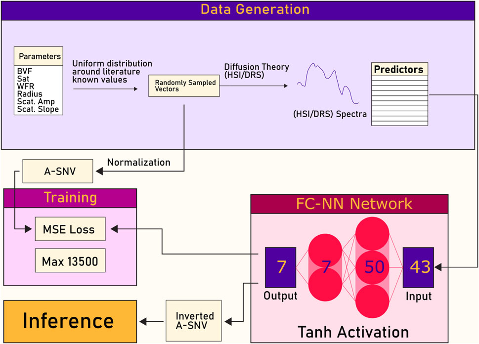
Figure 1. A simplified structure of the principle pipeline for the retrieval of optical properties using deep learning. Parameters are defined for synthetic generation of the spectra, which are used as the ground truth for the retrieved optical properties for the network. The network consists of a feed forward neural network (FF-NN), where the input is the spectra generated by diffusion theory and the output are the retrieved optical properties. Note that normalization is used due to the magnitude differences in the optical properties.
2.1 Synthetic data generation
For the generation of synthetic data using diffusion theory, the model of ? is used for the DRS spectra, and the model of Flock et al. (1989) is used for the HSI spectra. The wavelength range chosen is between 450 and 1,450 nm in 25 nm steps, covering the visual to SWIR range. These models are valid when absorption is much smaller than reduced scattering
Alternative models commonly used in DRS and HSI applications include the semi-empirical approach by Yudovsky and Pilon (2009), the two-point source diffusion approximation described by Jacques (1999), and models compared in recent evaluations such as Bahl et al. (2023). These models are known to more closely replicate reflectance from layered or semi-infinite tissues and improve agreement with both Monte Carlo simulations and phantom measurements. While the current models serve to illustrate the technique, future work will incorporate these alternatives to increase physiological relevance and model robustness.
The equations for the diffuse reflection in DRS are given by:
with:
where the parameters
where
where
The ranges of the optical properties, therefore also the six optical properties that are under investigation are shown in the table Table 1.
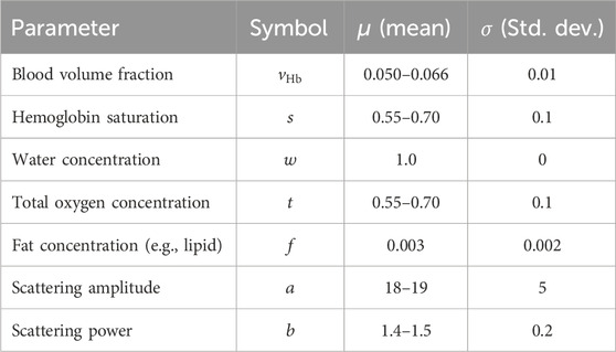
Table 1. Mean
To better approximate the expected measurements noise is added to the measurements. An empirically measured and modelled wavelength-dependent noise is added to the spectra generated by Equations 3, 6, this generates more realistic data than wavelength-independent noise, with the noise approximated by:
where
Several studies support this type of signal dependent and wavelength dependent noise modelling as a realistic approximation: Meola et al. (2011) provide a practical framework for hyperspectral noise estimation that accounts for amplitude dependence and spectral variability Meola et al. (2011) and Mahmood and Sears. (2021) extend this to estimate correlated signal-dependent noise statistics in HSI data Mahmood and Sears (2021). These findings are similar to our rationale that empirical wavelength-dependent noise models can closely emulate real sensor behaviour.
While these models improve simulation fidelity, future work should investigate how varying the coefficients in Equation 7, for example, changing an additional scaling factor, affects model performance and robustness in both network and diffusion theory outputs.
A uniform distribution function was used to vary the optical parameters for the diffusion model, presented in (6), where the optical parameters were within values expected in clinically measured tissue. The selection of the variables was performed using a uniform distribution created using a mean
The values used are shown in table Table 1.
2.2 Deep learning architecture
The architecture chosen for the DL network (Figure 1) was based on a multi-output feed-forward network, as commonly used for simple regression tasks Shi et al. (2009).
The network consists of 2 fully connected layers. The inputs for the network are the 1D spectra as obtained from the synthetic diffusion theory spectra, as described in section subsection 2.1. The output of the network consists of a list of optical properties, which can then be compared to the optical properties used to simulate the spectra. The network was implemented in Matlab 2022a (MathWorks Inc., Natick, Massachusetts, United States) using the ‘fitnet’ function. A maximum of 13,500 epochs was chosen, with an early stopping of 6 continuous epochs of increasing validation performance, which is necessary for preventing over-fitting of the model on the training dataset. A more detailed overview of the DL setup and the hyper-parameters used are show in Table 2. Furthermore, pseudocode for the fitting and evaluation of the data is presented in pseudocode Algorithm 1.
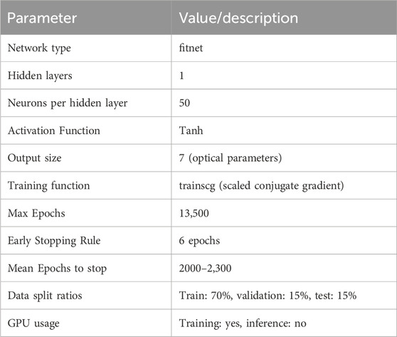
Table 2. Overview of parameters and constants used for training the neural network model.
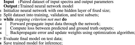
Algorithm 1. Supervised neural network training pipeline.
This architecture was chosen based on the nature of the data: each input spectrum is a fixed-length 1D vector without spatial structure or temporal dependencies, making it well-suited for a standard feed-forward neural network. The feed-forward network is a simple network, thus easier to reproduce and more suitable for this exploratory work. More complex architectures such as CNNs, RNNs, or Transformer-based models were not considered necessary, as they are designed to exploit spatial information, sequence modelling, or attention mechanisms, respectively. 2D-CNN or 3D-CNN could be used in the case of HSI where we have complicated spatial-spectral information, but for this application where each spectra is considered independently, feed forward networks are preferred. In this case, the problem can be effectively approached as a straightforward regression task, for which feed-forward networks have proven sufficient and efficient.
2.3 Diffusion theory fitting
To fit the diffusion theory, as described above, a non-linear least squares approach was used. The equation that is to be minimized is given by;
where
The non-linear least squares approach, as shown in Equation 8, is implemented in Matlab using a trust-region reflect algorithm, with a maximum of 1,500 iterations and being function evaluation limited to maximize accuracy of the resulting fit (Coleman and Li, 1996). Note that for every fitting procedure, a random initial starting value for every parameter is chosen to avoid biasing the result.
2.4 Extrapolation performance of network
To evaluate the network’s ability to estimate optical properties accurately outside its training range, two datasets are created. The first dataset includes optical properties that fall within the training range, serving as a baseline. The second dataset contains values outside the training range and is divided into six subsets. In each subset, one of the six optical properties is varied beyond the original range, while the remaining parameters stay within the training range. This design allows for a detailed assessment of the network’s generalizability and helps to identify the effect of unexpected input data on each of the six variables individually.
To increase the performance of the network and faster convergence, the optical properties given to the network were standardized using an adaptation of the SNV, which is given by the equation:
where
To measure the error between the estimated and actual values for the optical properties, the relative error (RE) is calculated for all the optical properties. The RE is calculated as:
where
As mentioned in subsection 2.1, a uniform distribution was chosen, instead of the clinically expected normal distribution, in order to ensure better generalizability of the DL model. If presented with a normal distribution, the network is more likely to overfit to the mean of the normal distribution, reducing the robustness of the network for values further away from the mean. The equation used for the uniform distribution is given by:
In this equation, the probability function of a uniform distribution is defined within the interval
To further verify the performance of the network a statistical test is done between the estimated values and the relative errors between diffusion theory and the network. A Wilcoxon rank sum test was performed with a Bonferroni correction and a significance level of 0.01.
3 Results
The results of the estimated optical properties are shown in Figures 2a,b. Here it can be seen that the estimated properties match the expected values for both diffusion theory fitting and for the network, with the absolute difference being between the highest for the scattering amplitude (SA) with a median difference to the ground truth of (DRS:-0.0065
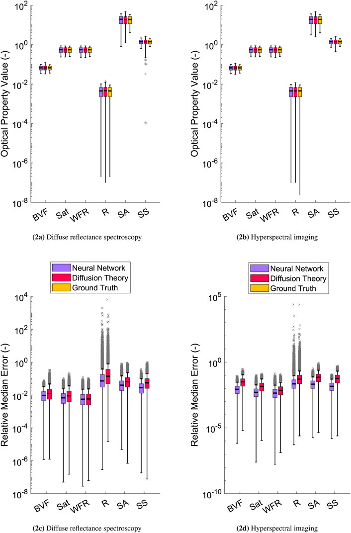
Figure 2. Value of the optical parameters for: (a,b) the ground truth (yellow), the diffusion theory estimated values (pink); and the network estimated values (purple), where the results are compared between the two approaches of inverse calculating. The relative error for DRS (c) and HSI (d) for the network (purple) and diffusion theory (pink). Outliers are shown with yellow crosses. Note that the error is relative, therefore more outliers are found in higher values than in lower values. With: blood volume fraction (BVF), blood saturation (SAT), average radius of blood vessels (R), water-fat ratio (WFR), scattering amplitude (SA), and scattering slope (SS).
Furthermore, the median relative error for the two models are shown in Table 3; as well as the speed of the calculation for the proposed network and DT. The DT approach is implemented using Matlab 2022a (MathWorks Inc., Natick, Massachusetts, United States), using multiple CPU cores to speed up the calculation. The network was implemented using Matlab running the CPU using the built-in method for evaluation. The difference in speed, from 2,486 s for diffusion theory to 0.097 s using the network, is shown in Table 3.
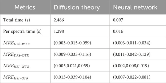
Table 3. The processing time the diffusion theory and the neural network approaches. The “Total time” metric is the total time for processing the entire test set, while the “Per spectra time” is exclusively the processing of a single spectrum.
In terms of accuracy, the neural network achieves comparable or improved performance across all modalities. For DRS data within the training range (WTR), the network achieves a median relative error (MRE) of 0.011 compared to 0.015 for diffusion theory, and for data outside the training range (OTR), 0.042 compared to 0.033. Notably, for HSI data, the neural network performs significantly better, with an MRE of 0.008 (WTR) and 0.022 (OTR), compared to 0.021 and 0.039 for diffusion theory, respectively. These results demonstrate that the network generalizes well and retains robustness even beyond its trained domain.
In addition to the relative error, the absolute error between both the neural network and diffusion theory compared to the ground truth are similar between the network and diffusion fitting, as seen in Figure 2, further supporting the validity of both approaches in estimating the optical properties with high precision. For the DRS-based estimates, diffusion theory exhibited larger deviations in scattering amplitude (SA) with a median of
Extrapolation was performed for the parameters outside of the range of values given to the network for training to assess the robustness of the network and the ability to retrieve optical properties outside of the expected range. In the scatter plots in Figure 3, it can be seen that most parameters continue to be estimated well by the network outside of the bounds of the training data. The predicted values align strongly with the ground truth across both DRS and HSI modalities, particularly within the shaded region indicating the training range. However, some parameters—specifically the blood volume fraction (BVF), the radius of blood vessels (R), and the scattering amplitude (SA)—begin to exhibit noticeable non-linear deviations from the identity line when predictions are made well beyond the training data range. Despite this, the overall predictive performance remains strong across the full range of tested values.
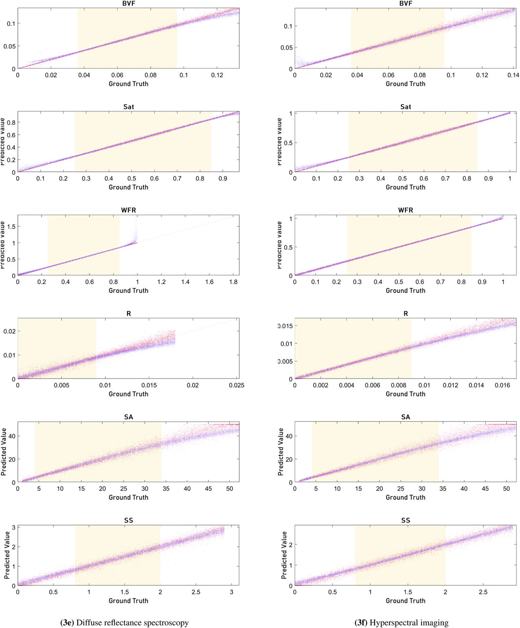
Figure 3. Figures showing the trends when plotting the ground truth (x-axis) against the estimated value (y-axis) for the trained network (magenta) and the diffusion model (purple). The left column shows results for DRS, and the right column shows results for HSI. The shaded yellow region represents the training range of optical properties, where regions outside the training range are used to evaluate network robustness for unexpected values. Parameters: blood volume fraction (BVF), blood saturation (SAT), average radius of blood vessels (R), water-fat ratio (WFR), scattering amplitude (SA), and scattering slope (SS).
The significance testing showed no significant differences for HSI and DRS, except for the radius (R) parameter in DRS compared between the network and diffusion theory, and ground truth and diffusion theory.
4 Discussion
From the results shown in Figures 2c,d the network estimates the optical properties as accurately as diffusion theory, in some cases outperforming the diffusion theory approach, but in general outperforms DT as seen from Table 3. From Table 3 it can be seen that the network has a median relative error of: 1.1% and 0.8% inside the training range and 4.2% and 2.2% outside of the training for the estimation of all the optical parameters for DRS and HSI respectively. The highest relative error in both being the average radius blood vessels (R). Both the network and diffusion theory are able to retrieve the optical properties from the synthetic spectra with only a small difference, as can be seen in Figures 2a,b. In Figures 2c,d it can also be seen that the median and distribution of groups do not differ greatly between the diffusion theory approximation and the network approximation, showing the ability of the network to approximate the values accurately.
To accurately evaluate the performance of the model the relative error is calculated. In Figures 2c,d it can be observed that the network has consistently lower relative errors for the optical properties compared to the diffusion theory approach. A consistent trend is observed for all the optical properties. The lower relative error might be due to there being non-unique combinations of parameters that can produce equal spectra when diffusion theory is used, especially for HSI where the error in general are higher for both the network and diffusion theory. When fitting these parameters from spectra, non-unique solutions for the parameters are possible. However, while fitting with diffusion theory requires explicit descriptions of the relationship between variables, as it is governed by the explicit equations and assumptions for light-transport in tissue; the neural network does not contain these explicit relationships between variables, possibly reducing the competition between these variables. As explained in the method section, to test the generalizability of the network outside the training range a second test set was used that contained values outside of the training range.
In Table 4, 5, significance testing revealed a noteworthy difference only for the average radius parameter—between diffusion theory and both the network and ground truth. However, the relative error (RE) analysis confirms high fidelity: the median RE is 0.13 for diffusion theory and 0.06 for the neural network, indicating no significant differences for most optical parameters between either method and the ground truth. These results mirror findings from Manojlović et al. (2023), who trained machine learning models on simulated hyperspectral data and achieved mean absolute errors (MAE) as low as 0.011 on real skin spectra, with inference times below 100 µs per spectrum. Manojlović et al. (2023) this demonstrates that models trained exclusively on simulated data can transfer effectively to real measurements.

Table 4. P-values for the different parameters between ground truth and the two methods in DRS, with all showing no significant difference except the average radius between diffusion theory and the network; and diffusion theory and the ground truth (shown in bold).

Table 5. P-values for the different parameters between ground truth and the two methods in HSI, with none showing any significant difference.
Moreover, our use of the RE metric is consistent with Claridge and Hidovic-Rowe (2014), who evaluated multispectral inversion accuracy in colon tissue using a similar error ratio, and reported normalized RMSD of 0.02 for ex-vivo parameter estimation based on model inversion (Claridge and Hidovic-Rowe, 2014). In summary, our neural network matches the accuracy benchmarks of both Manojlović et al. (2023) and Claridge and Hidovic-Rowe (2014), while delivering a substantial speed advantage over diffusion-theory-based fitting—achieving comparable accuracy with near real-time performance.
In Figure 3 figure scatter plots are shown for the performance of diffusion theory and the network on values outside of the training range. Here it can be seen that most parameters continue to be estimated well by the network outside of the bounds of the training data. For blood volume fraction (BVF), within the bounds of the training data, the network accurately predicts values that closely align with the ground truth. This is evidenced by the dense clustering of data points along the diagonal line representing perfect prediction. However, as the ground truth values extend beyond the training range, the network’s predictions start to diverge from the diagonal. This is most visible in the parameters describing the reduced scattering, where the spread of predicted values becomes broader and less consistent, indicating a decrease in prediction accuracy and robustness. The diffusion theory model, shown in purple, maintains a more stable and linear relationship even beyond the training range, as it is based on the fixed assumptions and relations of optical parameters. The radius of blood vessels (R) shows a similar trend to the BVF. Within the training range, the network’s predictions are tightly clustered along the diagonal, reflecting high accuracy. But outside this range, particularly in the HSI dataset, the predictions become increasingly scattered. This increased variability suggests that the neural network has reduced ability to generalize well beyond its training data for this parameter. This is most likely due to the limitations of the diffusion theory with the used wide-field approximation, as it results in more spectra that have non-unique solutions, making it harder for the network to maintain accuracy. The scattering amplitude (SA) parameter also displays non-linearity outside the training bounds. Within the range, the predictions are precise and closely match the ground truth. However, as the values move beyond this range, the network’s performance reduces.
To address these limitations, one potential approach is to expand the training dataset to include a more comprehensive range of data, simulating all possible ranges of optical properties. This would help ensure that the testing data rarely falls outside the training range, thereby improving the network’s generalization capabilities. Additionally, while diffusion theory provides a convenient and computationally efficient method for generating training data, its accuracy can be surpassed by more sophisticated simulation methods such as Monte Carlo simulations. These methods, though computationally intensive, could provide more accurate and reliable training data, thereby enhancing the network’s performance across a wider range of conditions. Therefore while the neural network demonstrates strong predictive capabilities within the bounds of its training data, its performance outside these bounds is less reliable for certain parameters, particularly in the HSI dataset. By expanding the training data and potentially integrating more sophisticated simulation techniques, the network’s robustness and accuracy can be significantly enhanced, leading to better predictions across a broader range of optical properties. Finally, as seen in Table 3, there is a significant speed-up for the processing of the data between network-based optical property retrieval and diffusion theory-based; with a speed increase from 2,486 s to 0.097 s for 30,000 spectra; with the largest time spent in the case of the network being the loading of the network itself; thus the scaling of the processing speed of the network is not linear. Furthermore, when performing the inference for the network on the GPU, which is not available for the fitting procedure, the speed up is even more signficant with an additional 2x speed up between CPU and GPU inference for the network. This speed increase might be important for real-time or time-sensitive applications where optical property retrieval is important. For the current model size and the expected size of the data input during inference, the primary time constraint lies in loading and unloading the model. During fitting, however, the time is primarily determined by the fitting speed of individual spectra. Consequently, in cases where the size of the input data is relatively small compared to the size of the model, there is a significant speed improvement. This improvement does not scale linearly with the size of the input data. In HSI, a small increase in the image resolution can greatly increase the number of spectra, thus greatly increasing the amount of time needed when fitting with conventional methods. For future research two main recommendations are given; firstly the method of data generation should better reflect the expected measured spectra; secondly, the trained network should be tested on measured data after training, to confirm the correct functioning of the network on measured data. For the first point, a different synthesis technique could be used, such as Monte Carlo modelling, where the tissue to be investigated could be better approximated. Furthermore, in future work the feed-forward network presented in this paper could be replaced with more complex network architectures that exploit additional information, such as spatial information in HSI or multiple source detector distances in DRS.
In conclusion, using a simple neural network in combination with synthetic training data allows both for DRS and HSI the correct retrieval of optical parameters faster and as accurate; given that the network is trained on the appropriate range of parameters in synthetic data.
In conclusion, using a simple neural network with synthetic training data enables fast and accurate retrieval of optical parameters for both DRS and HSI. By employing SNV normalization on the parameters, using a single unified architecture for both modalities, and explicitly testing performance outside the training range, this work demonstrates a robust and easily implementable approach. These contributions provide a foundation for translating deep learning-based optical property retrieval into practical clinical and experimental applications.
Data availability statement
The raw data supporting the conclusions of this article will be made available by the authors, without undue reservation.
Author contributions
MW: Formal Analysis, Conceptualization, Writing – review and editing, Methodology, Writing – original draft, Data curation, Visualization, Software. TN: Visualization, Data curation, Writing – original draft, Investigation, Writing – review and editing. TR: Conceptualization, Supervision, Writing – review and editing, Writing – original draft, Project administration. BD: Project administration, Writing – review and editing, Writing – original draft, Supervision.
Funding
The author(s) declare that financial support was received for the research and/or publication of this article. This work was supported by KWF Dutch Cancer Society project grant KWF 16687/2024.
Conflict of interest
The authors declare that the research was conducted in the absence of any commercial or financial relationships that could be construed as a potential conflict of interest.
Generative AI statement
The author(s) declare that no Generative AI was used in the creation of this manuscript.
Any alternative text (alt text) provided alongside figures in this article has been generated by Frontiers with the support of artificial intelligence and reasonable efforts have been made to ensure accuracy, including review by the authors wherever possible. If you identify any issues, please contact us.
Publisher’s note
All claims expressed in this article are solely those of the authors and do not necessarily represent those of their affiliated organizations, or those of the publisher, the editors and the reviewers. Any product that may be evaluated in this article, or claim that may be made by its manufacturer, is not guaranteed or endorsed by the publisher.
References
Adank, M. W., Fleischer, J. C., Dankelman, J., and Hendriks, B. H. W. (2018). Real-time oncological guidance using diffuse reflectance spectroscopy in electrosurgery: the effect of coagulation on tissue discrimination. J. Biomed. Opt. 23, 1. doi:10.1117/1.JBO.23.11.115004
Bahl, A., Segaud, S., Xie, Y., Shapey, J., Bergholt, M., and Vercauteren, T. (2023). A comparative study of analytical models of diffuse reflectance in homogeneous biological tissues: gelatin-based phantoms and monte carlo experiments. arXiv preprint ArXiv:2312.12935
Baltussen, E. J. M., Snaebjornsson, P., de Koning, S. G. B., Sterenborg, H. J. C. M., Aalbers, A. G. J., Kok, N., et al. (2017). Diffuse reflectance spectroscopy as a tool for real-time tissue assessment during colorectal cancer surgery. J. Biomed. Opt. 22, 1. doi:10.1117/1.jbo.22.10.106014
Baltussen, E. J. M., Kok, E. N. D., Brouwer de Koning, S. G., Sanders, J., Aalbers, A. G. J., Kok, N. F. M., et al. (2019). Hyperspectral imaging for tissue classification, a way toward smart laparoscopic colorectal surgery. J. Biomed. Opt. 24 (1), 1. doi:10.1117/1.jbo.24.1.016002
Barberio, M., Collins, T., Bencteux, V., Nkusi, R., Felli, E., Viola, M. G., et al. (2021). Deep learning analysis of in vivo hyperspectral images for automated intraoperative nerve detection. Diagnostics 11, 1508. doi:10.3390/diagnostics11081508
Brouwer de Koning, S. G., and Ruers, T. J. M. (2021). Tongue tumor detection in hyperspectral images using deep learning semantic segmentation. IEEE Trans. Biomed. Eng. 68, 938–945. doi:10.1109/TBME.2020.3026664
Claridge, E., and Hidovic-Rowe, D. (2014). Model based inversion for deriving maps of histological parameters characteristic of cancer from ex-vivo multispectral images of the colon. IEEE Trans. Med. Imaging 33, 822–835. doi:10.1109/TMI.2013.2290697
Coleman, T. F., and Li, Y. (1996). An interior trust region approach for nonlinear minimization subject to bounds. SIAM J. Optim. 6, 418–445. doi:10.1137/0806023
Cui, R., Yu, H., Xu, T., Xing, X., Cao, X., Yan, K., et al. (2022). Deep learning in medical hyperspectral images: a review. Sensors 22, 9790. doi:10.3390/s22249790
Currà, A., Gasbarrone, R., Cardillo, A., Trompetto, C., Fattapposta, F., Pierelli, F., et al. (2019). Near-infrared spectroscopy as a tool for in vivo analysis of human muscles. Sci. Rep. 9, 8623–14. doi:10.1038/s41598-019-44896-8
de Boer, L. L., Molenkamp, B. G., Bydlon, T. M., Hendriks, B. H., Wesseling, J., Sterenborg, H. J., et al. (2015). Fat/water ratios measured with diffuse reflectance spectroscopy to detect breast tumor boundaries. Breast Cancer Res. Treat. 152, 509–518. doi:10.1007/s10549-015-3487-z
De Boer, L. L., Bydlon, T. M., Van Duijnhoven, F., Vranken Peeters, M. J. T., Loo, C. E., Winter-Warnars, G. A., et al. (2018). Towards the use of diffuse reflectance spectroscopy for real-time in vivo detection of breast cancer during surgery. J. Transl. Med. 16, 367–14. doi:10.1186/s12967-018-1747-5
Farrell, T. J., Patterson, M. S., and Wilson, B. (1992). A diffusion theory model of spatially resolved, steady-state diffuse reflectance for the noninvasive determination of tissue optical properties in vivo. Med. Phys. 19, 879–888. doi:10.1118/1.596777
Fernandes, L., Carvalho, S., Carneiro, I., Henrique, R., Tuchin, V. V., Oliveira, H. P., et al. (2021). Diffuse reflectance and machine learning techniques to differentiate colorectal cancer ex vivo. Chaos An Interdiscip. J. Nonlinear Sci. 31, 053118. doi:10.1063/5.0052088
Flock, S. T., Patterson, M. S., Wilson, B. C., and Wyman, D. R. (1989). Monte Carlo modeling of light propagation in highly scattering tissues—I: model predictions and comparison with diffusion theory. IEEE Trans. Biomed. Eng. 36, 1162–1168. doi:10.1109/TBME.1989.1173624
Hokr, B. H., and Bixler, J. N. (2021). Machine learning estimation of tissue optical properties. Sci. Rep. 11, 6561. doi:10.1038/s41598-021-85994-w
Jacques, S. L. (2013). Optical properties of biological tissues: a review. Phys. Med. Biol. 58, R37–R61. doi:10.1088/0031-9155/58/11/R37
Livecchi, T. T., Jacques, S. L., Subhash, H. M., and Pierce, M. C. (2024). Hyperspectral imaging with deep learning for quantification of tissue hemoglobin, melanin, and scattering. J. Biomed. Opt. 29, 093507. doi:10.1117/1.JBO.29.9.093507
Lu, G., and Fei, B. (2014). Medical hyperspectral imaging: a review. J. Biomed. Opt. 19, 010901. doi:10.1117/1.jbo.19.1.010901
Mahmood, A., and Sears, M. (2021). Estimation of correlated signal-dependent noise statistics in hyperspectral images. Remote Sens. Lett. 12, 961–969. doi:10.1080/2150704x.2021.1946616
Manojlović, T., Toman̆č, T., Štajduhar, I., and Milanič, M. (2023). Rapid extraction of skin physiological parameters from hyperspectral images using machine learning. Appl. Intell. 53, 16519–16539. doi:10.1007/s10489-022-04327-0
Meola, J., Eismann, M. T., Moses, R. L., and Ash, J. N. (2011). Modeling and estimation of signal-dependent noise in hyperspectral imagery. Appl. Opt. 50, 3829. doi:10.1364/ao.50.003829
Nogueira, M. S., Maryam, S., Amissah, M., Lu, H., Lynch, N., Killeen, S., et al. (2021). Evaluation of wavelength ranges and tissue depth probed by diffuse reflectance spectroscopy for colorectal cancer detection. Sci. Rep. 11, 798–17. doi:10.1038/s41598-020-79517-2
Pertzborn, D., Bali, A., Mühlig, A., Von Eggeling, F., and Guntinas-Lichius, O. (2024). enHyperspectral imaging and evaluation of surgical margins: where do we stand? Curr. Opin. Otolaryngology and Head and Neck Surg. 32, 96–104. doi:10.1097/MOO.0000000000000957
Post, A. L., Jacques, S. L., Sterenborg, H. J. C. M., Faber, D. J., and van Leeuwen, T. G. (2017). Modeling subdiffusive light scattering by incorporating the tissue phase function and detector numerical aperture. J. Biomed. Opt. 22, 050501. doi:10.1117/1.jbo.22.5.050501
Power, A., Burda, Y., Edwards, H., Babuschkin, I., and Misra, V. (2022). Grokking: generalization beyond overfitting on small algorithmic datasets. arXiv preprint arXiv:2201.02177
Scarbrough, A., Chen, K., and Yu, B. (2024). Designing a use-error robust machine learning model for quantitative analysis of diffuse reflectance spectra. J. Biomed. Opt. 29, 015001. doi:10.1117/1.JBO.29.1.015001
Shi, Z., He, L., Suzuki, K., Nakamura, T., and Itoh, H. (2009). Survey on neural networks used for medical image processing. Int. J. Comput. Sci. 3, 86–100. Available online at: https://pubmed.ncbi.nlm.nih.gov/26740861/.
Veluponnar, D., Dashtbozorg, B., Jong, L.-J. S., Geldof, F., Da Silva Guimaraes, M., Vrancken Peeters, M.-J. T. F. D., et al. (2023). Diffuse reflectance spectroscopy for accurate margin assessment in breast-conserving surgeries: importance of an optimal number of fibers. Biomed. Opt. Express 14, 4017. doi:10.1364/BOE.493179
Wang, L. V., Jacques, S. L., and Zheng, L. (2005). Monte Carlo-based inverse model for calculating tissue optical properties Part I: theory and validation on synthetic phantoms. Appl. Opt. 45, 1062–1071. doi:10.1364/AO.45.001062
Witteveen, M., Faber, D. J., Sterenborg, H. J. C. M., Ruers, T. J. M., van Leeuwen, T. G., and Post, A. L. (2022a). Opportunities and pitfalls in (sub)diffuse reflectance spectroscopy. Front. Photonics 3, 964719–19. doi:10.3389/fphot.2022.964719
Witteveen, M., Sterenborg, H. J. C. M., van Leeuwen, T. G., Aalders, M. C. G., Ruers, T. J. M., and Post, A. L. (2022b). Comparison of preprocessing techniques to reduce nontissue-related variations in hyperspectral reflectance imaging. J. Biomed. Opt. 27, 106003–106024. doi:10.1117/1.JBO.27.10.106003
Keywords: diffuse reflectance spectroscopy, hyperspectral imaging, optical property retrieval, diffusion theory, deep learning, physiological parameters, simulated training data, biomedical optics
Citation: Witteveen M, Natali T, Ruers TJM and Dashtbozorg B (2025) Physics inspired neural network for optical property retrieval from diffuse reflectance. Front. Photonics 6:1634102. doi: 10.3389/fphot.2025.1634102
Received: 23 May 2025; Accepted: 01 September 2025;
Published: 25 September 2025.
Edited by:
Wenfeng Xia, King’s College London, United KingdomReviewed by:
Yijing Xie, King’s College London, United KingdomSinem Uysal, Ankara Science University, Türkiye
Copyright © 2025 Witteveen, Natali, Ruers and Dashtbozorg. This is an open-access article distributed under the terms of the Creative Commons Attribution License (CC BY). The use, distribution or reproduction in other forums is permitted, provided the original author(s) and the copyright owner(s) are credited and that the original publication in this journal is cited, in accordance with accepted academic practice. No use, distribution or reproduction is permitted which does not comply with these terms.
*Correspondence: Mark Witteveen, bWEud2l0dGV2ZWVuQG5raS5ubA==