Abstract
Dry weight (DW) is an important dialysis index for patients with end-stage renal disease. It can guide clinical hemodialysis. Brain natriuretic peptide, chest computed tomography image, ultrasound, and bioelectrical impedance analysis are key indicators (multisource information) for assessing DW. By these approaches, a trial-and-error method (traditional measurement method) is employed to assess DW. The assessment of clinician is time-consuming. In this study, we developed a method based on artificial intelligence technology to estimate patient DW. Based on the conventional radial basis function neural (RBFN) network, we propose a multiple Laplacian-regularized RBFN (MLapRBFN) model to predict DW of patient. Compared with other model and body composition monitor, our method achieves the lowest value (1.3226) of root mean square error. In Bland-Altman analysis of MLapRBFN, the number of out agreement interval is least (17 samples). MLapRBFN integrates multiple Laplace regularization terms, and employs an efficient iterative algorithm to solve the model. The ratio of out agreement interval is 3.57%, which is lower than 5%. Therefore, our method can be tentatively applied for clinical evaluation of DW in hemodialysis patients.
Introduction
Dry weight (DW) refers to a patient’s target weight after the end of dialysis (Grassmann et al., 2000; Wabel et al., 2009). After removing excess water from the body, the patient had no facial swelling, wheezing or sitting breathing, edema of both lower limbs, and distended jugular vein (Alexiadis et al., 2016). The patient’s blood pressure, heart rate, breathing, and other vital signs are stable. There are individual differences in the specific value of DW. Good dry weight control can effectively reduce adverse reactions during dialysis. At present, the DW of hemodialysis patients is mainly evaluated by clinical means. This method is labor-intensive and time-consuming, and requires repeated use of various clinical instruments and biological indicators to complete the evaluation. In the past 10 years, a measuring instrument based on human bioelectrical impedance analysis (BIA), called body composition monitor (BCM) (Jiang et al., 2017), has been accurately determining the DW of patients. The above methods require professionals and cannot be processed on a large scale.
In recent years, artificial intelligence technology has been widely utilized in the biomedical field (Chen et al., 2019; Cheng et al., 2019; Lin, 2020; Zhang, 2020; Hu et al., 2021a). Artificial neural networks (ANNs) based on back propagation (BP) were employed to evaluate the total water volume of hemodialysis patients. Compared with conventional clinical calculation equations (Chiu et al., 2005), the ANNs obtained better results. Deep learning (Dao et al., 2021; Lv et al., 2021a,b) also made a great contribution to the clinic, including skin cancer (Esteva et al., 2017), breast cancer (Liu J. et al., 2021), and brain diseases (Liu G. et al., 2018; Liu et al., 2019; Bi et al., 2020; Hu et al., 2020, 2021a,b). In biological field, machine learning has been widely used to solve biological problems, including O-GlcNAcylation site prediction (Jia et al., 2018), microbiology analysis (Qu et al., 2019), microRNAs and cancer association prediction (Zeng et al., 2018), lncRNAs (Cheng et al., 2016; Deng et al., 2021), CircRNAs (Fang et al., 2019; Zhao et al., 2019), DNA methylation site (Wei et al., 2018b; Zou et al., 2019; Dai et al., 2020), osteoporosis diagnoses (Su et al., 2020b), function prediction of proteins (Wei et al., 2018a; Wang H. et al., 2019; Deng et al., 2020b; Ding et al., 2020a; Su et al., 2020a), nucleotide binding sites (Ding et al., 2021b), drug complex network analysis (Ding et al., 2019, 2020b,a; Deng et al., 2020a; Han et al., 2021; Liu H. et al., 2021), protein remote homology (Liu B. et al., 2018), electron transport proteins (Ru et al., 2019), and cell-specific replication.
In this study, we proposed a novel predictive model based on radial basis function neural network (RBFN). Different from RBFN, multiple Laplacian-regularized RBFN (MLapRBFN) is a multi-view Laplacian regularized model with L2,1-norm, which introduces multiple graph regular items. The Laplacian regular items consider the topological relationship between each patient.
Materials and Methods
Materials
The data set of this study came from the hemodialysis center of Wuxi and the northern Jiangsu People’s Hospital. Our study was approved by the ethics committees (Nos. 2018KY-001 and KYLLKS201813). There are a total of 476 hemodialysis patients. These patients meet the following conditions: over 18 years old; more than 3 months end-stage renal disease (ESRD) and maintenance hemodialysis; diseases such as metal implants, infections, heart failure, disability, pregnancy, and edema, do not appear in the patient population. DW is determined by clinical scoring, which is based on brain natriuretic peptide (BNP), chest computed tomography (CT) image, ultrasound, and bioelectrical impedance analysis (BIA). In addition, age, gender, diastolic blood pressure (DBP), systolic blood pressure (SBP), years of dialysis (YD), heart rate (HR), and body mass index (BMI) are employed to construct our model. The summary of information is shown in Table 1. This study is a retrospective study, and feature of patient is easy to obtain. We hope to provide patients with a non-invasive dry weight assessment method through machine learning models.
TABLE 1
| Feature | Value | r * |
| Gender (males/females) | 312/164 | –0.4489 |
| Age (years) | 54.17 ± 14.22 | –0.2341 |
| BMI | 22.96 ± 2.95 | 0.9558 |
| HR (times/min) | 73.41 ± 8.92 | 0.1862 |
| DBP (mmHg) | 88.32 ± 19.56 | –0.1249 |
| SBP (mmHg) | 150.64 ± 29.36 | –0.1739 |
| YD (years) | 5.97 ± 3.22 | –0.1069 |
She summary information of patients.
*Denotes correlation coefficient between individual variables and dry weight value.
Radial Basis Function Network
The RBF neural network (Park and Sandberg, 1990) is composed of an input layer, a hidden layer, and an output layer, and is shown in Figure 1. The feature of the hemodialysis patient can be fed into the RBF network for processing. Suppose that there are N samples containing d variables ({xi, yi}, i = 1, 2, …, N). The output is yi ∈ R1×q and input data xi ∈ R1×d. In Figure 1, the RBF network has three layers, which are the input, hidden, and output layers. The transformation from the input space to the hidden layer space is non-linear, and the transformation between the hidden layer and the output layer is linear. The fundamental of the RBFN is the RBF is the “base” of the hidden unit. The vector of input layer can be mapped to the space of the hidden layer without weight connection. The mapping relationship is determined with center point of hidden unit. In Figure 1, the number of hidden layer nodes is p (p center points). The activation function of the RBF neural network can be represented as:
where xi is a feature vector of sample, cj, j ∈ {1, 2, …, p} is the vector of j-th center point, and σ is the width parameter of the function, which controls the radial range of the function. RBFN can be represented as:
where matrix Φ ∈ RN×p is the output of the hidden nodes. W ∈ Rp×q is the weight matrix between output and hidden nodes. Y ∈ RN×q is the matrix of dependent variable. Φ ∈ RN×p and W ∈ Rp×q can be represented as:
FIGURE 1
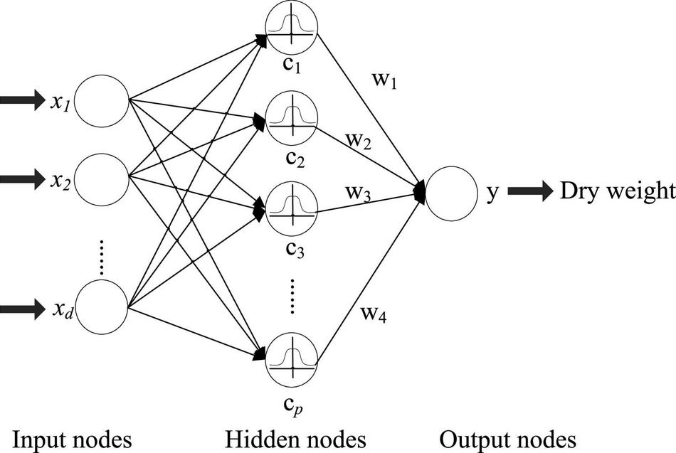
Topological structure of the radial basis function (RBF) network.
To train RBFN, 3 parameters should be solved: the center points of the basis function (cj ∈ R1×d, j ∈ {1, 2, …, p}), width (σ), and weight matrix between the output and hidden layer (W ∈ Rp×q). In most cases, the self-organized selection center learning method is used: (1) unsupervised learning process, solving the center points and width of RBF, (2) supervised learning process, solving the weights W ∈ Rp×q. First, select p centers for k-means clustering (p clusters). For the radial basis of the Gaussian kernel function, the width is solved by the formula:
where σmax is the maximum distance between the selected center points.
For W ∈ Rp × q, the RBF network can be represented as:
The gradient of Eq. 6 can be set as 0:
For a new test sample xnew, we can estimate as:
where Φnew = (ϕ (xnew, c1), ϕ (xnew, c2), …, ϕ (xnew, cp))1 × p.
Proposed Model of Multiple Laplacian-Regularized RBF Network
To further improve the generalization performance of the RBF network, a multi-view Laplacian-regularized RBF network is proposed. The unsupervised process of the first stage remains unchanged; we mainly improve the model in the second part. The objective function of Eq. 6 is revised as:
where λ1 and λ2 denote the parameters of Laplacian and L2, 1-norm term. L2, 1-norm can be used to obtain a sparser solution during the training process, which makes the model more robust. ρ > 1, which is used to prevent the extreme situations of ηv = 0 (or ηv = 1). Lv ∈ RN×N is the Laplacian matrix, which is employed to represent the manifold of samples. V is the number of views. Lv is built by heat kernel matrix Sv ∈ RN×N:
In our study, we employ the following functions to construct the heat kernel matrix:
where γ is a constant, and we set it as 1.
Optimization
The third term of cannot be diversified, so Eq. 9 is converted into:
where G ∈ Rp×p is a diagonal matrix, and i-th is an element:
Since there are multiple variables (W, ηv) that need to be optimized, we first fix ηv and optimize W. We initialize , and get the fused matrix . Equation 12 can be written as:
We obtain the derivative of formula (14) for variable W:
Then, we fix the variant W and optimize ηv, v = 1, 2, …, V, which is related to:
The above formula can be converted to a Lagrange function:
We set ηv and ξ to 0:
where ηv can be estimated by:
The process of MLapRBFN is listed in Algorithm 1 and Figure 2.
Algorithm 1: Algorithm of multiple Laplacian-regularized RBFN (MLapRBFN).
Require: Training set {xi, yi}, i = 1, 2, …, N, new samples{xnew, j}, j = 1, 2, …, M, the hidden layer nodes (p), the iterations tmax, parameters of λ1and λ2;
Ensure: The predictive values of
(1) Using k-means to select p centers and width (σ ) for RBF function. Calculating the W (training set) and Laplacian matrices Lv, v = 1, 2, …, V by Eqs 1, 10, and 11. Initializing ;
(2) Setting t = 0, estimate the initial W(0) with Eq. 7;
Repeat
(3) Update the G(t + 1)with
(4) Update W(t + 1) via Eq. 15d;
(5) Update via Eq. 19;
(6) Calculating
until t > tmax;
(7) Calculate the output matrix Φnew(test set);
(8) Predict {ynew, j}, j = 1, 2, …, M by .
FIGURE 2
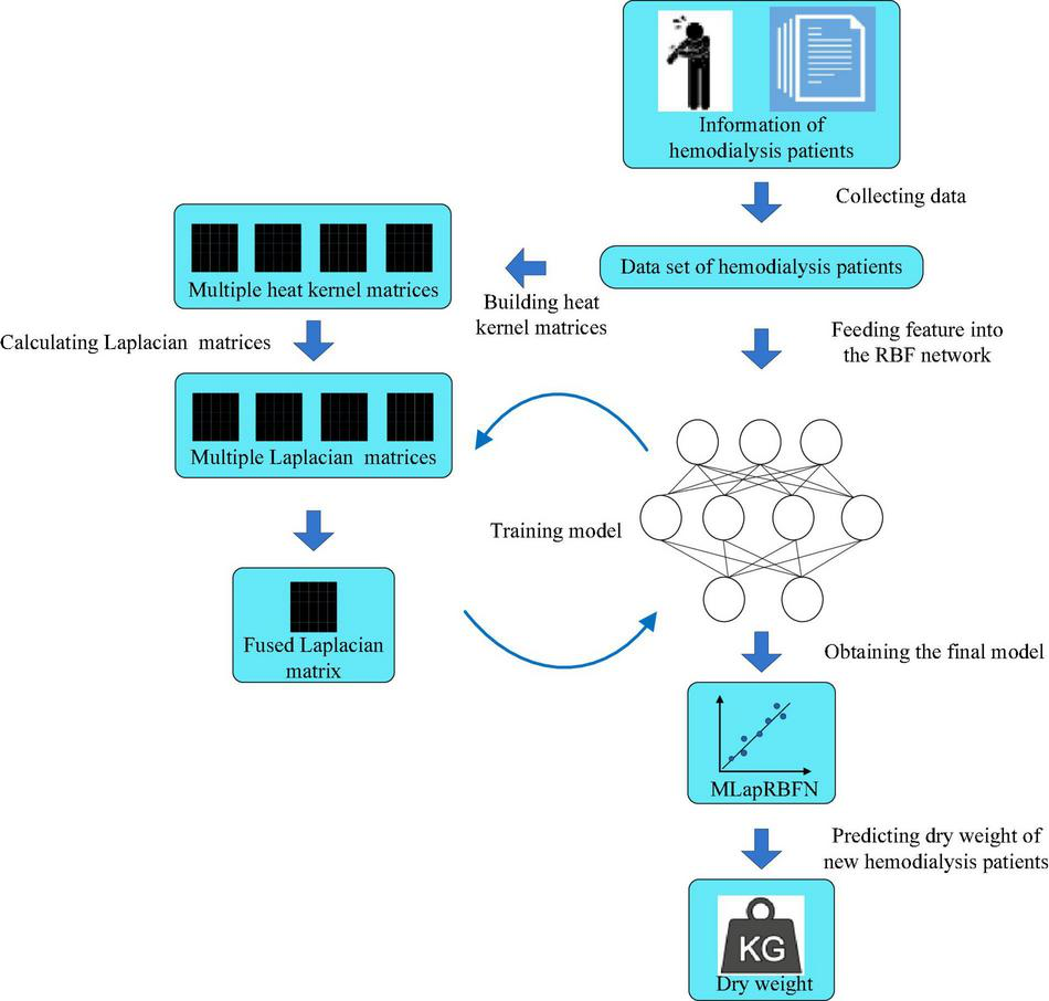
Flow chart of multiple Laplacian-regularized RBF network (MLapRBFN).
Results and Discussion
In this section, we perform 10-fold cross-validation (10-CV) to test the predictive performance of different models, the BCM device, multiple kernel support vector regression (MKSVR), linear regression (LR), back propagation-based artificial neural network [ANN (BP)], and multi-kernel ridge regression (MKRR).
Evaluation Measurements
Some traditional assessment methods include correlation coefficient (R), R square, root mean square error (RMSE), empirical cumulative distribution plot (ECDP), and Bland–Altman analysis. In particular, The Bland–Altman analysis usually can evaluate the agreement between two methods, and determines whether the two methods can be replaced with each other.
Selection of Optimal Parameters
We obtain the optimal model parameters, such as the number of hidden layer nodes (the number of clusters), regularization parameters, and number of optimization iterations. First, we fix the number of iterations (tmax = 10) and regularization coefficients (λ1 = 20, λ2 = 20), and adjust the number of hidden layer neurons. In Figure 3A, we test the number of nodes from 10 to 250 with step of 10. After adding 140 neuron nodes, RMSE tends to be flat. In addition, the RMSE also tends to remain unchanged (minimum) after 10 iterations (Figure 3B). Finally, we get the number of hidden layer nodes as 140 and times of iteration as 10, and adjust the regularization coefficient. The results are shown in Figure 4, and the optimal coefficients are .
FIGURE 3
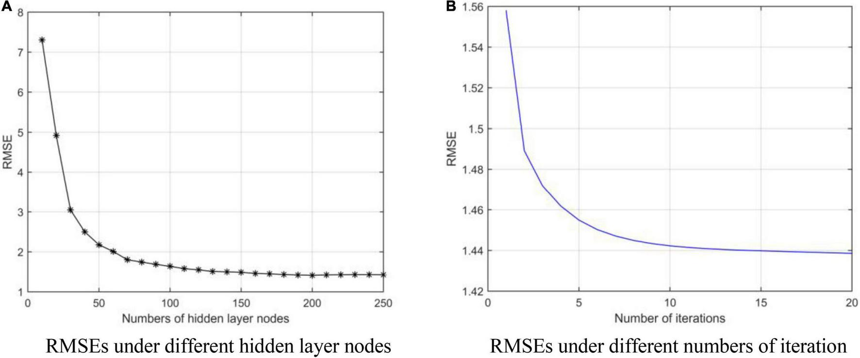
RMSEs under different parameters. (A) Root mean square errors (RMSEs) under different hidden layer nodes. (B) RMSEs under different numbers of iteration.
FIGURE 4
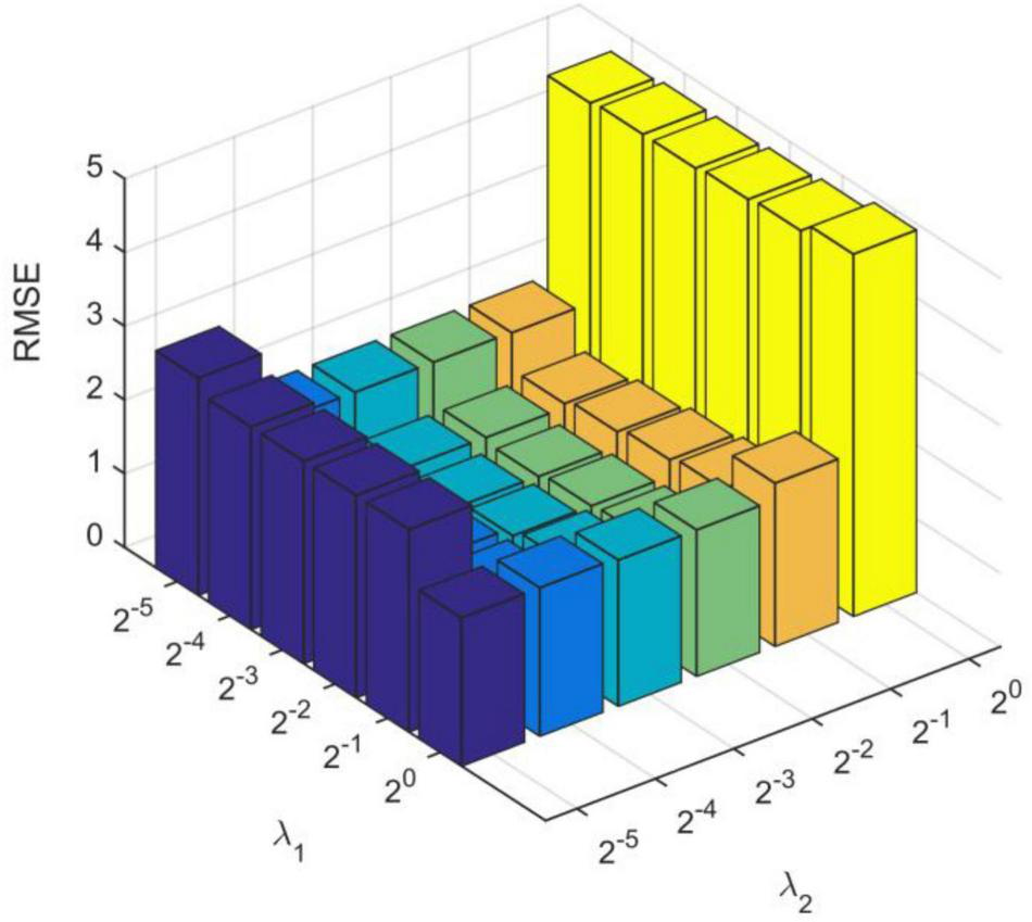
Root mean square errors under different regularization coefficients.
Comparison With Other Existing Models
We compare our model with other existing machine learning methods (Guo et al., 2021), which include multi-kernel ridge regression (MKRR), multiple kernel support vector regression (MKSVR), artificial neural network (ANN), linear regression (LR), and BCM measuring instrument. The gold standard is clinical dry weight. In Table 2, our method (MLapRBFN) is better than the ordinary RBF neural network (RBFN) model. The R and R squared have the highest values of 0.9511 and 0.9432, respectively. In addition, the RMSE of MLapRBFN reaches its lowest value (1.3226). In Table 2 and Figure 5, we can see that our method has the smallest ECDP range (from −3.8174 to 3.4383). The multiple Laplacian regularized RBFN model has multiple graphs for different heat kernels, which contain different information. To effectively integrate each graph of feature into one graph, multi-view learning (MVL) is employed to estimate the weight of each graph. Each graph has different contribution for the model.
TABLE 2
| Method | R | R Squared | RMSE | Empirical cumulative distribution plot |
||
| Highest value | Lowest value | Median value | ||||
| MKSVR* | 0.9412 | 0.9321 | 1.3817 | 4.3962 | −4.1273 | 0.0082 |
| MKRR* | 0.9399 | 0.9289 | 1.5015 | 4.9227 | −4.2604 | 0.1104 |
| ANN (BP)* | 0.9398 | 0.9295 | 1.4794 | 7.3661 | −4.7447 | 0.1324 |
| LR* | 0.9403 | 0.9308 | 1.4335 | 4.2524 | −.4014 | 0.1418 |
| BCM* | 0.9473 | 0.9137 | 1.9694 | 3.2235 | −6.2776 | −.9863 |
| RBFN | 0.9410 | 0.9302 | 1.4514 | 4.9018 | −3.9376 | 0.0966 |
| MLapRBFN (our method) | 0.9511 | 0.9432 | 1.3226 | 3.4383 | -3.8174 | 0.0822 |
Comparison with other methods (10-CV).
*The results are from previous work of MKSVR. Bold values represents the best performance for each column.
FIGURE 5
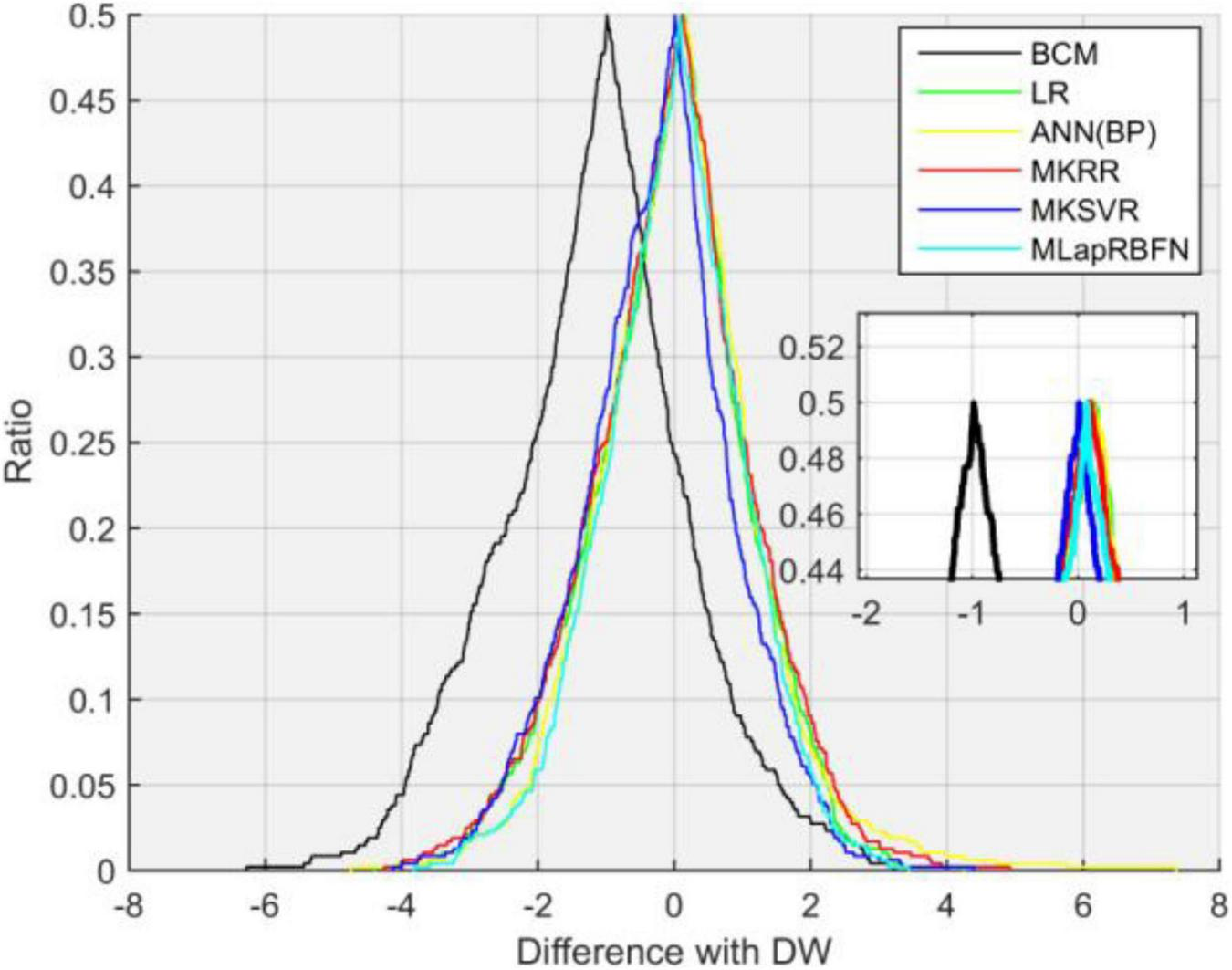
Folded empirical cumulative distribution curves of six methods.
Bland-Altman Analysis
In this section, we employ a Bland–Altman plot to further evaluate the regression error of different models. In Figure 6 and Table 3, several models evaluate the agreement with clinical DW. MLapRBFN achieves the smallest range of -0.2413 to 0.1601 (95% confidence interval). What is more, the number (ratio) of out agreement interval is the key indicator to evaluate whether the two methods are equivalent. For the predictive models, the number (ratio) should be all less than 24 (5%). In Table 3, all the predictive models meet this standard. In particular, our method obtains the least number (ratio) of 17 (3.57%). If 95% of the samples are in agreement range, the predictive models are clinically acceptable. It can be seen that our method can replace clinical methods.
FIGURE 6
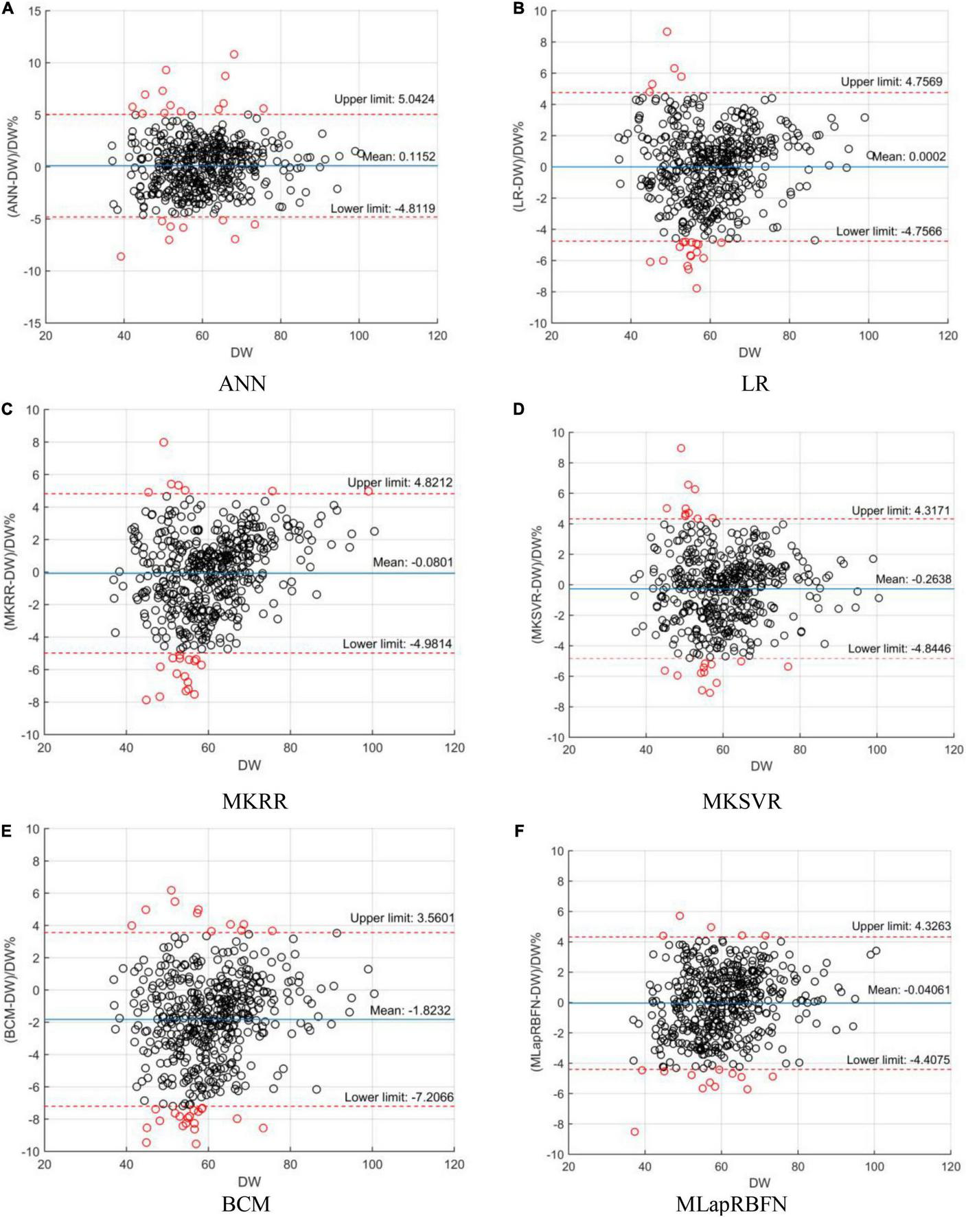
Bland–Altman plot analysis. (A) ANN, (B) LR, (C) MKRR, (D) MKSVR, (E) BCM, and (F) MLapRBFN.
TABLE 3
| Model | Differences with DW (%) |
Limits of agreement (%) |
||||
| Mean | SD | 95% confidence interval | Lower limit | Upper limit | Number (ratio) of out agreement interval | |
| MKSVR* | −0.2638 | 2.3372 | −0.4743 to -0.05329 | −4.8446 | 4.3171 | 22/476 (4.62%) |
| MKRR* | −0.0801 | 2.5007 | −0.3053 to 0.1451 | −4.9814 | 4.8212 | 23/476 (4.83%) |
| ANN (BP)* | 0.1152 | 2.5139 | −0.1112 to 0.3416 | −4.8119 | 5.0424 | 22/476 (4.62%) |
| LR* | 0.0002 | 2.4269 | −0.2184 to 0.2187 | −4.7566 | 4.7569 | 21/476 (4.41%) |
| BCM* | −1.8232 | 2.7466 | −2.0706 to −1.5759 | −7.2066 | 3.5601 | 30/476 (6.30%) |
| MLapRBFN (our method) | −0.04061 | 2.2280 | −0.2413 to 0.1601 | −4.4075 | 4.3263 | 17/476 (3.57%) |
Bland–Altman plot analysis of the models.
*The results are from previous work of MKSVR (Guo et al., 2021).
Conclusion
The limitations of BCM and clinical are time-consuming and laborious. In our study, a MLapRBFN method is developed to predict the DW of hemodialysis patients. Different from standard RBFN, our method contains multiple Laplace regularization terms, and uses an efficient iterative algorithm to solve the model. MKRR, LR, MKSVR, and ANN are compared with our model. Bland-Altman analysis and RMSE are the main evaluation methods. In the Bland-Altman analysis of MLapRBFN, the number of out agreement interval is the least (17 samples).
In the fields of medicine (Esteva et al., 2017; Xiao et al., 2017; Hu et al., 2018; Deng et al., 2019; Huang et al., 2020; Zhou et al., 2020; Yang H. et al., 2021), pharmacy (Wang et al., 2020), and biology (Wei et al., 2014, 2017, 2019; Fajila, 2019; Wang Y. et al., 2019; Wang et al., 2021; Yang C. et al., 2021; Zou et al., 2021), artificial intelligence technology has solved lots of predictive tasks. In future studies, more data of hemodialysis patients will be collected, and a deep neural network (Dao et al., 2020a,b; Lv et al., 2020) with stronger representation ability to accurately estimate the DW of hemodialysis patients will be built.
Publisher’s Note
All claims expressed in this article are solely those of the authors and do not necessarily represent those of their affiliated organizations, or those of the publisher, the editors and the reviewers. Any product that may be evaluated in this article, or claim that may be made by its manufacturer, is not guaranteed or endorsed by the publisher.
Statements
Data availability statement
The original contributions presented in the study are included in the article/supplementary material, further inquiries can be directed to the corresponding authors.
Ethics statement
The studies involving human participants were reviewed and approved by the experimental protocol was established and approved by the Human Ethics Committee (Wuxi and Northern Jiangsu People’s Hospital Ethics Committee). The ethical approval numbers are 2018KY-001 and KYLLKS201813. The patients/participants provided their written informed consent to participate in this study.
Author contributions
XG and WZ did the experiments and wrote the manuscript. YD, CL, and XG designed the method. YY, YZ, AD, QL, and YC revised the manuscript. All authors have read and approved the final manuscript.
Funding
This study was supported by the National Natural Science Foundation of China (NSFC 62172076 and 61902271), Natural Science Research Project of Jiangsu Higher Education Institutions of China (19KJB520014), Special Science Foundation of Quzhou (2021D004), and Research Project of Wuxi Nursing Association (No. Q202102).
Conflict of interest
The authors declare that the research was conducted in the absence of any commercial or financial relationships that could be construed as a potential conflict of interest.
References
1
Alexiadis G. Panagoutsos S. Roumeliotis S. Stibiris I. Passadakis P. (2016). Comparison of multiple fluid status assessment methods in patients on chronic hemodialysis.Int. Urol. Nephrol.491–8.
2
Bi X.-A. Liu Y. Xie Y. Hu X. Jiang Q. (2020). Morbigenous brain region and gene detection with a genetically evolved random neural network cluster approach in late mild cognitive impairment.Bioinformatics362561–2568. 10.1093/bioinformatics/btz967
3
Chen X. G. Shi W. W. Deng L. (2019). Prediction of disease comorbidity using hetesim scores based on multiple heterogeneous networks.Curr. Gene. Ther.19232–241. 10.2174/1566523219666190917155959
4
Cheng L. Shi H. Wang Z. Hu Y. Yang H. Zhou C. et al (2016). IntNetLncSim: an integrative network analysis method to infer human lncRNA functional similarity.Oncotarget747864–47874. 10.18632/oncotarget.10012
5
Cheng L. Zhuang H. Ju H. Yang S. Han J. Tan R. et al (2019). Exposing the causal effect of body mass index on the risk of type 2 diabetes mellitus: a mendelian randomization study.Front. Genet.2019:10.
6
Chiu J. S. Chong C. F. Lin Y. F. Wu C. C. Wang Y. F. Li Y. C. (2005). Applying an artificial neural network to predict total body water in hemodialysis patients.Am. J. Nephrol.25507–513. 10.1159/000088279
7
Dai C. Feng P. Cui L. Su R. Chen W. Wei L. (2020). Iterative feature representation algorithm to improve the predictive performance of N7-methylguanosine sites.Brief. Bioinform.22:278. 10.1093/bib/bbaa278
8
Dao F.-Y. Lv H. Su W. Sun Z.-J. Huang Q.-L. Lin H. (2021). iDHS-Deep: an integrated tool for predicting DNase I hypersensitive sites by deep neural network.Brief. Bioinform.22:47. 10.1093/bib/bbab047
9
Dao F.-Y. Lv H. Zhang D. Zhang Z.-M. Liu L. Lin H. (2020a). DeepYY1: a deep learning approach to identify YY1-mediated chromatin loops.Brief. Bioinform.22:356. 10.1093/bib/bbaa356
10
Dao F.-Y. Lv H. Zulfiqar H. Yang H. Su W. Gao H. et al (2020b). A computational platform to identify origins of replication sites in eukaryotes.Brief. Bioinform.221940–1950. 10.1093/bib/bbaa017
11
Deng L. Cai Y. Zhang W. Yang W. Gao B. Liu H. (2020a). Pathway-guided deep neural network toward interpretable and predictive modeling of drug sensitivity.J. Chem. Inform. Model.604497–4505. 10.1021/acs.jcim.0c00331
12
Deng L. Li W. Zhang J. (2021). LDAH2V: exploring meta-paths across multiple networks for lncRNA-disease association prediction.IEEE/ACM Trans. Comput. Biol. Bioinform.181572–1581. 10.1109/TCBB.2019.2946257
13
Deng L. Liu Y. Shi Y. Zhang W. Yang C. Liu H. (2020b). Deep neural networks for inferring binding sites of RNA-binding proteins by using distributed representations of RNA primary sequence and secondary structure.BMC Genomics21:866. 10.1186/s12864-020-07239-w
14
Deng L. Ye D. Zhao J. Zhang J. (2019). MultiSourcDSim: an integrated approach for exploring disease similarity.BMC Med. Inf. Decis. Mak.19:269. 10.1186/s12911-019-0968-8
15
Ding Y. Tang J. Guo F. (2019). Identification of drug-side effect association via multiple information integration with centered kernel alignment.Neurocomputing325211–224.
16
Ding Y. Tang J. Guo F. (2020a). Human protein subcellular localization identification via fuzzy model on kernelized neighborhood representation.Appl. Soft. Comput.96:106596.
17
Ding Y. Tang J. Guo F. (2020b). Identification of drug–target interactions via dual laplacian regularized least squares with multiple kernel fusion.Knowl. Based Syst.204:106254.
18
Ding Y. Tang J. Guo F. (2021a). Identification of drug-target interactions via multi-view graph regularized link propagation model.Neurocomputing461618–631. 10.1016/j.neucom.2021.05.100
19
Ding Y. Yang C. Tang J. Guo F. (2021b). Identification of protein-nucleotide binding residues via graph regularized k-local hyperplane distance nearest neighbor model.Appl. Intell.2021:2737.
20
Esteva A. Kuprel B. Novoa R. A. Ko J. Swetter S. M. Blau H. M. et al (2017). Dermatologist-level classification of skin cancer with deep neural networks.Nature542115–118.
21
Fajila M. N. F. (2019). Gene subset selection for leukemia classification using microarray data.Curr. Bioinform.14353–358.
22
Fang S. Pan J. C. Zhou C. W. Tian H. He J. X. Shen W. Y. et al (2019). Circular RNAs serve as novel biomarkers and therapeutic targets in cancers.Curr. Gene. Ther.19125–133.
23
Grassmann A. Uhlenbusch-Körwer I. Bonnie-Schorn E. Vienken J. (2000). Composition and management of hemodialysis fluids.Rockledge, FL: Pabst Science Publishers.
24
Guo X. Y. Zhou W. Shi B. Wang X. H. Du A. Y. Ding Y. J. et al (2021). An efficient multiple kernel support vector regression model for assessing dry weight of hemodialysis patients.Curr. Bioinform.16284–293.
25
Han X. Kong Q. Liu C. Cheng L. Han J. (2021). SubtypeDrug: a software package for prioritization of candidate cancer subtype-specific drugs.Bioinformatics2021:11. 10.1093/bioinformatics/btab011
26
Hu Y. Qiu S. Cheng L. (2021a). Integration of multiple-omics data to analyze the population-specific differences for coronary artery disease.Comput. Math. Methods Med.2021:7036592. 10.1155/2021/7036592
27
Hu Y. Sun J. Y. Zhang Y. Zhang H. Gao S. Wang T. et al (2021b). rs1990622 variant associates with Alzheimer’s disease and regulates TMEM106B expression in human brain tissues.BMC Med.19:11. 10.1186/s12916-020-01883-5
28
Hu Y. Zhang H. Liu B. Gao S. Wang T. Han Z. (2020). rs34331204 regulates TSPAN13 expression and contributes to Alzheimer’s disease with sex differences.Brain143:e95.
29
Hu Y. Zhao T. Zang T. Zhang Y. Cheng L. (2018). Identification of alzheimer’s disease-related genes based on data integration method.Front. Genet.9:703.
30
Huang Y. Yuan K. Tang M. Yue J. Bao L. Wu S. et al (2020). Melatonin inhibiting the survival of human gastric cancer cells under ER stress involving autophagy and Ras-Raf-MAPK signalling.J. Cell Mol. Med.20201–13. 10.1111/jcmm.16237
31
Jia C. Zuo Y. Zou Q. (2018). O-GlcNAcPRED-II: an integrated classification algorithm for identifying O-GlcNAcylation sites based on fuzzy undersampling and a K-means PCA oversampling technique.Bioinformatics342029–2036. 10.1093/bioinformatics/bty039
32
Jiang C. Patel S. Moses A. DeVita M. V. Michelis M. F. (2017). Use of lung ultrasonography to determine the accuracy of clinically estimated dry weight in chronic hemodialysis patients.Int. Urol. Nephrol.492223–2230.
33
Lin H. (2020). Development and application of artificial intelligence methods in biological and medical data.Curr. Bioinform.15515–516. 10.2174/157489361506200610112345
34
Liu B. Jiang S. Zou Q. (2018b). HITS-PR-HHblits: protein remote homology detection by combining pagerank and hyperlink-induced topic search.Brief. Bioinform.21:104. 10.1093/bib/bby104
35
Liu G. Hu Y. Han Z. Jin S. Jiang Q. (2019). Genetic variant rs17185536 regulates SIM1 gene expression in human brain hypothalamus.Proc. Nat. Acad. Sci.1163347–3348. 10.1073/pnas.1821550116
36
Liu G. Jin S. Hu Y. Jiang Q. (2018a). Disease status affects the association between rs4813620 and the expression of Alzheimer’s disease susceptibility gene TRIB3.Proc. Nat. Acad. Sci.115E10519–E10520. 10.1073/pnas.1812975115
37
Liu H. Zhang W. Zou B. Wang J. Deng Y. Deng L. (2021a). Correction to ‘DrugCombDB: a comprehensive database of drug combinations toward the discovery of combinatorial therapy.Nucleic Acids Res.48:1007. 10.1093/nar/gkab836
38
Liu J. Su R. Zhang J. Wei L. (2021b). Classification and gene selection of triple-negative breast cancer subtype embedding gene connectivity matrix in deep neural network.Brief. Bioinform.22:bbaa395. 10.1093/bib/bbaa395
39
Lv H. Dao F.-Y. Guan Z.-X. Yang H. Li Y.-W. Lin H. (2020). Deep-Kcr: accurate detection of lysine crotonylation sites using deep learning method.Brief. Bioinform.22:255. 10.1093/bib/bbaa255
40
Lv H. Dao F.-Y. Zulfiqar H. Lin H. (2021a). DeepIPs: comprehensive assessment and computational identification of phosphorylation sites of SARS-CoV-2 infection using a deep learning-based approach.Brief. Bioinform.22:244. 10.1093/bib/bbab244
41
Lv H. Dao F.-Y. Zulfiqar H. Su W. Ding H. Liu L. et al (2021b). A sequence-based deep learning approach to predict CTCF-mediated chromatin loop.Brief. Bioinform.22:31. 10.1093/bib/bbab031
42
Park J. Sandberg I. W. (1990). Universal approximation using radial basis function networks.Neural Comput.3246–257. 10.1162/neco.1991.3.2.246
43
Qu K. Guo F. Liu X. Zou Q. (2019). Application of machine learning in microbiology.Front. Microbiol.10:827.
44
Ru X. Li L. Zou Q. (2019). Incorporating distance-based top-n-gram and random forest to identify electron transport proteins.J. Prot. Res.182931–2939. 10.1021/acs.jproteome.9b00250
45
Su R. He L. Liu T. Liu X. Wei L. (2020a). Protein subcellular localization based on deep image features and criterion learning strategy.Brief. Bioinform.22:313. 10.1093/bib/bbaa313
46
Su R. Liu T. Sun C. Jin Q. Jennane R. Wei L. (2020b). Fusing convolutional neural network features with hand-crafted features for osteoporosis diagnoses.Neurocomputing385300–309.
47
Wabel P. Chamney P. Moissl U. Jirka T. (2009). Importance of whole-body bioimpedance spectroscopy for the management of fluid balance.Blood Purif.2775–80. 10.1159/000167013
48
Wang H. Ding Y. Tang J. Guo F. (2019a). Identification of membrane protein types via multivariate information fusion with Hilbert–Schmidt Independence Criterion.Neurocomputing383:103.
49
Wang H. Tang J. Ding Y. Guo F. (2021). Exploring associations of non-coding RNAs in human diseases via three-matrix factorization with hypergraph-regular terms on center kernel alignment.Brief. Bioinform.22:409. 10.1093/bib/bbaa409
50
Wang J. H. Wang H. Wang X. D. Chang H. Y. (2020). Predicting Drug-target Interactions via FM-DNN Learning.Curr. Bioinform.1568–76. 10.2174/1574893614666190227160538
51
Wang Y. Shi F. Q. Cao L. Y. Dey N. J. (2019b). Morphological segmentation analysis and texture-based support vector machines classification on mice liver fibrosis microscopic images.Curr. Bioinform.14282–294.
52
Wei L. Ding Y. Su R. Tang J. Zou Q. (2018a). Prediction of human protein subcellular localization using deep learning.J. Parall. Distrib. Comput.117212–217.
53
Wei L. Liao M. Gao Y. Ji R. He Z. Zou Q. (2014). Improved and promising identification of human MicroRNAs by incorporating a high-quality negative set.IEEE/ACM Trans. Comput. Biol. Bioinform.11192–201. 10.1109/TCBB.2013.146
54
Wei L. Luan S. Nagai L. A. E. Su R. Zou Q. (2018b). Exploring sequence-based features for the improved prediction of DNA N4-methylcytosine sites in multiple species.Bioinformatics351326–1333. 10.1093/bioinformatics/bty824
55
Wei L. Su R. Wang B. Li X. Zou Q. Gao X. (2019). Integration of deep feature representations and handcrafted features to improve the prediction of N-6-methyladenosine sites.Neurocomputing3243–9.
56
Wei L. Wan S. Guo J. Wong K. K. L. (2017). A novel hierarchical selective ensemble classifier with bioinformatics application.Artif. Intell. Med.8382–90. 10.1016/j.artmed.2017.02.005
57
Xiao Y. Wu J. Lin Z. Zhao X. (2017). A deep learning-based multi-model ensemble method for cancer prediction.Comput. Methods Prog. Biomed.1531–9. 10.1016/j.cmpb.2017.09.005
58
Yang C. Ding Y. Meng Q. Tang J. Guo F. (2021a). Granular multiple kernel learning for identifying RNA-binding protein residues via integrating sequence and structure information.Neural Comput. Appl.3311387–11399. 10.1007/s00521-020-05573-4
59
Yang H. Luo Y. Ren X. Wu M. He X. Peng B. et al (2021b). Risk Prediction of Diabetes: Big data mining with fusion of multifarious physical examination indicators.Inform. Fus.75140–149. 10.1016/j.inffus.2021.02.015
60
Zeng X. Liu L. Lü L. Zou Q. (2018). Prediction of potential disease-associated microRNAs using structural perturbation method.Bioinformatics342425–2432. 10.1093/bioinformatics/bty112
61
Zhang Y. (2020). Artificial intelligence for bioinformatics and biomedicine.Curr. Bioinform.15801–802. 10.2174/157489361508201221092330
62
Zhao Q. Yang Y. Ren G. Ge E. Fan C. (2019). Integrating bipartite network projection and KATZ measure to identify novel CircRNA-disease associations.IEEE Trans. NanoBiosci.18578–584. 10.1109/TNB.2019.2922214
63
Zhou M. J. Hu Z. Q. Zhang C. H. Wu L. Q. Li Z. Liang D. S. (2020). Gene therapy for hemophilia a: where we stand.Curr. Gene Ther.20142–151. 10.2174/1566523220666200806110849
64
Zou Q. Xing P. Wei L. Liu B. (2019). Gene2vec: gene subsequence embedding for prediction of mammalian N6-Methyladenosine sites from mRNA.RNA25205–218. 10.1261/rna.069112.118
65
Zou Y. Wu H. Guo X. Peng L. Ding Y. Tang J. et al (2021). MK-FSVM-SVDD: A Multiple Kernel-based Fuzzy SVM Model for Predicting DNA-binding Proteins via Support Vector Data Description.Curr. Bioinform.16274–283. 10.2174/1574893615999200607173829
Summary
Keywords
end-stage renal disease, dry weight, RBF networks, multiple Laplacian regularized model, machine learning
Citation
Guo X, Zhou W, Yu Y, Cai Y, Zhang Y, Du A, Lu Q, Ding Y and Li C (2021) Multiple Laplacian Regularized RBF Neural Network for Assessing Dry Weight of Patients With End-Stage Renal Disease. Front. Physiol. 12:790086. doi: 10.3389/fphys.2021.790086
Received
25 October 2021
Accepted
17 November 2021
Published
13 December 2021
Volume
12 - 2021
Edited by
Linwei Wang, Rochester Institute of Technology, United States
Reviewed by
Ran Su, Tianjin University, China; Hao Lin, University of Electronic Science and Technology of China, China; Leyi Wei, Shandong University, China
Updates
Copyright
© 2021 Guo, Zhou, Yu, Cai, Zhang, Du, Lu, Ding and Li.
This is an open-access article distributed under the terms of the Creative Commons Attribution License (CC BY). The use, distribution or reproduction in other forums is permitted, provided the original author(s) and the copyright owner(s) are credited and that the original publication in this journal is cited, in accordance with accepted academic practice. No use, distribution or reproduction is permitted which does not comply with these terms.
*Correspondence: Qun Lu, 1662935168@qq.comYijie Ding, wuxi_dyj@163.comChao Li, chaoli8368@163.com
†These authors share first authorship
This article was submitted to Computational Physiology and Medicine, a section of the journal Frontiers in Physiology
Disclaimer
All claims expressed in this article are solely those of the authors and do not necessarily represent those of their affiliated organizations, or those of the publisher, the editors and the reviewers. Any product that may be evaluated in this article or claim that may be made by its manufacturer is not guaranteed or endorsed by the publisher.