Abstract
Gestational diabetes mellitus (GDM) is a type of diabetes that usually resolves at the end of the pregnancy but exposes to a higher risk of developing type 2 diabetes mellitus (T2DM). This study aimed to unravel the factors, among those that quantify specific metabolic processes, which determine progression to T2DM by using machine-learning techniques. Classification of women who did progress to T2DM (labeled as PROG, n = 19) vs. those who did not (labeled as NON-PROG, n = 59) progress to T2DM has been performed by using Orange software through a data analysis procedure on a generated data set including anthropometric data and a total of 34 features, extracted through mathematical modeling/methods procedures. Feature selection has been performed through decision tree algorithm and then Naïve Bayes and penalized (L2) logistic regression were used to evaluate the ability of the selected features to solve the classification problem. Performance has been evaluated in terms of area under the operating receiver characteristics (AUC), classification accuracy (CA), precision, sensitivity, specificity, and F1. Feature selection provided six features, and based on them, classification was performed as follows: AUC of 0.795, 0.831, and 0.884; CA of 0.827, 0.813, and 0.840; precision of 0.830, 0.854, and 0.834; sensitivity of 0.827, 0.813, and 0.840; specificity of 0.700, 0.821, and 0.662; and F1 of 0.828, 0.824, and 0.836 for tree algorithm, Naïve Bayes, and penalized logistic regression, respectively. Fasting glucose, age, and body mass index together with features describing insulin action and secretion may predict the development of T2DM in women with a history of GDM.
Introduction
Diabetes is a chronic metabolic disease characterized by the presence of high levels of glucose in the blood (i.e., hyperglycemia). Several pathogenic processes can be at the basis of diabetes development leading to the identification of different diabetes categories, namely, type 1 diabetes mellitus (T1DM), type 2 diabetes mellitus (T2DM), and gestational diabetes mellitus (GDM; American Diabetes Association, 2020). Among these, T2DM is the most common, and the three main processes underlying its development are tissue resistance to the action of insulin (i.e., insulin resistance), altered insulin secretion by the pancreas, and altered insulin clearance (i.e., removal of insulin from the blood in the entire organism) (Bizzotto et al., 2021). According to the most recent definition, GDM is defined as a diabetes diagnosed in the second or third trimester of pregnancy that was not clearly overt diabetes prior to gestation (American Diabetes Association, 2020); although it usually resolves at the end of the pregnancy, women who experienced GDM are known to have a higher risk of developing T2DM later in their life (American Diabetes Association, 2020). Therefore, determination of factors influencing the development of T2DM may also shed light on GDM and potentially accelerate opportunities for prevention and treatment (Plows et al., 2018).
In the past years, research on T2DM has been taking advantage on one side of the availability of a huge amount of heterogeneous data and on the other side of machine-learning techniques that can be used to automatically extract knowledge from them (Kavakiotis et al., 2017). The application of machine-learning techniques to this field has been done on a wide variety of data and has been aimed at different purposes, for example, early diagnosis (Perveen et al., 2016; Zheng and Zhang, 2017; El_Jerjawi and Abu-Naser, 2018; Sarwar et al., 2018; Zou et al., 2018; Bernardini et al., 2020; Garcia-Carretero et al., 2021), estimation of T2DM risk (Dalakleidi et al., 2017; Talaei-Khoei and Wilson, 2018; Garcia-Carretero et al., 2020), detection of subjects in the general population affected by T2DM or prediabetes (Yu et al., 2010), T2DM characterization and classification (Maniruzzaman et al., 2017; Bernardini et al., 2019), and T2DM care (Huang et al., 2007).
However, the application of such techniques to determine factors influencing the development of T2DM in women with a history of GDM has still been scarcely explored, and few studies addressing this topic have focused on metabolomics and/or lipidomics (Lappas et al., 2015; Allalou et al., 2016; Khan et al., 2019), which consist of the identification and determination of the set of metabolites or specific metabolites, such as lipids, in biological samples (i.e., tissues, cells, fluids, or organisms) under normal conditions in comparison with altered states promoted by disease or specific stimuli (e.g., drug treatment, dietary/activity regimen, or environmental modulation) (Klassen et al., 2017). Although metabolomics and lipidomics are promising approaches to allow a more personalized control of T2DM, there are still many limitations and challenges that need to be addressed for the translation of the research outcomes into clinical tests (Pinu et al., 2019).
A more traditional approach with respect to metabolomics and lipidomics in the field of T2DM research consists of the extraction, sometimes with sophisticated mathematical modeling methodologies, of features describing parameters of physiological interest from raw data measured during standard clinical tests (Mari et al., 2020). However, to the best of our knowledge, the application of machine-learning techniques to analyze data set containing this kind of features has never been performed in women with a history of GDM and at risk of developing T2DM. Thus, the aim of this study was to unravel the factors, among those that quantify specific metabolic processes, which determine the development of T2DM in women with a history of GDM by using machine-learning techniques. The rest of the article is structured as follows: the section “Materials and Methods” presents the clinical data that were used, how the features have been extracted from them to generate the data set to be analyzed, and how the classification problem was performed; the sections “Results” and “Discussion” present the obtained results and discuss them, respectively; the final section “Conclusion” concludes the presentation.
Materials and Methods
Clinical Data
Data used in this study were already analyzed in previous studies (Tura et al., 2012, 2020) and were collected in agreement with the Declaration of Helsinki and upon approval of the local Ethics Committee. Written informed consent for participation in the study has been given by each participant. A group of 78 women who experienced a history of GDM were considered. All women were analyzed early postpartum (4–6 months after delivery) and then re-examined over a period of up to 7 years. During the follow-up period, some women developed T2DM (n = 19), whereas the others did not develop T2DM (n = 59). All women were non-diabetic at the time of the first analysis (early postpartum), and none of the women was treated with antidiabetic agents before the possible onset of T2DM.
All women underwent a frequently sampled insulin modified intravenous glucose tolerance test (IM-IVGTT) early postpartum and at the end of the follow-up period. Glucose was injected at time 0–0.5 min (300 mg/kg), and insulin (0.03 IU/kg) was infused intravenously at time 20 min for 5 min. Venous blood samples were collected at fasting and for 180 min following glucose injection (at 3, 4, 5, 6, 8, 10, 14, 19, 22, 27, 30, 35, 40, 50, 70, 100, 140, and 180 min) for the measurement of glucose (mmol⋅L–1), insulin (pmol⋅L–1), and C-peptide (pmol⋅L–1) plasma concentrations.
Feature Extraction and Data Set Generation
From the original clinical data, a new data set has been generated by including for each woman her anthropometric data [i.e., age, body weight (BW), height (h), and body mass index (BMI)] and extracted features, related to parameters of physiological interest, derived by applying mathematical models and methods to her IM-IVGTT data at early postpartum condition. In the generated data set, women who progressed to T2DM have been labeled as progressors (PROG), whereas those who did not progress have been labeled as non-progressors (NON-PROG). In detail, extracted features included the following: (i) mean areas under the glucose, insulin, and C-peptide curves (GMEAN, IMEAN, and CpMEAN, respectively), computed as the areas under the curve (AUCs) divided by the test duration (Morettini et al., 2020b); (ii) area under the insulin curve during the first phase (AUCINS–1P) and second phase (AUCINS–2P) of the test; (iii) rate of glucose disappearance before and after insulin infusion (KG1 and KG2, respectively), computed as the slope (absolute value) of loge glucose multiplied by 100 in the 10–20- and 20–40-min intervals, respectively (Morettini et al., 2020a); (iv) insulin-dependent and insulin-independent glucose disappearance, quantified through insulin sensitivity (SI) and glucose effectiveness (SG), respectively, as assessed by the minimal model of glucose kinetics, which also provides an estimate of glucose distribution volume (V) (Pacini et al., 1998); (v) basal insulin effect (BIE) and glucose effectiveness at zero insulin (GEZI), representing SG components (Kahn et al., 1990); (vi) first-phase insulin secretion, quantified through the acute insulin response (AIR; Johnston et al., 1987) and the acute C-peptide response (ACPR) indexes, which have been computed as the mean of suprabasal insulin and C-peptide curves, respectively, in the time interval 3–8 min during the IM-IVGTT; and (vii) combined contribution of insulin action and β-cell function, assessed through the disposition index (DI), computed as the product between SI and AIR (Kahn et al., 1993).
Moreover, insulin secretion rate [ISR(t)] has been derived by deconvolution of plasma C-peptide concentrations during the IM-IVGTT (Van Cauter et al., 1992), and exploiting it, the following features were extracted: (i) basal secretion rate (BSR) and β-cell responsivity to glucose (Φ1c); (ii) AUC of ISR(t) for the whole test (AUCSECR) and also for the first part (AUCSECR–1P) and the second part (AUCSECR–2P) of the test; (iii) insulin clearance during the whole test (CLMEAN) and also during the first part (CLMEAN–1P) and second part (CLMEAN–2P) of the test (Morettini et al., 2020b); and (iv) insulin clearance with segregation of its hepatic (FEL) and extra-hepatic (CLP) contribution, derived by applying the approach proposed by Polidori et al. (2016).
Peak insulin after glucose injection (IPEAK–FIRST) and after insulin injection (IPEAK–INJECT), peak C-peptide (CPEAK), and glucose dose injected (DOSE) have been also included in the generated data set. Fasting plasma glucose (gb) has also been included since it is the most important clinical marker for the diagnosis of glucose tolerance deterioration (American Diabetes Association, 2020). Description of the generated data set is summarized in Table 1.
TABLE 1
| Name | Acronym | Units |
| Age | age | years |
| Body weight | BW | kg |
| Height | h | cm |
| Body mass index | BMI | kg⋅m−2 |
| Basal glucose | gb | mg⋅dL−1 |
| Mean area under the glucose curve | GMEAN | mmol⋅L−1 |
| Mean area under the insulin curve | IMEAN | pmol⋅L−1 |
| Mean area under the C-peptide curve | CpMEAN | pmol⋅L−1 |
| Area under the insulin curve during the 1st phase of test | AUCINS–1P | pmol⋅L−1⋅min–1 |
| Area under the insulin curve during the 2nd phase of test | AUCINS–2P | pmol⋅L−1⋅min–1 |
| Disappearance rate of glucose before insulin injection | KG1 | %/min |
| Disappearance rate of glucose after insulin injection | KG2 | %/min |
| Insulin sensitivity | SI | 10−4⋅min−1/(μU⋅mL−1) |
| Glucose effectiveness | SG | min–1 |
| Distribution volume of glucose | V | L |
| Basal insulin effect of glucose effectiveness | BIE | 10–3⋅min–1 |
| Glucose effectiveness at zero insulin | GEZI | 10–2⋅min–1 |
| Mean of suprabasal insulin in the time interval 3–8 min | AIR | pmol⋅L−1 |
| Mean of suprabasal C-peptide in the time interval 3–8 min | ACPR | pmol⋅L−1 |
| Disposition index | DI | min–1 |
| Basal secretion rate | BSR | pmol⋅L−1⋅min−1 |
| β-cell responsivity to glucose | Φ1c | (pmol⋅L−1⋅min−1)/(mg⋅dL−1) |
| Area under the secretion curve during the entire test | AUCSECR | pmol |
| Area under the secretion curve during the 1st phase of test | AUCSECR–1P | pmol |
| Area under the secretion curve during the 2nd phase of test | AUCSECR–2P | pmol |
| Mean insulin clearance during the entire test | CLMEAN | L⋅min−1 |
| Mean insulin clearance during the 1st phase of test | CLMEAN–1P | L⋅min−1 |
| Mean insulin clearance during the 2nd phase of test | CLMEAN–2P | L⋅min−1 |
| Extra-hepatic insulin clearance | CLP | L⋅min−1 |
| Hepatic insulin clearance | FEL | % |
| Peak insulin after glucose injection | IPEAK–FIRST | μU⋅mL−1 |
| Peak insulin after insulin injection | IPEAK–INJECT | μU⋅mL−1 |
| Peak C-peptide | CPEAK | ng⋅dL−1 |
| Glucose dose injected | DOSE | g |
Description of all the features included in the generated data set.
Classification Problem and Data Analysis
The classification problem consisted of classifying PROG vs. NON-PROG considering the complete generated data set as input. Data analysis has been performed by using Orange (version 3.28)1, an open-source data visualization, machine learning, and data mining toolkit which provides a visual programming front-end (called Orange Canvas) for explorative rapid qualitative data analysis and interactive data visualization (Demšar et al., 2013). The input data set has been preprocessed by detecting the outliers in PROG and NON-PROG through local outlier factor (LOF), which measures the local deviation of the density of a given sample with respect to its neighbors (Breuniq et al., 2000), and then parameters have been set as follows: “Contamination” = 4%, “Neighbors” = 20, and “Metric” = Euclidean. Cases (PROG/NON-PROG) identified as outliers by LOF were removed from the data set. The preprocessed data set has been given as input to a classification algorithm based on decision tree, which determines the best predictive features by splitting the data into nodes by class purity; information gain ratio has been used as a score to evaluate features for splitting instances in a node. Parameters of the decision tree were set as follows: “Minimum number of instances in leaves” = 3, meaning that the algorithm does not construct a split that would put less than 3 training examples into any of the branches; “Do not split subsets smaller than” = 5, which forbids the algorithm to split the nodes with less than 5 instances; “Maximal tree depth” = 100, which limits the depth of the tree to 100 node levels; “Induce binary tree,” which builds a binary tree; and “Stop when majority reaches 95%,” indicating that the algorithm stops splitting the nodes after 95% of the classified example is reached.
To evaluate the ability of the selected features to solve the classification problem, they were given as input to different classification algorithms, namely, Naïve Bayes (a probabilistic classifier based on Bayes’ theorem with the assumption of feature independence) and penalized logistic regression. Naïve Bayes did not require any setting for the parameters, whereas logistic regression parameters were set as follows: “Regularization type” = RIDGE (L2), Cost strength (C) = 1. L2 regularization has been used since penalized regression models showed advantages in scenarios with small sample size and multiple highly correlated metabolic variables in previous studies (Göbl et al., 2015). All the classification algorithms (i.e., decision tree, Naïve Bayes, and penalized logistic regression) have been built by using a 5-fold cross-validation; features given as input of the classification algorithms have been normalized (“Mean” = 0, “Variance” = 1) to adjust their values to a common scale. The average performance of the classification algorithms on 5-fold has been evaluated. The Orange workflow for data analysis is reported in Figure 1.
FIGURE 1
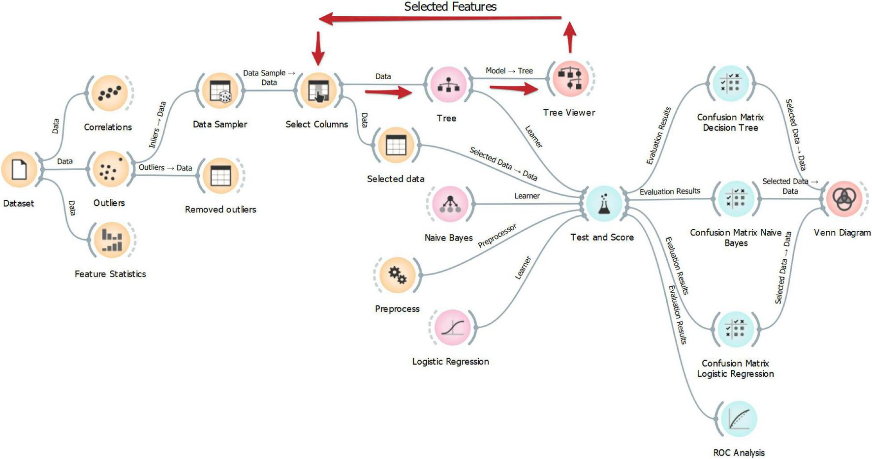
Orange workflow for data analysis.
Performance Measures
By considering PROG class as positive and NON-PROG class as negative, the PROG cases classified as PROG by the classification algorithm were considered true positive (TP); the NON-PROG cases classified as NON-PROG by the classification algorithm were considered true negative (TN); the PROG cases classified as NON-PROG by the classification algorithm were considered false negative (FN); and the NON-PROG cases classified as PROG by the classification algorithm were considered false positive (FP).
The performance of each classification algorithm has been evaluated by computing the AUC of the receiver operating characteristics (ROC) and by computing the following measures: classification accuracy (CA, i.e., the proportion of cases correctly identified by the classification algorithm), precision (i.e., the proportion of TP among cases classified as positive), sensitivity (also indicated as recall, i.e., the proportion of positive cases that are correctly classified), specificity (i.e., the proportion of negative cases that are correctly classified), and F1 (i.e., the weighted harmonic mean of precision and recall).
Statistics and Classification Algorithms Comparison
The Lilliefors test was used to evaluate the hypothesis that each variable had a normal distribution with unspecified mean and variance. Normally distributed variables were presented as mean ± standard deviation (SD); skewed distributed variables were presented as median [interquartile range, IQR]. Differences in mean/median values of variables between the two groups were tested by unpaired Student’s t-test for equal mean and equal but unknown variance or Wilcoxon rank-sum test for equal median.
Comparison of classification algorithms in terms of correctly classified and misclassified cases has been performed by using Venn diagrams. Moreover, comparison of the performance measures (i.e., AUC, CA, precision, sensitivity, specificity, and F1) has been performed by using the Bayesian interpretation of the pairwise Student’s t-tests (Corani and Benavoli, 2015). The statistical significance level was set at 5% for all the tests.
Results
Characteristics of the preprocessed data set are reported in Table 2. With respect to the generated data set given as input to the data analysis procedure, three outliers have been removed (1 NON-PROG and 2 PROG), thus resulting in a total of 75 cases; comparing the characteristics of NON-PROG and PROG, 25 out of 34 characteristics have been found statistically different. Feature selection performed through decision tree provided six features for the classification of PROG vs. NON-PROG, specifically DI, BMI, BSR, age, gb, and CpMEAN; thresholds identified by decision tree were 0.3 min–1, 28.7 kg⋅m–2, 32.4 pmol⋅L−1⋅min−1, 39 years, 95 mg⋅dl−1, and 240 pmol⋅L−1 for DI, BMI, BSR, age, gb, and CpMEAN, respectively (Figure 2). All the selected features have been found to be significantly different between PROG and NON-PROG; however, statistical difference in CpMEAN is not strongly significant (p = 0.04, refer to Table 2).
TABLE 2
| Characteristics | NON-PROG (n = 58) | PROG (n = 17) | p-value |
| age | 33.3 ± 4.2 | 36.6 ± 4.7 | <0.01 |
| BW | 65.8 [15.0] | 75.0 [18.8] | 0.03 |
| h | 164 [12] | 158 [12] | 0.04 |
| BMI | 25.4 ± 3.9 | 30.6 ± 6.4 | <0.001 |
| gb | 84 [8] | 96 [11.50] | <0.001 |
| GMEAN | 5.1 [0.7] | 5.9 [0.8] | <0.001 |
| IMEAN | 201.8 [78.3] | 211.9 [102.8] | n.s. |
| CpMEAN | 182.4 [97.2] | 240.9 [65.4] | 0.04 |
| AUCINS–1P | 2125.5 [1053.2] | 1520.9 [1120.0] | <0.01 |
| AUCINS–2P | 34468.1 [1417.8] | 36992.9 [18872.1] | n.s. |
| KG1 | 1.93 [0.88] | 1.56 [0.63] | <0.001 |
| KG2 | 4.7 ± 1.8 | 3.4 ± 1.8 | 0.01 |
| SI | 4.7 [2.7] | 3.1 [2.0] | 0.02 |
| SG | 0.022 [0.005] | 0.018 [0.008] | <0.01 |
| V | 13.4 [1.36] | 13.9 [1.00] | n.s. |
| BIE | 3 [2.4] | 2.4 [1.5] | n.s. |
| GEZI | 1.9 [0.7] | 1.7 [0.6] | n.s. |
| AIR | 194.4 [126.5] | 132.8 [103.0] | <0.01 |
| ACPR | 254.0 [138.8] | 158.2 [150.0] | <0.01 |
| DI | 1.36 [1.25] | 0.52 [0.76] | <0.001 |
| BSR | 31.8 [10.4] | 39.6 [10.9] | <0.001 |
| Φ1c | 67.80 [31.90] | 42.02 [33.31] | <0.01 |
| AUCSECR | 24734.9 [15607.7] | 32324.0 [11317.6] | 0.03 |
| AUCSECR–1P | 7146.2 [3591.8] | 6252.9 [3285.6] | 0.02 |
| AUCSECR–2P | 17450.7 [15298.7] | 27324.0 [9849.6] | <0.01 |
| CLMEAN | 0.69 [0.42] | 0.78 [0.47] | 0.03 |
| CLMEAN–1P | 3.30 [0.92] | 4.17 [1.76] | n.s. |
| CLMEAN–2P | 0.53 [0.39] | 0.68 [0.35] | <0.01 |
| CLP | 0.39 ± 0.42 | 0.56 ± 0.53 | n.s. |
| FEL | 0.53 [0.14] | 0.50 [0.13] | n.s. |
| IPEAK–FIRST | 53.2 [39.5] | 36.0 [39.3] | <0.01 |
| IPEAK–INJECT | 493 [281] | 559 [150] | n.s. |
| CPEAK | 465 [197] | 380 [140] | 0.04 |
| DOSE | 19.7 [4.5] | 22.5 [5.6] | 0.02 |
Characteristics of the preprocessed data set.
Data are presented as mean ± standard deviation or median [interquartile range]. Significance level: p-values < 0.05. n.s., not significant. Bold values indicate significant differences.
FIGURE 2
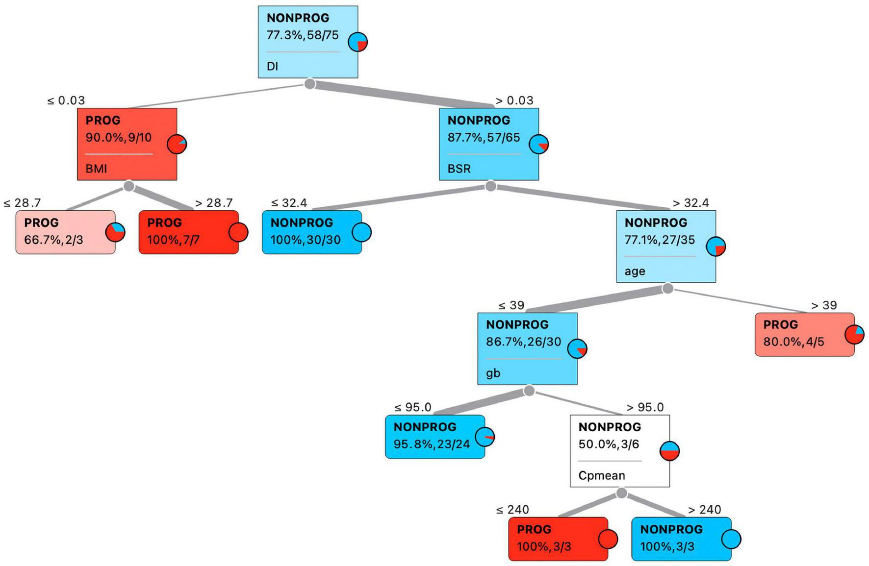
Best predictive features according to decision tree classification algorithm.
Confusion matrices for decision tree, Naïve Bayes, and penalized logistic regression are reported in Figure 3. Correctly classified cases by each classification algorithms were 62, 61, and 63, respectively. The related ROC curves are reported in Figure 4. Results related to the performance of each classification algorithm in terms of AUC, CA, precision, sensitivity, specificity, and F1 are reported in Table 3, and comparison among algorithms are reported in Table 4. Penalized logistic regression outperformed tree and Naïve Bayes in terms of AUC (88.7 vs. 71.7%), CA (57.5 vs. 62.0%), sensitivity (57.5 vs. 62.0%), and F1 (52.8 vs. 54.0%), but not in terms of precision and specificity (in which Naïve Bayes was superior with 64.1 and 86.7%, respectively). The Venn diagrams for comparison among models of correctly classified/misclassified cases are shown in Figure 5; correctly classified or misclassified cases by all the classification algorithms were 53 and 5, respectively.
FIGURE 3
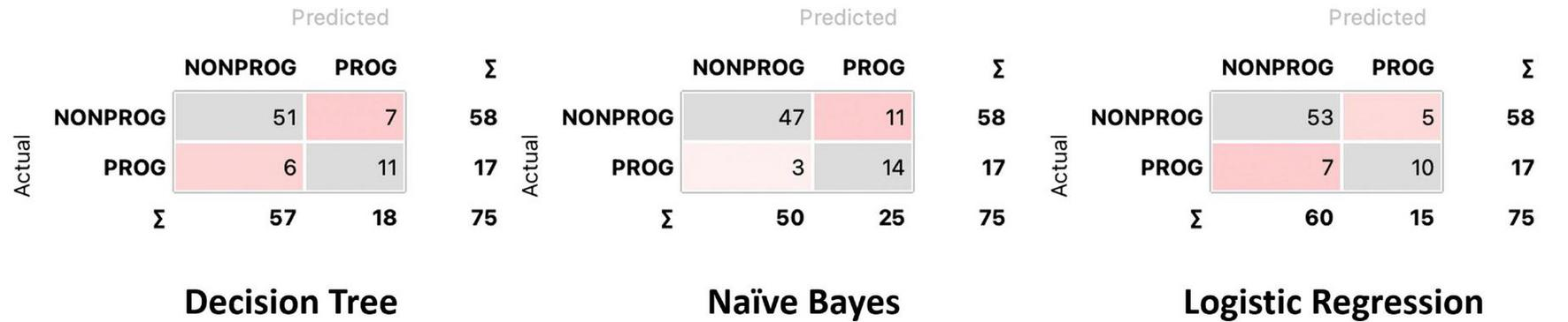
Confusion matrix for decision tree, Naïve Bayes, and logistic regression.
FIGURE 4
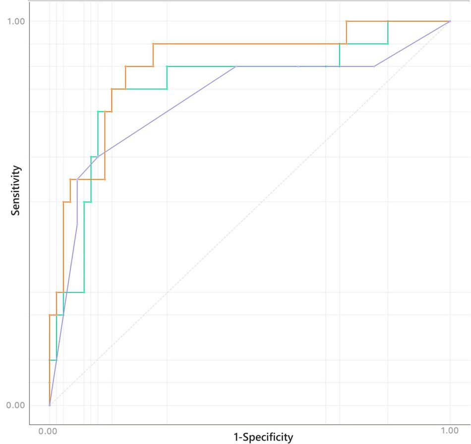
Receiver operating characteristics (ROC) for decision tree (purple), Naïve Bayes (green), and logistic regression (orange).
TABLE 3
| Classification algorithm | |||
| Performance measures | Tree | Naïve Bayes | Logistic regression |
| AUC | 0.795 | 0.831 | 0.884 |
| CA | 0.827 | 0.813 | 0.840 |
| Precision | 0.830 | 0.854 | 0.834 |
| Sensitivity | 0.827 | 0.813 | 0.840 |
| Specificity | 0.700 | 0.821 | 0.662 |
| F1 | 0.828 | 0.824 | 0.836 |
Performance of the three classification algorithms.
TABLE 4
| AUC | |||
| Tree | Naïve Bayes | Logistic regression | |
| Tree | 26.2 | 11.3 | |
| Naïve Bayes | 73.8 | 28.3 | |
| Logistic regression | 88.7 | 71.7 | |
| CA | |||
| Tree | Naïve Bayes | Logistic regression | |
| Tree | 57.5 | 42.5 | |
| Naïve Bayes | 42.5 | 38.0 | |
| Logistic regression | 57.5 | 62.0 | |
| Precision | |||
| Tree | Naïve Bayes | Logistic regression | |
| Tree | 35.9 | 42.0 | |
| Naïve Bayes | 64.1 | 54.0 | |
| Logistic regression | 58.0 | 46.0 | |
| Sensitivity | |||
| Tree | Naïve Bayes | Logistic regression | |
| Tree | 57.5 | 42.5 | |
| Naïve Bayes | 42.5 | 38.0 | |
| Logistic regression | 57.5 | 62.0 | |
| Specificity | |||
| Tree | Naïve Bayes | Logistic regression | |
| Tree | 13.3 | 57.6 | |
| Naïve Bayes | 86.7 | 86.6 | |
| Logistic regression | 42.4 | 13.4 | |
| F1 | |||
| Tree | Naïve Bayes | Logistic regression | |
| Tree | 52.0 | 47.2 | |
| Naïve Bayes | 48.0 | 46.0 | |
| Logistic regression | 52.8 | 54.0 | |
Comparison of the performance measures among classification algorithms through Bayesian interpretation of the pairwise Student’s t-tests.
Probability that the score for the classification algorithm in the row is higher than that of the classification algorithm in the column is reported.
FIGURE 5
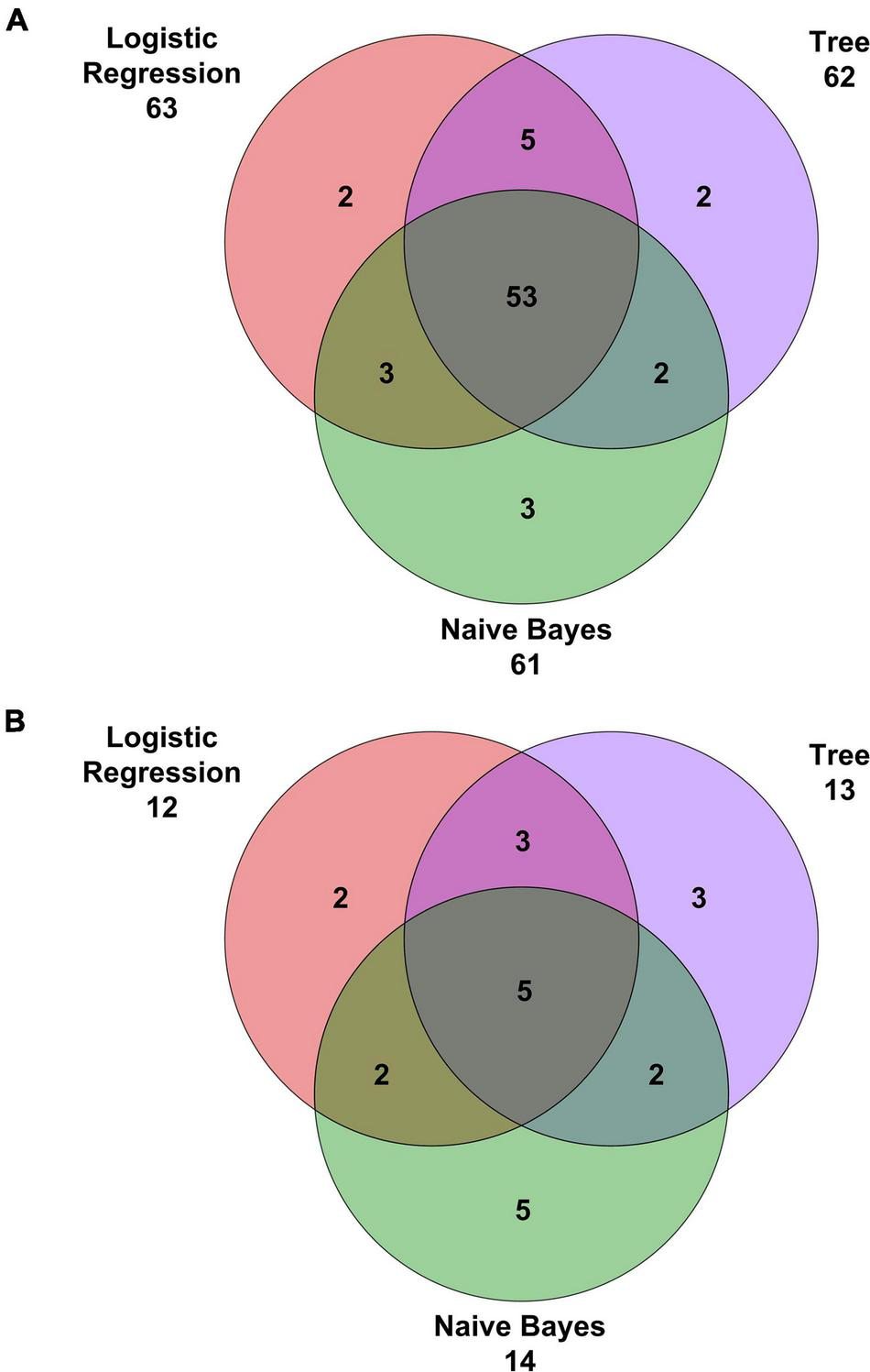
Venn diagrams with (A) correct classifications and (B) misclassifications.
Discussion
This study provided an overview of the most relevant factors that may determine the development of T2DM in women with a history of GDM. Machine-learning techniques were applied to a data set appropriately generated by including features quantifying specific metabolic processes such as insulin sensitivity, β-cell function, and insulin clearance, which are all relevant processes underlying T2DM development (Bizzotto et al., 2021). Inclusion of these features provided a deeper interpretability of the findings, with respect to raw data such as plasma concentrations of glucose, insulin, and C-peptide measured during specific metabolic tests (e.g., IM-IVGTT).
The application of machine-learning techniques to such a kind of database is the main novelty of this study in the context of T2DM risk assessment in women with a history of GDM. In fact, previous studies in the same context have focused on lipidomics or metabolomics (Lappas et al., 2015; Allalou et al., 2016; Khan et al., 2019). In particular, Lappas et al. (2015) aimed to determine whether circulating lipid levels 12 weeks following a pregnancy with GDM were associated with an increased risk of developing T2DM and identified lipid species CE 20:4, PE (P-36:2), and PS 38:4 as significant risk factors. Allalou et al. (2016) and Khan et al. (2019) proposed different predictive signatures, including different metabolites; moreover, reduced sphingolipids have been associated with the pathophysiology of transition from GDM to T2DM (Khan et al., 2019). Since “omics” approaches are still not typically viable in the clinical practice, our study proposed an easier alternative from the technical point of view. In addition, it should be noted that metabolomics/lipidomics predictive power could be enhanced complementing it with classical clinical and biochemical markers (Pallares-Méndez et al., 2016); therefore, our approach could be also used to complement, rather than replace, omics approaches when they will be available in clinical practice.
The main result of this study is the identification of DI, BSR of insulin, and mean area under the C-peptide concentration curve among the most relevant features for the progression to T2DM. DI represents the combined contribution of insulin secretion and insulin sensitivity and was already found to predict conversion to T2DM in a large epidemiological study (Lorenzo et al., 2010); BSR of insulin and mean area under the C-peptide concentration curve are indexes that provide a quantification of insulin secretion. Besides these indexes quantifying specific metabolic processes, age, BMI, and fasting glycemia have been selected.
Three different classification algorithms were tested, namely the decision tree, the Naïve Bayes, and the penalized logistic regression. Comparisons between models were based on AUC, CA, precision, sensitivity, specificity, and F1 and showed that logistic regression resulted the best model for the classification of progression to T2DM since it reported higher values than Naïve Bayes and decision tree in four out of six measures, specifically in AUC, CA, sensitivity, and F1. Naïve Bayes performed better only in precision and specificity, while decision tree reported lower values than the other models in all the measures. Moreover, logistic regression presented higher value of correct classification and lower value of misclassification, followed by decision tree and Naïve Bayes. Moreover, regularized regression methods (L1 or L2, as in this study) are characterized by including a small bias into the maximum likelihood estimation; the inclusion of this bias helps to reduce the variance, thus improving the predictions for new subjects (or the generalization of results) (Hastie, 2017).
Machine-learning techniques have been extensively explored in recent years for the prevention and management of T2DM (Huang et al., 2007; Yu et al., 2010; Perveen et al., 2016; Dalakleidi et al., 2017; Maniruzzaman et al., 2017; Zheng and Zhang, 2017; Talaei-Khoei and Wilson, 2018; Bernardini et al., 2019, 2020) but also showing possible criticalities. In fact, very often, the analysis with these techniques on large amounts of heterogeneous data leads to identify spurious correlations (Rumbold et al., 2020), indicating that the creation of appropriate databases, with selected groups of subjects and characteristics, as done in this study, is an aspect of primary importance and which cannot be disregarded in order to achieve reliable results. Thus, even though the considered population of women with a history of GDM was constituted by a limited number of subjects, they have been strictly controlled and monitored during a long follow-up. Moreover, the subjects have been carefully screened to detect outliers, and these were dropped out from the data set before the analysis; decision of dropping out the outliers instead of performing data imputation only for specific features was taken to reduce as much as possible bias and uncertainty. Adoption of machine-learning techniques, usually devoted to the analysis of large amounts of data, is justified in this study by the high number of features included in the generated data set, from which such techniques may allow determination of the most relevant ones. At the same time, when considering a low number of subjects with a high number of features, overfitting may occur and achieved results may be a bit optimistic, especially when using decision tree algorithm. It has to be acknowledged that this may be the risk of this study. However, well-known strategies have been adopted to mitigate this risk, namely, pruning (through which the redundant branches can be cut beforehand) and k-fold cross-validation (Zhou et al., 2021).
In this study, data analysis has been performed by using Orange (Demšar et al., 2013), an open-source data visualization, machine learning, and data mining toolkit. This software has the advantage of providing a visual programming front-end for explorative rapid qualitative data analysis and interactive data visualization; on the other side, possibilities in data analysis are limited by the procedures implemented in the Orange “building blocks.” Further studies may explore different and more customizable learning algorithms starting from the results of this study.
Conclusion
This study was the first to apply machine-learning techniques to databases that contain features quantifying metabolic processes based on such standard clinical test in women with a history of GDM and at risk of developing T2DM. We found that DI, BSR of insulin, mean area under the C-peptide concentration curve, age, BMI, and fasting glycemia were identified as the most relevant features for the progression from GDM to T2DM. The obtained information from this pattern could be of interest for the study and characterization of diabetes pathophysiology.
Publisher’s Note
All claims expressed in this article are solely those of the authors and do not necessarily represent those of their affiliated organizations, or those of the publisher, the editors and the reviewers. Any product that may be evaluated in this article, or claim that may be made by its manufacturer, is not guaranteed or endorsed by the publisher.
Statements
Data availability statement
The data analyzed in this study is subject to the following licenses/restrictions: The datasets generated and/or analyzed in the current study are available from AK-W on reasonable request. Requests to access these datasets should be directed to AK-W, alexandra.kautzky-willer@meduniwien.ac.at.
Ethics statement
The studies involving human participants were reviewed and approved by the Ethics Committee of the Medical University of Vienna. The patients/participants provided their written informed consent to participate in this study.
Author contributions
LI, AP, AT, and MM contributed to conception and design of the study. CG and AK-W contributed to acquisition of data. LI, AP, CG, LB, AK-W, AT, and MM analyzed and interpreted the data. LI, AT, and MM drafted the article. AP, CG, LB, and AK-W revised the article. All authors have read and approved the submitted version of the article.
Conflict of interest
The authors declare that the research was conducted in the absence of any commercial or financial relationships that could be construed as a potential conflict of interest.
Footnotes
References
1
AllalouA.NallaA.PrenticeK. J.LiuY.ZhangM.DaiF. F.et al (2016). A predictive metabolic signature for the transition from gestational diabetes mellitus to type 2 diabetes.Diabetes652529–2539. 10.2337/db15-1720
2
American Diabetes Association (2020). 2. Classification and diagnosis of diabetes: standards of medical care in diabetes-2020.Diabetes Care43S14–S31. 10.2337/dc20-S002
3
BernardiniM.MorettiniM.RomeoL.FrontoniE.BurattiniL. (2019). TyG-er: an ensemble regression forest approach for identification of clinical factors related to insulin resistance condition using electronic health records.Comput. Biol. Med.112:103358. 10.1016/j.compbiomed.2019.103358
4
BernardiniM.MorettiniM.RomeoL.FrontoniE.BurattiniL. (2020). Early temporal prediction of type 2 diabetes risk condition from a general practitioner electronic health record: a multiple instance boosting approach.Artif. Intell. Med.105:101847. 10.1016/j.artmed.2020.101847
5
BizzottoR.JennisonC.JonesA. G.KurbasicA.TuraA.KennedyG.et al (2021). Processes underlying glycemic deterioration in type 2 diabetes: an IMI DIRECT study.Diabetes Care44511–518. 10.2337/dc20-1567
6
BreuniqM. M.KriegelH. P.NgR. T.SanderJ. (2000). LOF: identifying density-based local outliers.SIGMOD Rec.2993–104. 10.1145/335191.335388
7
CoraniG.BenavoliA. (2015). A bayesian approach for comparing cross-validated algorithms on multiple data sets.Mach. Learn.100285–304. 10.1007/s10994-015-5486-z
8
DalakleidiK.ZarkogianniK.ThanopoulouA.NikitaK. (2017). Comparative assessment of statistical and machine learning techniques towards estimating the risk of developing type 2 diabetes and cardiovascular complications.Expert Syst.34:e12214. 10.1111/exsy.12214
9
DemšarJ.CurkT.ErjavecA.GorupČHočevarT.MilutinovičM.et al (2013). Orange: data mining toolbox in python.J. Mach. Learn. Res.142349–2353.
10
El_JerjawiN. S.Abu-NaserS. S. (2018). Diabetes prediction using artificial neural network.Int. J. Adv. Sci. Technol.12154–64.
11
Garcia-CarreteroR.Vigil-MedinaL.Barquero-PerezO. (2021). The use of machine learning techniques to determine the predictive value of inflammatory biomarkers in the development of type 2 diabetes mellitus.Metab. Syndr. Relat. Disord.19240–248. 10.1089/met.2020.0139
12
Garcia-CarreteroR.Vigil-MedinaL.Mora-JimenezI.Soguero-RuizC.Barquero-PerezO.Ramos-LopezJ. (2020). Use of a K-nearest neighbors model to predict the development of type 2 diabetes within 2 years in an obese, hypertensive population.Med. Biol. Eng. Comput.58991–1002. 10.1007/s11517-020-02132-w
13
GöblC. S.BozkurtL.TuraA.PaciniG.Kautzky-WillerA.MittlböckM. (2015). Application of penalized regression techniques in modelling insulin sensitivity by correlated metabolic parameters.PLoS One10:e0141524. 10.1371/journal.pone.0141524
14
HastieT. T. (2017). The elements of statistical learning, Second Edn. Berlin: Springer.
15
HuangY.McCullaghP.BlackN.HarperR. (2007). Feature selection and classification model construction on type 2 diabetic patients’ data.Artif. Intell. Med.41251–262. 10.1016/j.artmed.2007.07.002
16
JohnstonC.RaghuP.McCullochD. K.BeardJ. C.WardW. K.KlaffL. J.et al (1987). Beta-cell function and insulin sensitivity in nondiabetic HLA-identical siblings of insulin-dependent diabetics.Diabetes36829–837. 10.2337/diab.36.7.829
17
KahnS. E.KlaffL. J.SchwartzM. W.BeardJ. C.BergmanR. N.TaborskyG. J.et al (1990). Treatment with a somatostatin analog decreases pancreatic B-cell and whole body sensitivity to glucose.J. Clin. Endocrinol. Metab.71994–1002. 10.1210/jcem-71-4-994
18
KahnS. E.PrigeonR. L.McCullochD. K.BoykoE. J.BergmanR. N.SchwartzM. W.et al (1993). Quantification of the relationship between insulin sensitivity and -cell function in human subjects: evidence for a hyperbolic function.Diabetes421663–1672. 10.2337/diab.42.11.1663
19
KavakiotisI.TsaveO.SalifoglouA.MaglaverasN.VlahavasI.ChouvardaI. (2017). Machine learning and data mining methods in diabetes research.Comput. Struct. Biotechnol. J.15104–116. 10.1016/j.csbj.2016.12.005
20
KhanS. R.MohanH.LiuY.BatchuluunB.GohilH.Al RijjalD.et al (2019). The discovery of novel predictive biomarkers and early-stage pathophysiology for the transition from gestational diabetes to type 2 diabetes.Diabetologia62687–703. 10.1007/s00125-018-4800-2
21
KlassenA.FaccioA. T.CanutoG. A. B.da CruzP. L. R.RibeiroH. C.TavaresM. F. M.et al (2017). Metabolomics: definitions and significance in systems biology.Adv. Exp. Med. Biol.9653–17. 10.1007/978-3-319-47656-8_1
22
LappasM.MundraP. A.WongG.HuynhK.JinksD.GeorgiouH. M.et al (2015). The prediction of type 2 diabetes in women with previous gestational diabetes mellitus using lipidomics.Diabetologia581436–1442. 10.1007/s00125-015-3587-7
23
LorenzoC.WagenknechtL. E.RewersM. J.KarterA. J.BergmanR. N.HanleyA. J. G.et al (2010). Disposition index, glucose effectiveness, and conversion to type 2 diabetes: the Insulin Resistance Atherosclerosis Study (IRAS).Diabetes Care332098–2103. 10.2337/dc10-0165
24
ManiruzzamanM.KumarN.Menhazul AbedinM.Shaykhul IslamM.SuriH. S.El-BazA. S.et al (2017). Comparative approaches for classification of diabetes mellitus data: machine learning paradigm.Comput. Methods Programs Biomed.15223–34. 10.1016/j.cmpb.2017.09.004
25
MariA.TuraA.GrespanE.BizzottoR. (2020). Mathematical modeling for the physiological and clinical investigation of glucose homeostasis and diabetes.Front. Physiol.11:575789. 10.3389/fphys.2020.575789
26
MorettiniM.CastriotaC.GöblC.Kautzky-WillerA.PaciniG.BurattiniL.et al (2020a). Glucose effectiveness from short insulin-modified IVGTT and its application to the study of women with previous gestational diabetes mellitus.Diabetes Metab. J.44286–294. 10.4093/dmj.2019.0016
27
MorettiniM.GöblC.Kautzky-WillerA.PaciniG.TuraA.BurattiniL. (2020b). Former gestational diabetes: mathematical modeling of intravenous glucose tolerance test for the assessment of insulin clearance and its determinants.Math. Biosci. Eng.171604–1615. 10.3934/mbe.2020084
28
PaciniG.TonoloG.SambataroM.MaioliM.CiccareseM.BroccoE.et al (1998). Insulin sensitivity and glucose effectiveness: minimal model analysis of regular and insulin-modified FSIGT.Am. J. Physiol. Metab.274E592–E599. 10.1152/ajpendo.1998.274.4.e592
29
Pallares-MéndezR.Aguilar-SalinasC. A.Cruz-BautistaI.Del Bosque-PlataL. (2016). Metabolomics in diabetes, a review.Ann. Med.4889–102. 10.3109/07853890.2015.1137630
30
PerveenS.ShahbazM.GuergachiA.KeshavjeeK. (2016). Performance analysis of data mining classification techniques to predict diabetes.Procedia Comput. Sci.82115–121. 10.1016/j.procs.2016.04.016
31
PinuF. R.GoldansazS. A.JaineJ. (2019). Translational metabolomics: current challenges and future opportunities.Metabolites9:108. 10.3390/metabo9060108
32
PlowsJ. F.StanleyJ. L.BakerP. N.ReynoldsC. M.VickersM. H. (2018). The pathophysiology of gestational diabetes mellitus.Int. J. Mol. Sci.19:3342. 10.3390/ijms19113342
33
PolidoriD. C.BergmanR. N.ChungS. T.SumnerA. E. (2016). Hepatic and extrahepatic insulin clearance are differentially regulated: results from a novel model-based analysis of intravenous glucose tolerance data.Diabetes651556–1564. 10.2337/db15-1373
34
RumboldJ. M. M.O’KaneM.PhilipN.PierscionekB. K. (2020). Big data and diabetes: the applications of big data for diabetes care now and in the future.Diabet. Med.37187–193. 10.1111/dme.14044
35
SarwarM. A.KamalN.HamidW.ShahM. A. (2018). “Prediction of diabetes using machine learning algorithms in healthcare,” in ICAC 2018 - 2018 24th IEEE International Conference on Automation and Computing: Improving Productivity through Automation and Computing.10.23919/IConAC.2018.8748992
36
Talaei-KhoeiA.WilsonJ. M. (2018). Identifying people at risk of developing type 2 diabetes: a comparison of predictive analytics techniques and predictor variables.Int. J. Med. Inform.11922–38. 10.1016/j.ijmedinf.2018.08.008
37
TuraA.GöblC.MorettiniM.BurattiniL.Kautzky-WillerA.PaciniG. (2020). Insulin clearance is altered in women with a history of gestational diabetes progressing to type 2 diabetes.Nutr. Metab. Cardiovasc. Dis.301272–1280. 10.1016/j.numecd.2020.04.004
38
TuraA.GrassiA.WinhoferY.GuoloA.PaciniG.MariA.et al (2012). Progression to type 2 diabetes in women with former gestational diabetes: time trajectories of metabolic parameters.PLoS One.7:e50419. 10.1371/journal.pone.0050419
39
Van CauterE.MestrezF.SturisJ.PolonskyK. S. (1992). Estimation of insulin secretion rates from C-peptide levels. Comparison of individual and standard kinetic parameters for C-peptide clearance.Diabetes41368–377.
40
YuW.LiuT.ValdezR.GwinnM.KhouryM. J. (2010). Application of support vector machine modeling for prediction of common diseases: the case of diabetes and pre-diabetes.BMC Med. Inform. Decis. Mak.10:16. 10.1186/1472-6947-10-16
41
ZhengT.ZhangY. (2017). “A big data application of machine learning-based framework to identify type 2 diabetes through electronic health records,” in Knowledge Management in Organizations. KMO 2017. Communications in Computer and Information Science, Vol. 731, edsUdenL.LuW.TingI. H. (Cham:Springer). 10.1007/978-3-319-62698-7_37
42
ZhouH. F.ZhangJ. W.ZhouY. Q.GuoX. J.MaY. M. (2021). A feature selection algorithm of decision tree based on feature weight.Expert Syst. Appl.164:113842. 10.1016/J.ESWA.2020.113842
43
ZouQ.QuK.LuoY.YinD.JuY.TangH. (2018). Predicting diabetes mellitus with machine learning techniques.Front. Genet.9:515. 10.3389/fgene.2018.00515
Summary
Keywords
pathophysiology, predictive biomarker, disease prediction, statistical learning, logistic regression, mathematical model
Citation
Ilari L, Piersanti A, Göbl C, Burattini L, Kautzky-Willer A, Tura A and Morettini M (2022) Unraveling the Factors Determining Development of Type 2 Diabetes in Women With a History of Gestational Diabetes Mellitus Through Machine-Learning Techniques. Front. Physiol. 13:789219. doi: 10.3389/fphys.2022.789219
Received
04 October 2021
Accepted
11 January 2022
Published
17 February 2022
Volume
13 - 2022
Edited by
Matteo Barberis, University of Surrey, United Kingdom
Reviewed by
Óscar Barquero-Pérez, Rey Juan Carlos University, Spain; Ying Sun, Xuzhou Medical University, China
Updates
Copyright
© 2022 Ilari, Piersanti, Göbl, Burattini, Kautzky-Willer, Tura and Morettini.
This is an open-access article distributed under the terms of the Creative Commons Attribution License (CC BY). The use, distribution or reproduction in other forums is permitted, provided the original author(s) and the copyright owner(s) are credited and that the original publication in this journal is cited, in accordance with accepted academic practice. No use, distribution or reproduction is permitted which does not comply with these terms.
*Correspondence: Micaela Morettini, m.morettini@univpm.it
This article was submitted to Computational Physiology and Medicine, a section of the journal Frontiers in Physiology
Disclaimer
All claims expressed in this article are solely those of the authors and do not necessarily represent those of their affiliated organizations, or those of the publisher, the editors and the reviewers. Any product that may be evaluated in this article or claim that may be made by its manufacturer is not guaranteed or endorsed by the publisher.