Automated depth correction of bathymetric LiDAR point clouds using PointCNN semantic segmentation

The study explores deep learning to perform direct semantic segmentation of bathymetric lidar points to improve bathymetry mapping. Focusing on river bathymetry, the goal is to accurately and simultaneously classify points on the benthic layer, water surface, and ground near riverbanks. These classifications are then used to apply depth correction to all points within the water column. The study aimed to classify the scene into four classes: river surface, riverbed, ground, and other (for points outside of those three classes), focusing on the river surface and riverbed classes. To achieve this, PointCNN, a convolutional neural network model adept at handling unorganized and unstructured data in 3D space was implemented. The model was trained with airborne bathymetric lidar data from the Swan River in Montana and the Eel River in California. The model was tested on the Snake River in Wyoming to evaluate its performance. These diverse bathymetric datasets across the United States provided a solid foundation for the model’s robust testing. The results were strong for river surface classification, achieving an Intersection over Union of (0.89) and a Kappa coefficient of (0.92), indicating high reliability and minimal errors. The riverbed classification also showed an IoU of (0.7) and a slightly higher Kappa score of (0.76). Depth correction was then performed on riverbed points, proportional to the calculated depth from a surface model formed by Delaunay triangulation of ground and river surface points. The automated process performs significantly faster than traditional manual classification and depth correction processes, saving time and expense. Finally, corrected depths were quantitatively validated by comparing with independent Acoustic Doppler Current Profiler measurements from the Snake River, obtaining a mean depth error of 2 cm and an Root mean square error of 16 cm. These validation results show the reliability and accuracy of the proposed automated bathymetric depth correction workflow.

1 Introduction

Lidar systems produce 3D point clouds, providing high-resolution data essential for geoscientists to analyze natural and artificial features. These clouds consist of millions of individual points, each with x, y, and z coordinates and possibly other features like intensity and RGB; collectively forming a comprehensive 3D model of the surveyed area. Aerial bathymetric lidar systems are designed to map underwater features using laser pulses that can penetrate water, normally operating at a wavelength of $\lambda =532\text{\hspace{0.17em}nm}$ (green). Bathymetric lidar sensors provide high-resolution data of submerged environments, precisely documenting shallow underwater terrain (Pan et al., 2015a). An accurate digital model of the benthic layer is crucial for mapping habitats in fluvial and coastal areas (Letard et al., 2022), enhancing flood inundation models (Teng et al., 2015), tracking sediment transport (Anderson and Pitlick, 2014), and for nearshore bathymetry (Albright and Glennie, 2021). It is invaluable for coastal management to monitor erosion, identify submerged hazards (Pricope and Bashit, 2023), guide infrastructure planning, and conserve ecosystems like coral reefs and seagrasses (Wilson, 2011; Pan et al., 2014).

Processing bathymetric lidar data has significant challenges, primarily due to the refraction of the laser pulses in water. While shifts in the $x$ and $y$ coordinates are minor and dependent upon the scan angle, the $z$ coordinate (elevation) shifts are more pronounced. This is because water, with a nominal refractive index of approximately 1.33 (Xiao et al., 2024), bends and slows the light, distorting true depths because the travel time of the laser pulses in water is unknown without precise knowledge of both the water surface and benthic layer locations (Agrafiotis et al., 2019; Schwarz et al., 2021). Fluvial environments face significant challenges due to fluctuating water elevations along a river’s course, especially downstream, where levels can drop rapidly (Mandlburger et al., 2015). Dams exacerbate this, causing abrupt elevation changes that complicate water surface point detection and classification (Letard et al., 2024). Rivers often have complex hydrological structures with multiple braided channels that diverge and rejoin, connecting with abandoned channels or adjacent floodplain lakes, adding to the complexity. The Snake River in Wyoming, United States, as shown in Figure 1, exemplifies these challenges.

Figure 1

Figure 1. Snake River, Wyoming, in (a) a dam, and (b) shows a braided river channel, which contributes to the complexity of the river system due to varying flow dynamics, sediment transport, and multiple interconnecting channels.

The industry standard to correct unknown travel time in water involves manually classifying the water surface and water column points using a filtering method, creating two surface model using benthic and water surface points separately, calculating the depth of water column and waterbed points, and finally correcting their elevation proportionate to their depth based on the travel time in water and the resulting change in the speed of light. For the same Snake River dataset, previous studies such as Legleiter et al. (2016) applied an adaptive TIN filter (Axelsson, 2000) to identify candidate water surface points, followed by manual editing to refine surface and bottom separation. A channel centerline was then fitted to the surface points, and refraction correction was applied to bottom returns using the time difference between green laser surface and benthic echoes. Two separate surface models were generated for the water surface and riverbed, and morphological filtering was used to remove noise. Pan et al. (2015a) used a continuous wavelet transform to pick seed peaks in each full waveform, then manually classified those peaks into water surface, water-column, and benthic returns and corrected their ranges using the refractive index. The manual process of refraction and depth correction for bathymetric lidar data is inherently time-consuming and susceptible to human error due to the repetitive nature of the tasks. Therefore, developing an automated methodology to ensure precision, efficiency, and repeatability is needed. Automating these corrections can significantly reduce processing time and minimize the introduction of errors, thereby improving the reliability of bathymetric measurements.

Current machine learning research using bathymetric airborne laser scanning (ALS) focuses on detecting structures (Tsai et al., 2021), and identifying vegetation. Daniel and Dupont (2020) used a convolutional neural network (CNN) for seabed features, and Erena et al. (2019) highlight drones for high-resolution topo-bathymetric monitoring. While shallow water applications are well-documented (Wang and Philpot, 2007; Hyejin Kim et al., 2023), deep learning for water-level semantic segmentation is limited. Innovative methods like pseudo-waveform decomposition (Hyejin Kim et al., 2023) and multispectral imaging (Mandlburger et al., 2021) exist, but purely point cloud applications remain largely unexplored, indicating a need for further research. Bouhdaoui et al. (2014) studied the impact of complex water bottom geometries on peak time shifting in bathymetric lidar waveforms, using the Wa-LID waveform simulator to model different depths, slopes, and footprint sizes. Zhou et al. (2023) addressed water depth bias correction by subdividing the water area into sub-regions based on water depths and biases, using a subdivision algorithm and least-squares regression. Agrafiotis et al. (2019) applied a support vector regression (SVR) model to correct depth underestimation in point clouds from structure from motion (SfM) and multi-view stereo (MVS) techniques, using known depth data from bathymetric lidar to enhance accuracy and robustness by fusing the lidar and image-based point clouds. For aerial bathymetric lidar data alone, semantic segmentation is crucial yet underexplored for segmenting river surfaces using deep learning.

Recent advances in 3D point cloud segmentation have led to a wide range of deep learning models categorized by their core processing methods. Pointwise MLP-based models such as PointNet (Qi et al., 2016) and PointNet++ (Qi et al., 2017) learn per-point features using shared multilayer perceptrons and aggregate them with symmetric functions. RandLA-Net (Hu et al., 2020) and ShellNet (Zhang et al., 2019) improve efficiency and local structure learning, though MLP-based methods generally lack strong spatial context modeling. Volumetric methods, such as SEGCloud (Tchapmi et al., 2017) and SparseConvNet (Graham et al., 2018), convert point clouds into voxel grids before processing, which allows the use of 3D convolutions but sacrifices geometric precision and incurs high memory and computation due to voxelization. These methods do not operate directly on the raw point cloud and may lose fine-grained details. Spherical projection models such as SqueezeSeg (Wu et al., 2018) transform 3D data into 2D spherical range images to enable fast processing with 2D convolutions. However, this transformation alters the spatial structure and introduces distortions, limiting the model’s ability to preserve the native geometry of the point cloud. Point convolution methods and graph-based methods represent the most reliable classes of architectures. PointCNN (Li et al., 2018) and DGCNN (Wang et al., 2019b) are widely recognized as the standard baselines in these categories due to their consistent performance. PointCNN transforms unordered inputs into canonical forms for convolution, while models like PCNN (Atzmon et al., 2018), ConvPoint (Boulch, 2020), and KPConv (Thomas et al., 2019) apply continuous or deformable filters. Graph-based models such as DGCNN and GACNet (Wang et al., 2019a) dynamically build neighborhood graphs and extract features using edge-based mechanisms. According to Bello et al. (2020), many deep learning models for point cloud segmentation achieve comparable performance across standard benchmarks. Therefore, we focus on PointCNN and DGCNN, which are inherently different in design but have been widely used across diverse applications and reflect the two dominant paradigms of point cloud learning (Lumban-Gaol et al., 2021; Koguciuk et al., 2019).

3D semantic segmentation is widely applied in computer vision and remote sensing, providing point-wise segmentation of point clouds. In environmental applications, topographic and bathymetric lidar data are used for land cover mapping (Arief et al., 2018; Ekhtari et al., 2018; Zhang et al., 2022), distinguishing terrestrial and aquatic features to support hydrological modeling, flood risk analysis, and environmental monitoring (Zhao et al., 2016). Building on segmentation methods, PointCNN (Li et al., 2018) and DGCNN (Wang et al., 2019b) represent two leading architectures for 3D point cloud processing. PointCNN, adapted from PointNet++ (Qi et al., 2017), introduces hierarchical feature learning and has been applied in environmental mapping (Fareed et al., 2023), 3D object recognition (Koguciuk et al., 2019), and autonomous navigation (A Arief et al., 2019). DGCNN extends PointNet (Qi et al., 2016) with dynamic graph-based convolutions to better capture local and global shape information. These models are not only technically robust but also highly relevant in practical domains, establishing themselves as essential tools for modern 3D data understanding.

Achieving accurate segmentation of bathymetric lidar through deep learning models like PointCNN or DGCNN can eliminate the need for manual processes, which are time-consuming and prone to human error due to their qualitative and repetitive nature. Manual classification lacks repeatability, as two individuals performing the classification independently may get different results. Utilizing deep learning models can streamline the workflow by removing the necessity for additional steps such as delineating the river, incorporating external images for verification, and manually classifying the water surface. This new automated approach enhances efficiency, accuracy and repeatability in the classification of bathymetric lidar data by performing water column classification with high precision. Although PointCNN and DGCNN presented as candidate segmentation approaches in this study, the workflow remains architecture-agnostic; any point-cloud network (e.g., PointNet++, KPConv, or a transformer-based model) capable of reliably separating water-surface from water-bed points can be substituted without altering the subsequent refraction-correction and depth-estimation steps. To our knowledge, this is the first model trained and tested for simultaneous semantic segmentation for both the river surface and riverbed. The segmentation of these two layers aids in the calculation of water depth, making it more automated and accurate for refraction and depth correction of the benthic layer.

2 Study area and methods

2.1 Study area

The three datasets used in this study, shown in Table 1, are bathymetric lidar survey data for three rivers in the United States: the Swan River in Montana, the Snake River in Wyoming, and the Eel River in California. All three datasets were collected by the National Center for Airborne Laser Mapping (NCALM) (ncalm.cive.uh.edu) and the data includes independent ground truth data. The ground truth was created using manual classification, ensuring high accuracy through multiple iterations. The process involved using Terrasolid’s Terrascan software to guarantee precise data labeling, with verification using Google Earth images. The Swan River survey was conducted in 2023, the Snake River in 2012, and the Eel River in 2014. These surveys cover a range of geographical areas, with the Swan River encompassing 53 ${\text{km}}^2$, the Snake River 77 ${\text{km}}^2$, and the Eel River 57 ${\text{km}}^2$. However, only a narrow corridor along each river was selected for analysis to focus the study on only the river itself, significantly reducing the total point count and concentrating solely on river classes as shown in Table 2. The surveyed corridor length of these rivers is 27 km for the Swan River, 44 km for the Snake River, and 204 km for the Eel River. An important aspect of these surveys is the point density, expressed as the number of lidar points per square meter. This metric is used for determining the survey data’s resolution and level of detail. The Swan River survey has a high point density of 28 ${\text{pts/m}}^2$, which suggests a very detailed and fine-scale survey. In contrast, the Snake River survey has a much lower point density of 3 ${\text{pts/m}}^2$, indicating a coarser resolution. The Eel River survey falls between these two, with a point density of 14 ${\text{pts/m}}^2$. The sensor technologies employed for these surveys also differ, reflecting technological advancements and specific sensor capabilities. The Snake River and Eel River surveys were conducted using the Optech AQUARIUS sensor (Guo et al., 2018) and the Swan River survey used the RIEGL VQ-840-G sensor (Pfennigbauer et al., 2022). The datasets used in our study are diverse in terms of river hydrogeomorphology, lidar sensor technologies, and point cloud densities. This diversity enhances the robustness and generalizability of any machine learning model, allowing it to effectively learn and predict river channel evolution in various geographic and environmental contexts.

Table 1

Table 1. Details of lidar datasets used in this research.

Table 2

Table 2. Total points after clipping to river center corridor and class percentage distribution for each river dataset.

The data for all three rivers were manually classified into four categories: river surface, riverbed, ground, and other. The river surface class represents the interface between the water and the atmosphere, capturing the mostly specular reflection of laser light on the water surface. The riverbed class encompasses the benthic layer at the bottom of the water, including both the sediment and any submerged vegetation. The riverbed class also accounts for volumetric scattering in the water column. Volumetric scattering occurs when light interacts with suspended particles and water molecules. These interactions cause the lidar signal to scatter in multiple directions, affecting its penetration depth and the peak of the backscatter signal received. The ground class includes terrestrial surfaces, excluding aquatic or vegetative components, clearly differentiated from the marine environment. Lastly, the other class includes all remaining data points that do not fall into the previous three categories and predominantly consist of vegetation. This categorization ensures comprehensive mapping and analysis of the riverine and adjacent environments. To focus on the riverine environment, only a subset of each dataset was used, including points along a 50-m corridor from the centerline of each river. The class distribution for this corridor is given in Table 2. Even after reducing to a narrow along the river, the ground and other classes still comprise the majority of points, whereas the river surface and riverbed classes account for only a small percentage.

To validate our depth corrections on the Snake River, we used the ground truth acquired by Legleiter et al. (2016). They surveyed Rusty Bend (a specific bend in the Snake River) with a SonTek RiverSurveyor S5 Acoustic Doppler Current Profiler (ADCP) mounted on a kayak and tied to an RTK-GPS base station, getting depth soundings with 0.001 m resolution and 1% accuracy over 0.2–15 m. Along the channel margins, they also measured water edge elevations with RTK-GPS to correct for instrument drift and kayak offset. All ADCP returns within 0.5 m of a GPS control point were cross-calibrated to ensure vertical consistency. We used these rigorously corrected and georeferenced ADCP measurements as the bathymetric ground-truth along the Snake River for validating our fully automated depth correction model.

2.2 Methodology

The methodology starts with the data processing steps used to convert light detection and ranging files into uniformly sized blocks suitable for deep learning input. The process continues with data augmentation techniques aimed at increasing the dataset’s size and generalizability for the machine learning model. The model is then discussed with an in-depth analysis of the PointCNN implementation using ESRI’s deep learning module arcgis.learn (Esri, 2024). Different metrics and error rates are then used to evaluate the model’s performance. Finally, the methodology addresses depth and refraction corrections to achieve the desired corrected final riverbed points, as shown in Figure 2.

Figure 2

Figure 2. Workflow diagram showing the steps involved in this research. The process starts with input data, followed by pre-processed data where data cleaning and transformation occur. Augmenting the dataset is the next step in enhancing the training dataset. After the training and testing phase, the model is evaluated against the ground truth. Finally, depth and refraction corrections are applied to the riverbed points classified by the model.

2.2.1 Data preprocessing

Point cloud data cannot be directly fed into a deep learning model due to its unstructured and unorganized nature. To make it suitable for deep learning, the data must be preprocessed into a uniform dataset, as demonstrated in methods such as, Pointnet++ (Qi et al., 2017) and PointCNN (Li et al., 2018). The entire dataset is broken down into smaller blocks, each with a constant size of $S$ x $S$ as shown in Figure 3. Block size $S$ is selected based on the specific application requirements as determined by the user. Block sizes are based on the data characteristics, scene complexity, and point density.

Figure 3

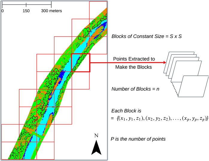
Figure 3. Point cloud data (with ground truth) is divided into frames, as seen on the left side of the diagram. Points are extracted from each frame to create uniform-sized blocks $S$ x $\mathrm{S}$ (square blocks are required for the model) with a fixed number of points $P$ using Farthest Point Sampling (FPS). $n$ number of blocks are generated after a single frame is fully sampled.

The gridded squares shown in Figure 3 are the frames that contain the raw point cloud sets. Points are sampled from these frames to create the final product called a block. The sampling from each frame starts with an initial point selected randomly. This point serves as the starting reference for the sampling process. Because the initial point is chosen randomly, it introduces some variability in the sampling process; different initial points can lead to different sampled sets. From this initial point, Farthest Point Sampling (FPS) (Qi et al., 2017) calculates the Euclidean distance to every other point in the point cloud frame. The point farthest from this initial point, i.e., the point with the maximum distance, is then selected and added to the sampled set. In subsequent iterations, the algorithm updates the newly added point as the reference to find the next farthest point. This iterative process continues until the desired number of points are chosen and a block is created. Each block is represented as a set of points:

$\left\{\left(x_1,y_1,z_1\right),\left(x_2,y_2,z_2\right),\dots ,\left(x_p,y_p,z_p\right)\right\}$

where $P$ is the number of points within the block. Similar to block size, the value of $P$ can be decided based on point density, however, another critical factor is computational power. The larger the value of $P$, the more dedicated memory is required. Once the sample set is complete, the process repeats on the remaining points in the frame until all points are sampled to create blocks. FPS effectively spreads out the sampled points, ensuring a uniform and comprehensive coverage of the entire point cloud. This method preserves the structural diversity and spatial distribution of the original dataset.

2.2.2 Augmenting data

A rotation matrix about the z-axis is extensively used to augment point cloud data in various machine learning and computer vision applications (Shi et al., 2021; Choi et al., 2021). This matrix, given by:

$R_z\left(\theta \right)=\left[\begin{array}{ccc}\hfill \cos \theta \hfill & \hfill -\sin \theta \hfill & \hfill 0\hfill \\ \hfill \sin \theta \hfill & \hfill \cos \theta \hfill & \hfill 0\hfill \\ \hfill 0\hfill & \hfill 0\hfill & \hfill 1\hfill \end{array}\right],$

allows for the rotation of 3D points around the z-axis by an angle $\theta$. Augmenting point cloud data through such rotations helps artificially increase the dataset’s size, introducing variations that can improve the robustness and generalization of machine learning models. Three data orientations are created by applying this transformation to all points in a point cloud by 90$°$, 180$°$, and 270$°$. This augmentation technique ensures that the models are not overly dependent on specific orientations and can effectively handle diverse real-world scenarios.

2.2.3 Deep learning model

PointNet++ (Qi et al., 2017) extends the original PointNet (Qi et al., 2016) by capturing local geometric structures in point clouds through a hierarchical framework. It divides point clouds into local regions and recursively applies PointNet using set abstraction layers that perform sampling, grouping, and multi-scale feature aggregation. This enables effective learning of both local and global features, making PointNet++ suitable for classification and segmentation tasks. It has been successfully applied to semantic segmentation of airborne lidar in urban environments. For example, Shin et al. (2022) used it for building extraction by incorporating multiple lidar returns, while Jing et al. (2021) applied it to large-scale point cloud segmentation.

PointCNN (Li et al., 2018) further improves classification by learning spatial relationships through its X-Conv (X-transformation convolution) module, which reorders and weights local neighborhoods using a learned transformation matrix. This enhances local feature aggregation and pattern recognition in 3D space. PointCNN has shown strong performance across diverse applications, including powerline classification (Kumar et al., 2024), tree species identification (Hell et al., 2022), and UAS-LiDAR ground point classification in agriculture (Fareed et al., 2023), outperforming traditional filters like CSF and PMF. Due to its robustness and consistent performance across various ALS segmentation tasks, PointCNN was selected for bathymetric lidar data classification in this study.

The X-Conv operation in PointCNN (Li et al., 2018), as depicted in Figure 4, is designed to extract higher-level features from unstructured point cloud data, enabling more precise and effective point cloud analysis.

Figure 4

Figure 4. X-Convolution operation from PointCNN extracting higher features from unstructured point cloud data. (a) Initial point cloud with scattered points (orange circles). (b) Local regions are formed after the first X-Conv layer, and the relationships between neighboring points are established (indicated by the red arrows). The initial 10 points are reduced to 6 (cyan circles) based on feature and spatial relationships. (c) After the second X-Conv layer, more refined local regions are created (red circles), with stronger connections among neighboring points. This leads to a higher-level representation of the point cloud with only three remaining points.

Step 1: For each selected center point (shown in Figure 4a), the $k$ nearest neighbors are collected, and their coordinates are stacked into a matrix:

$P={\left[p_1,\dots ,p_k\right]}^{\top }\in {\mathbb{R}}^{k\times d},$

where $p_i\in {\mathbb{R}}^d$ are the coordinates (e.g., $d=3$ for $(x,y,z)$ positions), and $k$ is the number of neighboring points. Figure 4b illustrates these neighbors connected to the center.

Step 2: Each neighbor’s coordinate $p_i$ is passed through a point-wise multilayer perceptron (MLP), producing a higher-dimensional feature embedding:

$F_{\delta }={MLP}_{\delta }\left(P\right)\in {\mathbb{R}}^{k\times C_{\delta }},$

where $C_{\delta }$ is the dimensionality of the extracted features. Simultaneously, a second MLP generates a transformation matrix:

$\mathcal{X}=MLP\left(P\right)\in {\mathbb{R}}^{k\times k},$

which learns to both re-order and re-weight the $k$ neighbors. The transformed coordinates and features are then combined:

$P^{\prime }=\mathcal{X}P,F^{*}=\left(\mathcal{X}{F}_{\delta }\oplus \mathcal{X}F\right)\in {\mathbb{R}}^{k\times \left(C_{\delta }+C_0\right)},$

where $F$ represents any additional raw point attributes (such as intensity or color), and $\oplus$ denotes feature concatenation along the feature dimension.

Step 3: Finally, the ordered and weighted feature block $F^{*}$ is passed through a linear layer with learnable weights $W\in {\mathbb{R}}^{m\times (C_{\delta }+C_0)}$:

$Conv\left(P^{\prime }\right)=W{F}^{*},$

producing the output features for the center point, where $m$ is the output feature dimension.

This operation combines the $k$ neighbour features into a single vector of length $m$, producing one new point that carries richer information than any individual neighbour. Repeating the same procedure in deeper layers Figure 4c reduces the number of points (for example, $10\to 6\to 3$ in the Figure 4) while increasing each point’s feature dimension, thereby enlarging the receptive field and capturing progressively more contextual detail.

Because the transformation matrix $\mathcal{X}$ is learned directly from each local neighbourhood, X–Conv simultaneously: (i) re-orders points into a data driven canonical sequence, ensuring permutation invariance, (ii) assigns geometry aware weights that emphasises informative neighbours and suppresses noise, giving it shape adaptivity. These properties suit the unordered and highly detailed nature of lidar data.

The architecture diagram in Figure 5 shows Esri’s implementation of PointCNN (Esri, 2024), which is different from the original PointCNN primarily in the parameter settings for each X-Conv layer. In this configuration, the number of points $(N)$ decreases from 8,192 to 1,024, while the number of channels $(C)$ increases from 128 to 768, allowing deeper layers to extract more complex features. The neighborhood size $(K)$ ranges from 96 to 128, representing the number of nearest neighbors, and dilation rates $(D)$ of 8 and 16 enable the model to capture multi-scale spatial patterns. The original PointCNN architecture used different parameter values and was tuned for specific datasets and tasks, often involving additional configurations for feature extraction and layer-wise optimization.

Figure 5

Figure 5. PointCNN architecture shows the first layer receiving inputs of point clouds, followed by the convolutional layers consisting of X-Conv layers. The final output layer gives the classified outputs of points designated by $(O)$.

For comparison, a second model was also trained and tested, Dynamic Graph CNN (DGCNN), which enhances PointNet (Qi et al., 2016) for point cloud data with its EdgeConv operation, dynamically updating point connections based on learned features to capture local geometric structures. DGCNN applies CNN principles to dynamic graphs, adapting Graph Neural Networks (GNNs) for unstructured data, but updates its graph structure during training (Scarselli et al., 2009). This combination improves DGCNN’s effectiveness in classification and segmentation tasks (Wang et al., 2019b). Widyaningrum et al. (2021) applied DGCNN to classify airborne laser scanning point clouds in urban areas, using datasets from Surabaya and the Netherlands. They explored various input features, block sizes, and loss functions and concluded that DGCNN is highly effective for urban ALS point cloud classification, achieving near-production quality results. Due to its native ability to compute unorganized 3D data, similar to how NLP (Natural Language Processing) models handle text, DGCNN was used to determine if a graph-based CNN could outperform a 3D CNN like PointCNN for bathymetric lidar data.

2.2.4 Refraction and depth correction

The depth of riverbed points can be calculated using a water surface model. Such a model is formed by Delaunay triangulation of water surface and ground points which results in a seamless Triangulated Irregular Network (TIN). An interpolation function $f_{\text{TIN}}$ can then be used to obtain the equivalent water surface elevation for each riverbed point. Using this function, we calculated the interpolated surface height at the precise X and Y positions of each riverbed point with the function:

$z_{\text{interpolated}}=f_{\text{TIN}}\left(x,y\right)$

The interpolated surface points are then used to compute the water depths by subtracting the interpolated surface points from the original Z-values for the riverbed points:

$\text{Water\hspace{0.17em}Depth}=z_{\text{river}}-z_{\text{surface}}$

The water depth is then adjusted for the refraction of light in water. This correction factor, given by the refractive index of water (approximately $n_{\text{water}}=1.33$ for light refraction), is applied to obtain the final corrected riverbed depths:

$z_{\text{corrected}}=\text{Water\hspace{0.17em}Depth}\times \left(n_{\text{water}}-1\right)$

Finally, the refraction corrections for the riverbed points are applied to the horizontal coordinates. Using the methodology described in Pan et al. (2015b), this process involves adjusting each riverbed point return for refraction at the air-water interface. Using Snell’s law, the adjustment accounts for the change in refractive indices between air and water, requiring correction for the lidar pulse angles. This iterative process continues until the corrections for the angle are minimized, ensuring accurate horizontal adjustments.

3 Experiments and results

This section presents a comprehensive analysis of the experiments conducted, focused on comparing neural networks, the impact of both varying block sizes and the number of points used in a block on semantic segmentation performance, and the final model training process. For model evaluation, IoU, Accuracy, Precision, Recall, F1, Kappa, Commission Error (CE), and Omission Error (OE) metrics were used. The results underscore the effectiveness of PointCNN to deliver balanced precision and recall, its robustness across different segmentation tasks, and present the optimal configurations for achieving high performance in complex riverine environments.

3.1 Hardware configuration and training parameters

All of the training was performed on an NVIDIA Quadro P6000 GPU (24 GB VRAM) under Ubuntu 22.04.5 LTS. For both PointCNN and DGCNN, Adam optimizer was used with a learning rate of 0.004 and a dropout rate of 0.25. In PointCNN, we used point-wise cross-entropy loss with a batch size of 6. For DGCNN, cross-entropy loss was used with a batch size of 2. Both setups required approximately 22 GB of GPU memory. Block size and per-block point-sampling configurations were explored in Section 3.2, and then the optimal setting was selected for the final model.

3.2 Block size and number of points in a block

Analyzing semantic segmentation performance across various block sizes (S) and number of points (P) reveals crucial insights into how these parameters impact the model’s effectiveness. This analysis focuses exclusively on classifying the primary classes, river surface, and riverbed, as those are needed to apply depth and refraction correction.

3.2.1 Analysis for number of points in a block

Impact of varying number of block points (P = 32,768, P = 16,384, P = 8,192): For this experiment, a constant block size of 50 × 50 square meters is used with a varying number of points. The training and testing were done on the Swan River dataset only. In the top half of Table 3, a model trained with P = 16,384 consistently delivers balanced performance across both classes. The performance metrics for the river surface class across different numbers of points highlight that the P=16384 configuration is optimal. This number of points in a block achieves the highest IoU at 0.94 and the highest Kappa coefficient at 0.96 for the river surface, indicating the most accurate model performance. The CE remains consistently low at 0.01 across all numbers of points, but the OE is notably lower at 0.05 for P=16384, compared to 0.08 for both P=32768 and P=8192. This indicates that the P=16384 configuration has fewer missed detections, making it the best performer among the tested block point counts. While the observed differences in metrics are not huge, they are significant in bathymetric lidar segmentation. In this specific application, even small improvements in accuracy can significantly impact the quality of underwater terrain mapping, where precision is crucial. The point density on this configuration, 6 points/m² appears to provide the optimal balance between feature quality and computational efficiency.

Table 3

Table 3. Performance Metrics for different experiment settings.

3.2.2 Block size analysis

Comparison across block sizes, S = 100 m, S = 50 m, and S = 30 m: The training of these models was done using the Swan River datasets, but the testing was done on our benchmark Snake River dataset. The Swan River was initially used as test data to determine the block size, but the performance was similar for all blocks. However, the performance varies when it is used on unseen datasets. The performance on varying block sizes with the constant number of points (16,384) is shown in the bottom half of Table 3. The performance metrics for the river surface class across different block sizes show that the S = 50 m configuration performs best. It achieves the highest IoU (0.58) and Kappa (0.67), indicating better model accuracy. The CE is also lowest at 0.04, suggesting fewer false positives. Although the OE is slightly lower at 0.41 compared to 0.43 for S = 100 m, it is significantly better than 0.64 for S = 30 m. For the riverbed class, S = 50 m also shows the best performance with the highest IoU (0.56), Kappa (0.62), and the lowest OE (0.27), though it has a higher CE (0.29) than S = 100 m. Overall, the S = 50 m configuration provides the best balance of accuracy and error rates for both classes, which has a point density of 6 points/m² as well.

3.2.3 Optimal configuration for semantic segmentation

Considering the relationship between block size and the number of points on model performance, our experiments suggest that a block size of S = 50 m combined with P = 16,384 provides the most effective configuration for bathymetric segmentation. This setting has a point density of 6 points/m², balancing spatial context and local feature detail to achieve high segmentation accuracy across both river surface and riverbed classes. This point density ensures sufficient coverage to distinguish complex riverine geometry without overwhelming the model with redundant points or excessive computational burden. Validating the experiments on both the Swan River (training) and the Snake River (testing) demonstrated that this configuration generalized well across different river environments, supporting its applicability to diverse bathymetric mapping tasks.

3.3 Neural network comparison

We first tested PointCNN’s performance against DGCNN with optimized values for P and S (as defined in Section 3.1). We set P to 8,192 and S to 50 m. Both the training and testing were done using the Swan River data. In Table 4, PointCNN has more balanced results between Precision and Recall, leading to higher F1 scores than DGCNN. This balance suggests that PointCNN is better at identifying the correct points.

Table 4

Table 4. Performance Metrics for PointCNN vs. DGCNN Models, Swan River, MT.

DGCNN manages to achieve low CE for the river surface and riverbed classes but struggles with high OE. This indicates a tendency to misclassify points more than PointCNN, which is particularly problematic in classes requiring better scores, like riverbed and river surface for our application. PointCNN’s consistently high performance across both classes reflects its robustness and adaptability to segmentation challenges. The model’s ability to maintain low error rates while achieving high IoU and Kappa scores shows its effectiveness in semantic segmentation tasks.

3.4 Final model

For the final modeling, 80% of the data from the Swan and Eel Rivers was used to train the model, while the remaining 20% was set aside for testing on seen data. The results of these tests on the seen data are detailed in Supplementary Appendix SA, demonstrating the model’s performance across various metrics for the Swan and Eel Rivers. For the final evaluation and analysis, the focus is on the unseen data from the Snake River. This unseen data serves as a test of the model’s ability to generalize and accurately classify river features in previously unobserved environments, providing insights into its overall performance. On average, the model training took 2 h and 50 min per epoch. Over 30 epochs, the total training time amounted to approximately 85 h. For inference, the classification of the entire Snake River dataset was completed in approximately 12 min.

3.4.1 Training and validation loss

The loss graph for the training model in Figure 6 shows the changes in training loss and validation loss over 30 epochs. Initially, both losses decrease rapidly, indicating effective learning. By the fifth epoch losses drop significantly below 0.4. After the 13th epoch, the loss values hardly change, and the reason the training loss becomes slightly lower than the validation loss after epoch 13 is due to the onset of overfitting. Therefore, the model was selected at the 13th epoch to prevent overfitting and maintain good generalization performance for the validation dataset. This decision is crucial to balance underfitting and overfitting, optimizing the model’s performance on unseen data.

Figure 6

Figure 6. Loss graph for training model over 30 epochs. Both the training loss and validation loss is measured to examine model fit.

3.4.2 Confusion matrix

A normalized confusion matrix was constructed to show the inter-class relationships, providing insights into the patterns of misclassifications. The normalized confusion matrix demonstrates the classification performance of a model for four categories: river surface, riverbed, ground, and other, with a particular emphasis on the river-related classes. In Figure 7, the riverbed class was correctly identified in 88% of instances. However, 8% of riverbed instances were misclassified as ground, 2% as other, and 2% as river surface. In the case of the river surface class, the model achieved its highest accuracy, correctly classifying 93% of instances. Despite this high accuracy, there were some misclassifications: 2% of river surface instances were incorrectly predicted as riverbed and ground, and 3% as other. These results highlight the model’s strong ability to accurately identify river features, especially the river surface, while indicating some confusion, primarily with ground and other classes. This suggests that while the model effectively distinguishes river features, there is still room for improvement to reduce misclassification.

Figure 7

Figure 7. Normalized confusion matrix for the Snake river, Wyoming.

3.4.3 Performance metrics

The data in Table 5 showcases the performance metrics of the classification model across four classes: river surface, riverbed, ground, and other. The model exhibits strong performance, with IoU scores above 0.67 for all classes. Notably, the river surface class achieved the highest scores across all metrics, with an IoU of 0.89 and a Kappa statistic of 0.92, indicating excellent agreement. Precision is consistently high, although slightly lower for the ground and riverbed classes. The recall is exceptionally high for the riverbed, suggesting good sensitivity. The F1 scores, which balance precision and recall, are robust across all classes. The highlighted results in Table 5 for the river surface indicate the most important classifications where the model performed well. CE is lowest for the river surface, while OE was minimal for the riverbed and river surface, highlighting the model’s accuracy in detecting these features. Our training data was focused on areas along river corridors, resulting in less training data from the ground and other classes. This focus aligns with our application to classify river surface and riverbed classes for depth correction. However, PointCNN also shows potential for classifying non-bathymetric classes with further training.

Table 5

Table 5. Performance metrics for the Snake river, WY, S = 50 and P = 16,384.

3.5 Depth adjustment

A detailed analysis of a river segmentation using both a top-down and a cross-section view derived from the lidar data is shown in Figure 8. The top section of the image presents a classified map of the river and its surrounding areas, with different colors representing the classes. The cross-section view compares adjusted and unadjusted riverbed depths from the river surface. The raw data is biased due to the bending and slowing of light as it passes through the water. The adjusted depth from the river surface is measured at 0.86 m, accounting for the refraction and distortion effects caused by the interaction of the laser pulses with the water column. By comparing these two measurements, the image highlights the significant impact of the change in speed of light on the accuracy of bathymetric data. Adjusting for these distortions is crucial for producing reliable maps of underwater features.

Figure 8

Figure 8. The plan view at the top displays the spatial distribution of different classes. The profile below shows the unadjusted and adjusted depths of riverbed class, along with other classes in a vertical view.

3.6 Depth evaluation with ADCP measurements

To evaluate our automated bathymetry lidar depth correction workflow, we validated our results using 1,595 independent high-accuracy ADCP depth measurements collected from the clear-water Snake River (Legleiter et al., 2016). Metrics used for the depth accuracy validation are based on Pan et al. (2015a) and Legleiter et al. (2016). Mean error was used to quantify the systematic offset between predicted and true depths. The standard deviation of errors measures the variability of individual errors around the mean, reflecting the consistency of predictions. Root mean square error (RMSE) combines both bias and variability into a single metric, giving greater weight to larger errors. Mean absolute error (MAE) captures the typical magnitude of errors without considering their direction. Finally, the coefficient of determination (R²) assessed how well the predicted depths explained the variability in the true depth measurements, with values closer to 1 indicating stronger predictive performance.

Initially, our uncorrected bathymetric data showed a mean bias of 45 cm, indicating systematic overestimation. After refraction correction, this bias was eliminated, reducing the mean bias to 2 cm as shown in Table 6. This improvement highlights the effectiveness of the method in addressing systematic depth overestimation. Compared to previous studies using the same dataset, our bathymetry depth accuracy show improved mean bias. Pan et al. (2015a) and Legleiter et al. (2016) reported mean bias of approximately 6 cm and 8 cm, respectively, both higher than the 2 cm error achieved by our automated method. The RMSE decreased from 0.47 m to 0.16 m after correction, and the MAE decreased from 0.45 m to 0.12 m. We observed a slight increase in the standard deviation of errors, from 0.12 m before correction to 0.15 m. This increase indicates greater variability among corrected measurements rather than persistent systematic errors. The model significantly improves bathymetric accuracy by effectively eliminating bias and achieving precision on par with previously published continuous wavelet transform (CWT) based approaches. These results confirm the reliability and consistency of our workflow for automated bathymetric depth estimation.

Table 6

Table 6. Comparison of depth accuracy for Snake River dataset.

3.7 Error analysis

The misclassification of the riverbed class as ground can be attributed to several factors. The riverbed and the ground have similar characteristics, especially near the edges of the river where small changes in water level is the only factor governing the difference between ground and riverbed classes. This likely confused classification algorithms, leading to misclassification. Vegetation and debris on the riverbed further complicated classification, as plants, fallen branches, or other debris were mistaken for ground. These misclassifications often occurred around the river’s edges, as shown in Figure 9a. One thing to note is that this occurs in very shallow water regions, where the elevation of the ground and water is nearly the same, and the river surface class is absent because the river surface and benthic layer returns overlap in the lidar response (Pan et al., 2015a).

Figure 9

Figure 9. (a) Plan and profile view of two representative areas along the Snake River. The highlighted areas demonstrate locations where the algorithm misclassified data, particularly around the river edges. The circled points are areas where the riverbed class is misclassified as ground and vice versa. Histograms showing the frequency distribution of riverbed points misclassified as (b) ground and (c) river surface, plotted against their depth values (distance from river surface to benthic layer) for the Snake River dataset. The red line in each subplot indicates the depth error that would result from the misclassification due to the improper application of the speed of light correction. Misclassifications are more frequent at shallower depths, with errors increasing with water depth, the overall impact on point cloud accuracy remains minimal.

In Figure 9b, the histogram (blue bars) shows that the majority of misclassifications occur at shallower depths, with the frequency decreasing as depth increases. A total of 431,225 points are misclassified. The red line represents the depth error, which rises linearly from 0.0 to 0.8 m as the depth ranges from 0.0 to 2.5 m. Misclassifications are more frequent at shallower depths, with the errors increasing with water depth. However, because a majority of the misclassifications are in shallow areas, the overall point cloud errors due to the improper application of refraction and speed of light corrections is minimal for this majority of misclassified points. The misclassification for river-related classes decreases with increasing water depth and shallow river regions are more susceptible to errors. As depicted in Figure 9c, most misclassifications between the riverbed and river surface classes occur within the 0.4 m depth range. The histogram (blue bars) reveals the majority of misclassifications occur at shallower depths, with the frequency decreasing as depth increases. A total of 127,162 points are misclassified. The red line illustrates the depth error, which rises linearly from 0.0 to 0.2 m as the depth increases from 0.0 to 0.6 m. The algorithm struggles to accurately differentiate between the benthic layer and the water surface in extremely shallow areas (below 20 cm), due to the laser pulse width of the bathymetric lidar system (8 ns for Aquarius (Fernandez-Diaz et al., 2014) and 1.5 ns for the Riegl 840-G (Mandlburger et al., 2020). The shallow water lidar returns are normally a convolution of the water surface and benthic layer, and therefore distinguishing these two surfaces from convolved lidar returns is difficult, both for the lidar processing algorithms (e.g., Schwarz et al., 2019) and the machine learning results presented herein. Since most misclassifications occur at very shallow depths where the differences between the riverbed and surface are minimal, the impact due to incorrect application of depth corrections and therefore the accuracy of the final point cloud is minor. Figures 9b,c show that although the algorithm struggles in shallow regions, the depth error caused by misclassification remains relatively small and localized for the majority of the misclassified points. As a result, the overall effect on point cloud accuracy is minimal.

4 Discussion

4.1 Model generalization

The strong agreement between our corrected lidar depths and independent ADCP measurements on the Snake River demonstrates the robustness of the semantic segmentation results. The high classification accuracy achieved for the river surface and riverbed classes suggests that the model generalized well across different river environments, despite being trained on datasets from geographically distinct rivers. Because accurate river surface and riverbed identification is important for reliable depth estimation, the close match with the ADCP ground truth confirms that the semantic segmentation was precise and can support real-world depth correction applications. These findings indicate that our model effectively transfers across diverse bathymetric conditions, leading to accurate and consistent results even on an unseen river system. Because of the strong generalization performance, we found no need for additional data or further data augmentation techniques for training.

4.2 Computational efficiency and scalability

Deep learning models are often computationally intensive, particularly for large-scale 3D point cloud data. This was evident with DGCNN, which required nearly 7 h per epoch with a limited batch size of 2 due to its dynamic graph recomputation at every layer. In contrast, PointCNN demonstrated strong computational efficiency by completing each training epoch in approximately 2 h and 50 min with a larger batch size of 6. This efficiency comes from the fixed neighborhood structure, where local point relationships are established once during initial sampling and reused throughout the network, avoiding the costly repeat of graph construction. During inference, PointCNN further demonstrated scalability by classifying the entire Snake River dataset (approximately 20 million points) in just 12 min. These results show that by integrating an efficient deep learning model like PointCNN into our workflow, we achieve fast, scalable, and practical processing for large-scale bathymetric lidar applications.

4.3 Model agnostic

Although PointCNN yielded the strongest results in our experiments, the primary aim of this study was not to optimize a specific architecture but to establish a generalizable workflow for automating bathymetric lidar classification and depth correction. The segmentation stage was designed to be modular, allowing for the substitution of any deep learning model capable of distinguishing the river surface from the riverbed points. Numerous point-cloud segmentation architectures have been developed in recent years with varying trade-offs in accuracy, complexity, and computational efficiency. Our workflow demonstrated that such models can be integrated interchangeably without altering the downstream refraction-correction or depth-estimation components. This flexibility enables the method to benefit from future advancements in 3D point-cloud learning and provides a robust foundation for developing fully automated bathymetric processing pipelines.

4.4 Practical application

This study presents an automated workflow specifically aimed at supporting engineering surveys that require accurate bathymetric mapping. By validating our corrected lidar depths against high-accuracy ADCP measurements, we demonstrated that the method reliably captures riverbed topography with minimal bias. The ability to generate precise riverbed digital elevation models (DEMs) or estimate river volumes makes this approach highly suitable for bathymetric engineering surveys. By automating the classification process, the workflow enables large-scale surveys to reduce time, cost, and manual effort traditionally associated with riverine bathymetric surveys.

4.5 Misclassification in shallow water

In PointCNN, X-Conv operations transform local neighborhoods relative to a center point by applying a learned transformation matrix. The effectiveness of classification relies on meaningful spatial differences $(x,y,z)$ and feature differences among neighboring points. In shallow water regions, river surface and riverbed points have minimal vertical separation. Similarly, along riverbanks, the horizontal and vertical distances between riverbed and ground points are small, resulting in overlapping local geometries. When such local differences diminish, the learned transformation matrix $X$ cannot effectively distinguish between classes, leading to increased misclassification errors.

5 Conclusion

The high scores achieved for both water surface and underwater feature segmentation highlight that deep learning models, such as PointCNN, can differentiate and classify accurately. We used about 275 km of river corridor bathymetric lidar data for training and testing. Specifically, 27 km from the Swan River and 204 km from the Eel River were used for training, while 44 km from the Snake River were used for testing and evaluation. This comprehensive dataset provided a robust foundation for evaluating the effectiveness of our methods to identify and classify river surfaces and riverbeds. We only trained and tested the model on subsets of ALS data using narrow strips along the river corridor. Despite the variability in sensor types, data density, and locations, the performance of the model was not affected, demonstrating that it is weakly correlated with these three factors.

The model achieved high accuracy using only the basic x, y, and z point cloud coordinates as features, without the need for additional attributes such as intensity or number of returns. Only the coordinates were sufficient for classification, indicating that semantic segmentation can be effectively achieved by focusing solely on scene geometry. The structural (geometrical) characteristics of the four classes used in this study were distinct enough for the model to learn their differences.

The experiments highlighted the optimal configurations for block size and the number of points in a block. The 50 m block size and 16,384 points per block emerged as the most effective setup for achieving high precision and recall in segmenting narrow and shallow rivers. The 3D CNN(PointCNN) model’s performance was also better than a graph-based model (DGCNN), providing better precision and recall in our segmentation tasks. Successfully using the semantic segmentation of PointCNN to automate riverbed data depth correction eliminates the need for manual classification and significantly enhances efficiency. The model enables precise depth corrections by achieving IoU scores of 0.89 for river surface and 0.7 for riverbed classifications, accounting for light refraction effects in water. Errors were primarily in shallow water, where the depth correction has a negligible effect on the final point cloud accuracy.

The independent validation using ADCP measurements highlights the robustness and accuracy of our depth correction workflow. Achieving a mean depth bias of only 2 cm and an RMSE of 16 cm confirms that the automated method produces results consistent with the field data. This close agreement with ADCP ground truth demonstrates that the model both generalizes well to unseen river environments and meets the accuracy standards required for real-world engineering applications. ADCP validation showed the effectiveness of our approach in delivering operationally reliable bathymetric data suitable for detailed bathymetry mapping.

In summary, the application of deep learning in our study significantly improves traditional manual processes. Conventional methods of analyzing point cloud data are time-consuming, labor-intensive, and prone to human error. Our automated deep learning approach reduces time and resource demands while ensuring consistent and precise analysis of point cloud data. This automation enhances the reliability and efficiency of bathymetry mapping, making it a valuable tool for researchers and professionals in the field.

6 Limitations

Experiments using the number of returns as an additional feature revealed that the x, y, and z coordinates alone provided sufficient geometric information for the model to accurately differentiate between the river surface and riverbed, rendering the number of returns unnecessary. We also considered using intensity as a feature, focusing on first returns only to avoid the potential misleading effects of partial returns caused by factors like water surface reflection and vegetation interference. However, this approach led to significant data imbalance, making it impractical to include intensity as a reliable feature in the model.

7 Future work

A potential improvement could be introduced by using attention mechanisms in the network architecture. In an attention-based framework, rather than treating all neighboring points equally, the model learns to assign different importance weights to each neighbor based on the relative spatial and feature differences from the center point. This dynamic weighting allows the network to focus on the most informative neighbors, improving its ability to distinguish between river surface, riverbed, and ground points, even under conditions of low geometric contrast. While similar attention-based concepts have been successfully applied to point cloud analysis in other domains, their potential for improving the semantic segmentation of bathymetric lidar remains largely unexplored. Future work could investigate adapting such approaches to further enhance classification accuracy and depth correction performance in challenging shallow water and riverbank environments.

Data availability statement

The original contributions presented in the study are included in the article/Supplementary Material, further inquiries can be directed to the corresponding author.

Author contributions

OP: Conceptualization, Data curation, Formal Analysis, Investigation, Methodology, Validation, Visualization, Writing – original draft, Writing – review and editing. NE: Conceptualization, Methodology, Supervision, Writing – review and editing. CLG: Conceptualization, Supervision, Writing – review and editing.

Funding

The author(s) declare that financial support was received for the research and/or publication of this article. Partial funding for the authors was provided by a facility grant from the National Science Foundation (EAR/IF #1830734) and a grant from the U.S. Army Corps of Engineers Cold Regions Research and Engineering.

Acknowledgments

The authors would like to thank Abhinav Singhania with NCALM for his invaluable contribution in manually classifying bathymetric lidar datasets used to train and test our models in this research.

Conflict of interest

The authors declare that the research was conducted in the absence of any commercial or financial relationships that could be construed as a potential conflict of interest.

Generative AI statement

The author(s) declare that no Generative AI was used in the creation of this manuscript.

Publisher’s note

All claims expressed in this article are solely those of the authors and do not necessarily represent those of their affiliated organizations, or those of the publisher, the editors and the reviewers. Any product that may be evaluated in this article, or claim that may be made by its manufacturer, is not guaranteed or endorsed by the publisher.

Supplementary material

The Supplementary Material for this article can be found online at: https://www.frontiersin.org/articles/10.3389/frsen.2025.1521446/full#supplementary-material

References

A Arief, H., Arief, M., Bhat, M., Indahl, U., Tveite, H., and Zhao, D. (2019). “Density-adaptive sampling for heterogeneous point cloud object segmentation in autonomous vehicle applications,” in Proceedings of the IEEE/CVF Conference on Computer Vision and Pattern Recognition (CVPR) Workshops.

Google Scholar

Agrafiotis, P., Skarlatos, D., Georgopoulos, A., and Karantzalos, K. (2019). Depthlearn: learning to correct the refraction on point clouds derived from aerial imagery for accurate dense shallow water bathymetry based on svms-fusion with lidar point clouds. Remote Sens. 11, 2225. doi:10.3390/rs11192225

CrossRef Full Text | Google Scholar

Albright, A., and Glennie, C. (2021). Nearshore bathymetry from fusion of sentinel-2 and icesat-2 observations. IEEE Geoscience Remote Sens. Lett. 18, 900–904. doi:10.1109/LGRS.2020.2987778

CrossRef Full Text | Google Scholar

Anderson, S., and Pitlick, J. (2014). Using repeat lidar to estimate sediment transport in a steep stream. J. Geophys. Res. (Earth Surf.) 119, 621–643. doi:10.1002/2013JF002933

CrossRef Full Text | Google Scholar

Arief, H. A., Strand, G.-H., Tveite, H., and Indahl, U. G. (2018). Land cover segmentation of airborne lidar data using stochastic atrous network. Remote Sens. 10, 973. doi:10.3390/rs10060973

CrossRef Full Text | Google Scholar

Atzmon, M., Maron, H., and Lipman, Y. (2018). Point convolutional neural networks by extension operators. ACM TOG 37, 1–12. doi:10.1145/3197517.3201301

CrossRef Full Text | Google Scholar

Axelsson, P. (2000). “Dem generation from laser scanner data using adaptive tin models,” in International archives of photogrammetry and remote sensing (Amsterdam, Netherlands: International Society for Photogrammetry and Remote Sensing), 33, 111–118.

Google Scholar

Bello, S. A., Yu, S., Wang, C., Adam, J. M., and Li, J. (2020). Review: deep learning on 3d point clouds. Remote Sens. 12, 1729. doi:10.3390/rs12111729

CrossRef Full Text | Google Scholar

Bouhdaoui, A., Bailly, J.-S., Baghdadi, N., and Abady, L. (2014). Modeling the water bottom geometry effect on peak time shifting in lidar bathymetric waveforms. IEEE Geoscience Remote Sens. Lett. 11, 1285–1289. doi:10.1109/lgrs.2013.2292814

CrossRef Full Text | Google Scholar

Boulch, A. (2020). Convpoint: continuous convolutions for point cloud processing. Comput. Graph. Forum 88, 24–34. doi:10.1016/j.cag.2020.02.005

CrossRef Full Text | Google Scholar

Choi, J., Song, Y., and Kwak, N. (2021). Part-aware data augmentation for 3d object detection in point cloud. Computer Vision and Pattern Recognition, 3391–397. doi:10.1109/iros51168.2021.9635887

CrossRef Full Text | Google Scholar

Daniel, S., and Dupont, V. (2020). Investigating fully convolutional network to semantic labelling of bathymetric point cloud. ISPRS Ann. Photogrammetry, Remote Sens. Spatial Inf. Sci. 2, 657–663. doi:10.5194/isprs-annals-V-2-2020-657-2020

CrossRef Full Text | Google Scholar

Dietrich, G. (2014). Eel river critical zone observatory July 2014 lidar survey. OpenTopography.

Google Scholar

Ekhtari, N., Glennie, C., and Fernandez-Diaz, J. C. (2018). Classification of airborne multispectral lidar point clouds for land cover mapping. IEEE J. Sel. Top. Appl. Earth Observations Remote Sens. 11, 2068–2078. doi:10.1109/JSTARS.2018.2835483

CrossRef Full Text | Google Scholar

Erena, M., Atenza, J. F., García-Galiano, S., Domínguez, J. A., and Bernabé, J. M. (2019). Use of drones for the topo-bathymetric monitoring of the reservoirs of the segura river basin. Water 11, 445. doi:10.3390/w11030445

CrossRef Full Text | Google Scholar

Esri (2024). Arcgis, version 2.1.0.2. Esri Inc. Available online at: https://pypi.org/project/arcgis/. (Accessed August 1, 2025).

Google Scholar

Fareed, N., Flores, J. P., and Das, A. K. (2023). Analysis of uas-lidar ground points classification in agricultural fields using traditional algorithms and pointcnn. Remote Sens. 15, 483. doi:10.3390/rs15020483

CrossRef Full Text | Google Scholar

Fernandez-Diaz, J. C., Glennie, C. L., Carter, W. E., Shrestha, R. L., Sartori, M. P., Singhania, A., et al. (2014). Early results of simultaneous terrain and shallow water bathymetry mapping using a single-wavelength airborne lidar sensor. IEEE J. Sel. Top. Appl. Earth Observations Remote Sens. 7, 623–635. doi:10.1109/JSTARS.2013.2265255

CrossRef Full Text | Google Scholar

Graham, B., Engelcke, M., and van der Maaten, L. (2018). 3D semantic segmentation with submanifold sparse convolutional networks. CVPR. doi:10.48550/arXiv.1711.10275

CrossRef Full Text | Google Scholar

Guo, K., Xu, W., Liu, Y., He, X., and Tian, Z. (2018). Gaussian half-wavelength progressive decomposition method for waveform processing of airborne laser bathymetry. Remote Sens. 10, 35. doi:10.3390/rs10010035

CrossRef Full Text | Google Scholar

Hell, M., Brandmeier, M., Briechle, S., and Krzystek, P. (2022). Classification of tree species and standing dead trees with lidar point clouds using two deep neural networks: Pointcnn and 3dmfv-net. Open Geospatial Data, Softw. Stand. 7, 103–121. doi:10.1007/s41064-022-00200-4

CrossRef Full Text | Google Scholar

Hu, Q., Yang, B., Xie, L., Rosa, S., Markham, A., and Trigoni, N. (2020). Randla-net: efficient semantic segmentation of large-scale point clouds. CVPR. doi:10.48550/arXiv.1911.11236

CrossRef Full Text | Google Scholar

Hyejin Kim, J. L., Jaehoon, J., and Wie, G. (2023). Water bottom and surface classification algorithm for bathymetric lidar point clouds of very shallow waters. Can. J. Remote Sens. 49, 2172957. doi:10.1080/07038992.2023.2172957

CrossRef Full Text | Google Scholar

Jing, Z., Guan, H., Zhao, P., Li, D., Yu, Y., Zang, Y., et al. (2021). Multispectral lidar point cloud classification using se-pointnet++. Remote Sens. 13, 2516. doi:10.3390/rs13132516

CrossRef Full Text | Google Scholar

Koguciuk, S., Chechlinski, L., and El-Gaaly, T. (2019). 3D object recognition with ensemble learning—a study of point cloud-based deep learning models, Computer Vision and Pattern Recognition, 100–114. doi:10.1007/978-3-030-33723-0_9

CrossRef Full Text | Google Scholar

Kumar, V., Nandy, A., Soni, V., and Lohani, B. (2024). Powerline extraction from aerial and mobile lidar data using deep learning. Earth Sci. Inf. 17, 2819–2833. doi:10.1007/s12145-024-01310-w

CrossRef Full Text | Google Scholar

Legleiter, C. (2024). Lidar survey of the snake river, WY 2012. OpenTopography.

Google Scholar

Legleiter, C. J., Overstreet, B. T., Glennie, C. L., Pan, Z., Fernandez-Diaz, J. C., and Singhania, A. (2016). Evaluating the capabilities of the casi hyperspectral imaging system and aquarius bathymetric lidar for measuring channel morphology in two distinct river environments. Earth Surf. Process. Landforms 41, 344–363. doi:10.1002/esp.3794

CrossRef Full Text | Google Scholar

Letard, M., Collin, A., Corpetti, T., Lague, D., Pastol, Y., and Ekelund, A. (2022). Classification of land-water continuum habitats using exclusively airborne topobathymetric lidar green waveforms and infrared intensity point clouds. Remote. Sens. 14, 341. doi:10.3390/rs14020341

CrossRef Full Text | Google Scholar

Letard, M., Lague, D., Le Guennec, A., Lefèvre, S., Feldmann, B., Leroy, P., et al. (2024). 3dmasc: accessible, explainable 3d point clouds classification. application to bi-spectral topo-bathymetric lidar data. ISPRS J. Photogrammetry Remote Sens. 207, 175–197. doi:10.1016/j.isprsjprs.2023.11.022

CrossRef Full Text | Google Scholar

Li, Y., Bu, R., Sun, M., Wu, W., Di, X., and Chen, B. (2018). “Pointcnn: convolution on x-transformed points,” in Advances in neural information processing systems. Editors S. Bengio, H. Wallach, H. Larochelle, K. Grauman, N. Cesa-Bianchi, and R. Garnett (Montréal, Canada: Curran Associates, Inc.), 31.

Google Scholar

Lumban-Gaol, N., Amri, R., Rachmadi, R., Nugroho, H. A., and Arymurthy, A. M. (2021). A comparative study of point clouds semantic segmentation using three different neural networks on the railway station dataset. Int. Archives Photogrammetry, Remote Sens. Spatial Inf. Sci. XLIII-B3-2021, 223–229. doi:10.5194/isprs-archives-XLIII-B3-2021-223-2021

CrossRef Full Text | Google Scholar

Mandlburger, G., Hauer, C., Wieser, M., and Pfeifer, N. (2015). Topo-bathymetric lidar for monitoring river morphodynamics and instream habitats—a case study at the pielach river. Remote Sens. 7, 6160–6195. doi:10.3390/rs70506160

CrossRef Full Text | Google Scholar

Mandlburger, G., Kölle, M., Nübel, H., and Soergel, U. (2021). Bathynet: a deep neural network for water depth mapping from multispectral aerial images. PFG – J. Photogrammetry, Remote Sens. Geoinformation Sci. 89, 71–89. doi:10.1007/s41064-021-00142-3

CrossRef Full Text | Google Scholar

Mandlburger, G., Pfennigbauer, M., Schwarz, R., Flöry, S., and Nussbaumer, L. (2020). Concept and performance evaluation of a novel uav-borne topo-bathymetric lidar sensor. Remote Sens. 12, 986. doi:10.3390/rs12060986

CrossRef Full Text | Google Scholar

Marshall, A. (2023). Lidar survey to evaluate spatial heterogeneity and channel evolution, mt 2022. OpenTopography.

Google Scholar

Pan, Z., Fernandez-Diaz, J. C., Glennie, C. L., and Starek, M. (2014). Shallow water seagrass observed by high resolution full waveform bathymetric lidar. IEEE Geoscience Remote Sens. Symposium, 1341–1344. doi:10.1109/IGARSS.2014.6946682

CrossRef Full Text | Google Scholar

Pan, Z., Glennie, C., Hartzell, P., Fernandez-Diaz, J. C., Legleiter, C., and Overstreet, B. (2015a). Performance assessment of high resolution airborne full waveform lidar for shallow river bathymetry. Remote Sens. 7, 5133–5159. doi:10.3390/rs70505133

CrossRef Full Text | Google Scholar

Pan, Z., Glennie, C., Legleiter, C., and Overstreet, B. (2015b). Estimation of water depths and turbidity from hyperspectral imagery using support vector regression. IEEE Geoscience Remote Sens. Lett. 12, 2165–2169. doi:10.1109/LGRS.2015.2453636

CrossRef Full Text | Google Scholar

Pfennigbauer, M., Rieger, P., Schwarz, R., and Ullrich, A. (2022). “Impact of beam parameters on the performance of a topo-bathymetric lidar sensor,” in Laser radar technology and applications XXVII. Editors G. W. Kamerman, L. A. Magruder, and M. D. Turner (SPIE: International Society for Optics and Photonics), 12110. doi:10.1117/12.2618794

CrossRef Full Text | Google Scholar

Pricope, N., and Bashit, M. S. (2023). Emerging trends in topobathymetric lidar technology and mapping. Int. J. Remote Sens. 44, 7706–7731. doi:10.1080/01431161.2023.2287564

CrossRef Full Text | Google Scholar

Qi, C. R., Su, H., Mo, K., and Guibas, L. J. (2016). Pointnet: deep learning on point sets for 3d classification and segmentation. CoRR, 1612.00593. doi:10.48550/arXiv.1612.00593

CrossRef Full Text | Google Scholar

Qi, C. R., Yi, L., Su, H., and Guibas, L. J. (2017). “Pointnet++: deep hierarchical feature learning on point sets in a metric space,” in Advances in neural information processing systems. Editors I. Guyon, U. V. Luxburg, S. Bengio, H. Wallach, R. Fergus, and S. Vishwanathan, (Long Beach, CA: Curran Associates, Inc.), 30.

Google Scholar

Scarselli, F., Gori, M., Tsoi, A. C., Hagenbuchner, M., and Monfardini, G. (2009). The graph neural network model. IEEE Trans. Neural Netw. 20, 61–80. doi:10.1109/TNN.2008.2005605

PubMed Abstract | CrossRef Full Text | Google Scholar

Schwarz, R., Mandlburger, G., Pfennigbauer, M., and Pfeifer, N. (2019). Design and evaluation of a full-wave surface and bottom-detection algorithm for lidar bathymetry of very shallow waters. ISPRS J. Photogrammetry Remote Sens. 150, 1–10. doi:10.1016/j.isprsjprs.2019.02.002

CrossRef Full Text | Google Scholar

Schwarz, R. K., Pfeifer, N., Pfennigbauer, M., and Mandlburger, G. (2021). Depth measurement bias in pulsed airborne laser hydrography induced by chromatic dispersion. IEEE Geoscience Remote Sens. Lett. 18, 1332–1336. doi:10.1109/LGRS.2020.3003088

CrossRef Full Text | Google Scholar

Shi, S., Guo, C., Jiang, L., Wang, Z., Shi, J., Wang, X., et al. (2021). Pv-rcnn: point-voxel feature set abstraction for 3d object detection.

Google Scholar

Shin, Y.-H., Son, K.-W., and Lee, D.-C. (2022). Semantic segmentation and building extraction from airborne lidar data with multiple return using pointnet++. Appl. Sci. 12, 1975. doi:10.3390/app12041975

CrossRef Full Text | Google Scholar

Tchapmi, L., Choy, C., Armeni, I., Gwak, J., and Savarese, S. (2017). Segcloud: semantic segmentation of 3d point clouds. 3DV, 537–547. doi:10.1109/3dv.2017.00067

CrossRef Full Text | Google Scholar

Teng, J., Vaze, J., Dutta, D., and Marvanek, S. (2015). Rapid inundation modelling in large floodplains using lidar dem. Water Resour. Manag. 29, 2619–2636. doi:10.1007/s11269-015-0960-8

CrossRef Full Text | Google Scholar

Thomas, H., Qi, C., Deschaud, J., Marcotegui, B., Goulette, F., and Guibas, L. (2019). Kpconv: flexible and deformable convolution for point clouds. ICCV, 6410–6419. doi:10.1109/iccv.2019.00651

CrossRef Full Text | Google Scholar

Tsai, C.-M., Lai, Y.-H., Sun, Y.-D., Chung, Y.-J., and Perng, J.-W. (2021). Multi-dimensional underwater point cloud detection based on deep learning. Sensors 21, 884. doi:10.3390/s21030884

PubMed Abstract | CrossRef Full Text | Google Scholar

Wang, C.-K., and Philpot, W. D. (2007). Using airborne bathymetric lidar to detect bottom type variation in shallow waters. Remote Sens. Environ. 106, 123–135. doi:10.1016/j.rse.2006.08.003

CrossRef Full Text | Google Scholar

Wang, Y., Solomon, J., Hou, Y., Zhang, S., and Shan, J. (2019a). Graph attention convolution for point cloud semantic segmentation. CVPR, 10288–10297. doi:10.1109/cvpr.2019.01054

CrossRef Full Text | Google Scholar

Wang, Y., Sun, Y., Liu, Z., Sarma, S. E., Bronstein, M. M., and Solomon, J. M. (2019b). Dynamic graph cnn for learning on point clouds. ACM Trans. Graph. 38, 1–12. doi:10.1145/3326362

CrossRef Full Text | Google Scholar

Widyaningrum, E., Bai, Q., Fajari, M. K., and Lindenbergh, R. C. (2021). Airborne laser scanning point cloud classification using the dgcnn deep learning method. Remote Sens. 13, 859. doi:10.3390/rs13050859

CrossRef Full Text | Google Scholar

Wilson, J. C. (2011). Mapping coral reef complexes using airborne lidar bathymetry technology. Oceans’11 MTS/IEEE Kona 1–5, 1–5. doi:10.23919/oceans.2011.6107165

CrossRef Full Text | Google Scholar

Wu, B., Wan, A., Yue, X., and Keutzer, K. (2018). Squeezeseg: convolutional neural nets with recurrent crf for real-time road-object segmentation from 3d lidar point cloud. ICRA, 1887–1893. doi:10.1109/icra.2018.8462926

CrossRef Full Text | Google Scholar

Xiao, X., Jiang, Z., Xu, W., Guo, Y., Liu, Y., and Guo, Z. (2024). The influence of refractive index changes in water on airborne lidar bathymetric errors. J. Mar. Sci. Eng. 12, 435. doi:10.3390/jmse12030435

CrossRef Full Text | Google Scholar

Zhang, Y., Hua, B.-S., and Yeung, S.-K. (2019). Shellnet: efficient point cloud convolutional neural networks using concentric shells statistics. ICCV, 1607–1616. doi:10.1109/iccv.2019.00169

CrossRef Full Text | Google Scholar

Zhang, Z., Li, T., Tang, X., Lei, X., and Peng, Y. (2022). Introducing improved transformer to land cover classification using multispectral lidar point clouds. Remote Sens. 14, 3808. doi:10.3390/rs14153808

CrossRef Full Text | Google Scholar

Zhao, G., Ljungholm, M., Malmqvist, E., Bianco, G., Hansson, L.-A., Svanberg, S., et al. (2016). Inelastic hyperspectral lidar for profiling aquatic ecosystems. Laser and Photonics Rev. 10, 807–813. doi:10.1002/lpor.201600093

CrossRef Full Text | Google Scholar

Zhou, G., Wu, G., Zhou, X., Xu, C., Zhao, D., Lin, J., et al. (2023). Adaptive model for the water depth bias correction of bathymetric lidar point cloud data. Int. J. Appl. Earth Observation Geoinformation 118, 103253. doi:10.1016/j.jag.2023.103253

CrossRef Full Text | Google Scholar