A universal symphony: coral reef fish calls exhibit consistent acoustic characteristics across different bioregions

Coral reefs host diverse fish communities, many of which produce sounds. Passive acoustic monitoring (PAM) has become an essential tool for studying these ecosystems, yet the variability in fish calls across regions remains poorly understood. In this study, we analysed 144 h of underwater recordings collected from six coral reef locations around the world, automatically detecting more than 120,000 fish calls. Using Geometric Morphometrics Methods (GMM), Principal Component Analysis (PCA) and Uniform Manifold Approximation and Projection (UMAP), we examined both the three-dimensional shape and spectro-temporal properties of these sounds. The GMM analysis revealed that fish calls showed remarkable acoustic similarity across geographical areas, with the first two principal components explaining 33% of the total variance. Typical fish calls consisted of short (<1 s), low-frequency sounds (∼500 Hz). The UMAP embedding, based on five key acoustic parameters, revealed a largely homogeneous distribution of fish calls across geographical locations. These results suggest that coral reef fish calls exhibit a level of global consistency, potentially reflecting the conserved structure of fish communities across different biogeographic realms. This study emphasises the potential of unknown fish call analyses as a non-invasive tool to explore fish diversity and assemblages, with future work required to extend these findings to other marine ecosystems and integrate automated species identification systems.

1 Introduction

Passive acoustic monitoring (PAM) of underwater soundscapes is a growing practice to investigate and monitor marine ecosystems non-invasively, and thus aid in their conservation (Mooney et al., 2020; Ross et al., 2023). PAM is now producing large datasets from diverse locations around the globe, including a wide variety of unknown sounds emitted by unidentified fish species (Looby et al., 2022; Parsons et al., 2022). Undetermined species calls make the task of describing acoustic diversity and comparing acoustic metrics between locations challenging. Fish calls can be particularly challenging to identify to the species, due to a poorly documented repository and their apparent similarity between taxa (Parsons et al., 2022). Furthermore, PAM datasets exhibit large variation in recording quality and background noise, due to different local conditions and recorder deployments.

The wide variety of sounds produced by fish, inter- and intra-specifically (Amorim, 2006), combined with the fact that fewer than 1000 species of fish calls are identified to the species (Looby et al., 2022), still represents a large challenge to classification systems. Most classification methods used for fish sounds have been applied to recognise call types of known species (Vieira et al., 2015; 2019; Sattar et al., 2016). However, state-of-the art statistical tools and machine learning algorithms are offering a new opportunity to tackle the detection and characterisation of fish vocal repertoires, including unknown fish calls (Barroso et al., 2023; Jarriel et al., 2024; Mouy et al., 2024; Noble et al., 2024). Automated acoustic indices (such as acoustic complexity, acoustic richness and acoustic diversity) have been shown to correlate with taxonomic diversity and acoustic diversity (Harris et al., 2016; Desiderà et al., 2019), although the use of acoustic indices in marine environments has been shown not to correlate with fish diversity in coral reefs (Raick et al., 2023) and needs further investigation to prove a robust analysis in other diverse ecosystems (Mooney et al., 2020; Minello et al., 2021).

Machine learning and deep learning are becoming increasingly powerful as a methodology to detect fish calls and to classify them to species (Lin et al., 2018; Malfante et al., 2018; Mahale et al., 2023). Unsupervised algorithms do not require annotations (or labels), which means that they can work with datasets where labeling is costly, time-consuming or impractical. They are typically used to investigate the structure and variability of a dataset, while reducing its dimensionality. For example, clustering approaches have been applied to identify different sources (Lin et al., 2017; Mahale et al., 2023). By learning from the temporal variability, such as the diurnal pattern of soundscapes, unsupervised learning also enables the separation of diverse fish choruses from long-duration recordings (Lin et al., 2021; Lin and Kawagucci, 2024). While these methods do not take into account taxonomic classifications, they can be used to detect patterns in the data and investigate acoustic variability of the acoustic assemblages studied. Extracting information from the spectro-temporal patterns and the diversity of the calls can assist in understanding the ecology of the species involved (Radford et al., 2010; 2014) and the conservation of the whole ecosystem (Lamont et al., 2022b; Stratoudakis et al., 2024).

Despite the rapid expansion of PAM, the field still lacks robust, transferable approaches to consistently detect fish sounds across diverse datasets. Most existing methods have been developed for specific, well-studied species, leaving the majority of unknown fish calls, which dominate reef soundscapes, unexamined. This gap limits our ability to compare acoustic communities across sites and hampers efforts to establish global baselines for fish acoustic diversity. Equally important is the need to characterise the acoustic structure of calls, since doing so can reveal whether fish vocalisations are shaped by conserved anatomical and ecological constraints, or whether they diverge in response to local community and habitat differences. Addressing these questions will not only advance fundamental understanding of the role of sound in reef fish ecology but also provide the ecoacoustic community with practical tools to monitor biodiversity and ecosystem health across regions.

Here, we use coral reef recordings collected from different bioregions around the tropics, and in different recording conditions (i.e., with different recording devices, signal-to-noise ratios, water depths), targeting diverse fish communities to investigate unidentified fish calls. Our first objective was to develop a consistent and automated approach to detect fish sounds across datasets. Our second objective was to characterise the acoustic structure of these calls, using dimensionality reduction techniques. We examine the results with respects to different geographical, temporal and spectral variables.

2 Methods

2.1 Sound recordings

Soundscape recordings were collected between 2018 and 2023 in six different coral reef areas around the world: Xcalak in Mexico, Moorea in French Polynesia, Sulawesi in Indonesia, Lakshadweep in India, Lizard Island in Australia and Fulhadhoo in the Maldives (Figure 1). Different autonomous underwater recording units (HydroMoths, Open Acoustic Devices, United Kingdom; and SoundTraps, Ocean Instruments, NZ) were deployed by scuba diving or snorkelling, at a depth of 2–15 m. The dates of the recordings, their sample rate and durations are detailed in Table 1. Prior to the analysis, all the recordings were down-sampled to a common sampling rate of 16 kHz.

Figure 1

Figure 1. Locations (indicated by red dots) from which the six datasets were recorded: Xcalak in Mexico, Moorea in French Polynesia, Sulawesi in Indonesia, Lizard Island in Australia, Lakshadweep in India, and Fulhadhoo in the Maldives.

Table 1

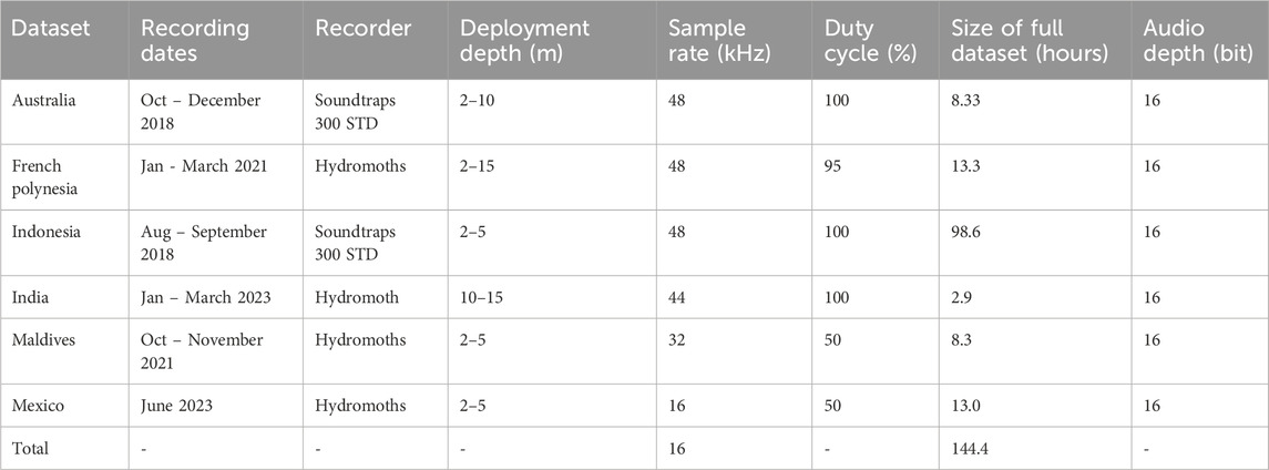
Table 1. Summary of the six underwater soundscapes datasets collected from different locations around the world between 2018 and 2023.

2.2 Fish call detection

The analytic workflow is summarized in Figure 2.

Figure 2

Figure 2. Overview of the analytical workflow for fish call detection, extraction, and analysis. Coral reef soundscape recordings were first downsampled to 16 kHz and visualized as spectrograms. A non-negative matrix factorization (NMF) algorithm was used to train models with manually selected ambient noise and snapping shrimp snaps to generate source-specific basis functions. Uniform Manifold Approximation and Projection (UMAP) was then used to cluster similar basis functions and optimize the models. In the prediction phase, semi-supervised source separation was applied to isolate fish calls. Extracted calls were analysed using two complementary approaches: (1) Geometric morphometric analysis (GMM) of the call shapes via principal component analysis (PCA), and (2) spectral and temporal feature extraction followed by UMAP to explore patterns of variation across sites.

2.2.1 Training and test datasets

For each of the six coral reef locations, we developed a separate source separation model to accommodate site-specific noise characteristics. Training datasets were curated from short snippets of soundscapes manually verified to be free of fish calls, based on both aural inspection and spectrogram review. These snippets represented approximately 2%–3% of each site’s data, except for Lakshadweep (24%), which required more extensive training due to the presence of diverse boat noise (Table 2).

Table 2

Table 2. Summary of training data and fish call detections for each dataset. The left panel shows the size of the training dataset used to build source separation models (in hours and as a percentage of the full dataset), the energy threshold values applied to spectrograms for fish call detection, and the total number of detected fish calls per dataset. These training sets were sound snippets free of any fish calls supplemented with additional selected snapping shrimp snaps. The right panel reports the subset selected and aligned for geometric morphometric analysis (GMM), and the subset used for acoustic parameter calculations.

To address false detection of snapping shrimp snaps as fish calls in preliminary analyses, we compiled a secondary training dataset comprising 80–150 manually extracted shrimp snaps per site. These were combined with the ambient noise samples to create a unified training set for each model. These inputs were used to generate distinct basis functions for background and snapping shrimp sources during the model’s learning phase. In addition to snapping shrimps, seasonal whale songs can also occur in some reef environments. During manual listening checks, we did not detect any whale songs, which are typically recorded in deeper waters and during specific seasons (e.g., Lin et al., 2021). Even if present, the long tonal units of whale song differ markedly from the short, pulsed fish calls targeted here, and would not have been retained by our detection workflow. We therefore consider whale song an unlikely source of bias in our analyses.

2.2.2 Source separation: NMF and UMAP

We used the open-source Python package soundscape_IR (Sun et al., 2022) to perform feature learning via non-negative matrix factorization (NMF). Spectrograms were generated using an FFT size of 512 samples, with a time resolution of 0.01 s, a prewhitening of 75%, and a frequency range of 100–3000 Hz, chosen to capture the majority of know fish call frequencies (Looby et al., 2022).

For each recording in the training dataset, the model learned 15 basis functions representing characteristic spectral patterns of the background and snapping shrimp sounds. To optimise model efficiency and reduce redundancy, we applied Uniform Manifold Approximation and Projection (UMAP) (McInnes et al., 2018) which clustered similar basis functions. The resulting model retained between 40–42 representative spectral features per dataset.

2.2.3 Prediction phase and fish call detection

During the prediction phase, models applied semi-supervised learning with an adaptive learning rate (α = 0.05) and three additional basis functions allowed for real-time adaptation to novel noise conditions. The system used an energy thresholding algorithm to extract regions of interest from the spectrograms, identifying potential fish calls. After source separation using NMF, we reconstructed a spectrogram that isolated the predicted fish call components. To detect fish calls, we then applied a region-growing energy thresholding algorithm to this reconstructed spectrogram. The threshold was defined as a dataset-specific amplitude value (Table 2) applied in dB to identify contiguous regions of elevated energy. These regions of interest were further filtered by temporal characteristics: minimum duration (0.05 s), maximum duration (1.5 s), minimum interval between calls (0.01 s), and pad size (0.02 s). These parameters were selected to encompass most of the known fish calls (Looby et al., 2022). To accommodate varying signal-to-noise ratios across sites, energy thresholds were dataset-specific (Table 2).

2.2.4 Performance test

We ran a performance test to assess accuracy with a percentage of recordings which were manually annotated in Raven Pro (v 1.6.5, K. Lisa Yang Center for Conservation Bioacoustics at the Cornell Lab of Ornithology, 2024). Between 20 and 30 min of randomly selected recordings (cut in 30 s bouts) for each dataset were aurally and visually investigated in Raven Pro, with a total of 10,238 annotated fish calls. The True Positive Rate (TPR) and False Positive Rate (FPR) were calculated with the performance evaluation functions from soundscape_IR (Sun et al., 2022). While TPR measures the positives instances, FPR measures the proportion of negative instances that are incorrectly classified as “fish calls” by the model.

2.3 Geometric morphometrics and principal component analysis

We used a Geometric Morphometrics Method (GMM) to compare directly the fish calls detected in all locations. GMM is the comparative analysis of shape, which is all the geometric information contained in a configuration of points and independent of differences in position, alignment and size. The R package “SoundShape” was used to run an “eigensound” analysis, which considers the graphical representation of a sound (i.e., a spectrogram) as a complex 3D surface described by a set of points in space, which are topologically homologous to semi-landmarks in GMM (Rocha and Romano, 2021). The eigensound function allows conversion of a detected call into a dataset that can be analysed similarly to coordinate sets from geometric morphometrics methods, thus enabling the direct comparison between stereotypical calls from different species (Rocha and Romano, 2021).

We followed the methods as per Rocha and Romano (2021). The detected fish calls were first aligned at the beginning of a sound window with the “align.wave” function of the ‘SoundShape’ package, with a sound window of 1.5 s, and time gaps at the beginning and end of 0.5%. A relative amplitude of −10 dB was used as a criterion for placement. Sounds were excluded from the GMM analysis if the alignment step failed to detect any significant energy contours within the defined frequency range and dB threshold (e.g., due to poor signal-to-noise ratio or ambiguous structure). These failures resulted in incomplete or empty aligned clips (final number of calls used in the GMM shown in Table 2). Across all datasets, these alignment failures accounted for approximately 51% of total detections. We verified that these excluded calls did not differ significantly from the retained sample in terms of duration or dominant frequency (Supplementary Material), supporting that the GMM analysis was not strongly biased toward a particular subset of calls.

Before running the “eigensound” function, the sampling grid was defined for semi-landmark acquisition: 97 × 23 cells per side were chosen bearing a dimensionality reduction from the dimensions of the spectrograms. Comparable semi-landmarks coordinates were then acquired using the 3D-analysis “eigensound” function, with a logarithmic scale on the time (x-axis) to emphasise the short-duration calls whilst also encompassing the long ones (Rocha and Romano, 2021). Finally, a Principal Component Analysis (PCA) was performed for dimensionality reduction on shape data. PCA was applied to the aligned spectrogram semilandmark coordinates using the prcomp function on the 2D matrix output of the geomorph package (Adams and Otárola-Castillo, 2013) after shape extraction with the eigensound function. Data were centered but not scaled prior to PCA, using default settings. Five principal components were kept that each explained more than 5% and together more than 50% of the variance.

2.4 Acoustic parameters and UMAP

We calculated various acoustic features for each detected fish call: lowest, highest and dominant frequency, duration and kurtosis. The lowest and highest frequency of each call was retrieved from the “sounscape_IR” detection log files, based on the bounding box of the signal in the spectrogram. Dominant frequency was estimated using the fpeaks function from the R package “seewave” (Sueur et al., 2012), which identifies spectral peaks in the frequency domain. Duration was computed using the duration function, which calculates the time difference between the start and end points of the signal envelope. Kurtosis was computed with kurtosis function of the R package “e1071” (Meyer et al., 2023). To reduce the risk of inaccurate extraction of these parameters in complex recordings, we applied strict inclusion criteria. We removed any calls where the dominant frequency or duration could not be reliably estimated (i.e., no peak frequencies or envelope detected and algorithms failed). In total, only 45 calls were excluded on this basis, representing a negligible fraction of the total calls detected, and thus unlikely to have biased our dataset. We also visually and aurally validated a representative subset (∼100 detected calls) of the data to confirm the accuracy of this parameter extraction.

For the next analysis (UMAP), the number of Indonesian calls was reduced from 71,854 to 23,015 by random subsampling, to mitigate the risk of overrepresentation and ensure a more balanced contribution from each region. The Indonesian dataset contained an order of magnitude more calls than others, which could otherwise dominate the variance structure of the UMAP. The number of calls parametrised for each dataset is shown in Table 2.

A UMAP was then computed with the following variables for each of the 80,994 calls: dominant frequency, duration, kurtosis, highest frequency and lowest frequency. These features were then standardised using z-score transformation (mean = 0, SD = 1). The goal of this dimension reduction was to explore whether variation in fish call acoustic characteristics (e.g., frequency, duration, kurtosis) was structured by environmental and temporal factors, including dataset origin, time of day, and lunar cycle. UMAP was selected for its ability to preserve local and global structure in high-dimensional data and applied to the scaled dataset (number of neighbours = 20, minimum distance = 0.1). The resulting two-dimensional embedding was used to visualise acoustic variation among recordings. In addition to standard scatterplots of the UMAP embedding, we generated 1D histograms and density plots of UMAP1 and UMAP2 dimensions to compare the distributions of embedded points across sites (referred to here as “datasets”). This approach highlights similarities or differences in acoustic structure between locations, even when scatterplots show visual overlap.

We also plotted the UMAP embedding in relation to the moon phase and the time of the day of each call. Moon phase was calculated with the python library “skyfield” (Rhodes, 2019) which issued the phase of the moon in degree (0° is new moon and 180° is full moon) for the date and time of each call. The time of the day (local time) was categorised into dawn (04:00–07:00), midday (07:00–16:00), dusk (16:00–19:00), and night (19:00–04:00).

In summary, we conducted two distinct analyses to explore variation in fish calls at different levels. The PCA was based solely on geometric morphometric data extracted from spectrogram shapes, allowing us to investigate variation in call form independently of recording context. The UMAP combined acoustic parameters with environmental and temporal metadata to explore broader multivariate patterns in call structure and occurrence. Together, these two approaches provided a complimentary perspective on the drivers of call diversity across the sampled reef soundscapes.

3 Results

3.1 Fish call detections

From the 144 h of recordings, a total of 120,634 fish calls were detected (Table 2), showcasing the wide diversity in vocalisations (examples in Figure 3). The performance test showed a FPR lower than 4% for all models (Table 3). The TPR was poor (<35%) for all datasets, likely due to the complexity of coral reef soundscapes, highlighting that the current source separation models only captured a portion of fish calls. In our semi-supervised framework, we prioritised a low FPR over a high TPR. The high energy thresholds employed minimised false positives but inevitably reduced the TPR. This trade-off ensured that the subset of calls retained for downstream analyses consisted of high-SNR fish sounds, providing a reliable basis for comparative analyses across datasets.

Figure 3

Figure 3. Example spectrograms and waveforms from fish calls automatically detected at each location (Australia, French Polynesia, India, Indonesia, Maldives, Mexico). Spectrograms computed with a 512 sample window and 70% overlap, sampling rate 16 kHz. Generated with R package seewave (Sueur et al., 2012).

Table 3

Table 3. Performance evaluation of fish call detection models across six datasets. Manual annotations were used to assess the accuracy of model predictions, with total annotated duration, number of manually detected calls, and number of model-detected calls reported per site. The energy threshold used for each site’s detection is indicated. Detection accuracy is summarised using the False Positive Rate (FPR) and True Positive Rate (TPR).

To assess whether the detection model introduced bias by selectively identifying certain types of calls, we compared the acoustic characteristics of true positives (TP) and false negatives (FN) in the test set. This analysis, detailed in Supplementary Material, showed that while FN calls had significantly lower signal-to-noise ratios, their durations and spectral features (low and high frequency bounds) did not differ significantly from TP calls. This suggests that the model predominantly missed quieter calls but did not systematically exclude specific call types, supporting the representativeness of the detected calls for downstream diversity analyses. In summary, the source separation models achieved low FPR, capturing only a subset of all fish calls present. The detected calls are predominantly those with high energy, tonal structure, and limited spectral overlap with background noise (e.g., snapping shrimp, boat engines). As such, the dataset likely underrepresents low-amplitude, broadband, or irregular call types. Our findings therefore reflect patterns within this detectable subset of calls, and we interpreted the results with this detection bias in mind.

3.2 Geometric morphometrics method

The summary of the GMM PCA is shown in Table 4. Of the 25,622 components, five were selected to run the analysis (Table 4), and the two major components used for data visualisation. The resulting ordination plot represents 33% of the whole variance in the dataset. Figure 4 shows the ordination analysis acquired for the different datasets.

Table 4

Table 4. Summary of the first five principal components from the PCA, conducted on 25,622 fish calls using geometric morphometric data derived from spectrogram outlines. The table reports the standard deviation of each component, the proportion of variance explained, and the cumulative variance across components. PCA was performed on extracted 2D semilandmark coordinates, with no contextual or environmental variables included in this analysis.

Figure 4

Figure 4. Principal Component Analysis (PCA) ordination plot of fish calls (n = 25,622) based on the 3D shape of their spectrogram. Points are color-coded by dataset (location). Due to high point density and overlap, dataset centroids are displayed with larger labelled points to summarize the central tendency of each location in PCA space. The plot shows the first two principal components (Dim1 and Dim2), which explain 33% of the total variance in the dataset. Ellipses represent 95% confidence intervals.

Visualisations of the hypothetical consensus sound shape were designed to represent the variation embedded in each PC axis which are equivalent to warp grids in shade space from GMM studies (Figure 5). The mean plot shape represents the ‘consensus’; i.e., the mean deformations. The mean fish call detected (Figure 5a) was made of two short bursts at low frequencies (around 500–900 Hz) separated by about 0.5 s, with possible harmonics showing at higher frequencies (∼1500 Hz). The minimum deformations along PC1 (Figure 5b) illustrate the sound surface at one end of the PC1 axis, i.e., one extreme of shape variation. In contrast, the maximum deformations along PC1 show the shape at the opposite end of the same axis, i.e., representing the opposite extreme.

Figure 5

Figure 5. Hypothetical sound surfaces generated from geometric morphometric analysis of fish calls: (a) Mean shape (consensus) configuration across all calls; (b) minimum deformations (representing one extreme of shape variation); and (c) maximum deformations (representing the opposite extreme) along principal component 1. The surfaces were produced using the hypo.surf function from the R SoundShape package.

3.3 Acoustic parameters

Using the calculated acoustic parameters for each dataset (Table 5), UMAP was used to explore patterns across the different locations. The UMAP projection revealed that acoustic features of fish sounds formed a continuous, largely overlapping cloud in the reduced two-dimensional space (Figure 6a). No distinct clusters corresponding to specific datasets were observed in the UMAP scatterplot, suggesting broadly similar acoustic structures across sites. The UMAP projection revealed a main cluster encompassing the majority of calls, along with smaller, more discrete “islands” of points. These peripheral clusters may represent distinct call types, potentially associated with specific taxa or behavioural contexts. While our unlabelled dataset does not allow taxonomic assignment, the presence of these groupings suggests acoustic differentiation that warrants targeted annotation in future studies.

Table 5

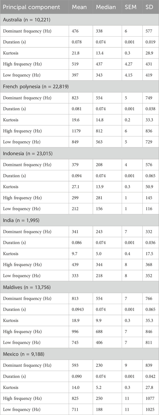
Table 5. Acoustic parameters for the calls for each dataset. SEM: standard error of the mean; SD: standard deviation.

Figure 6

Figure 6. (a) Uniform Manifold Approximation and Projection (UMAP) projection of fish calls (n= 80,994) based on five different acoustic metrics, colour-labelled by location. Density plots for UMAP1 (b) and UMAP2 (c) for each dataset (i.e., sites). UMAP projections colour-labelled by (d) moon phase (in degrees, where 0° is new moon and 180° is full moon) and by (e) time of day (dawn, dusk, midday or night).

To further explore potential site-level differences, we compared the distribution of embedded points along each UMAP dimension. Histograms and density plots for UMAP1 and UMAP2 revealed broadly overlapping distributions among datasets, with overlapping peak locations and spreads. These patterns further support the quantitative analyses (PCA and geometric morphometrics), which suggested convergence in acoustic structure across regions for the detected calls. (Figures 6b,c). The moon phase (Figure 6d) or the time of the day (Figure 6e) did not reveal any specific structures in the projection either. This indicates limited separation in acoustic structure and supports the hypothesis that certain coral reef fish sounds share conserved acoustic traits across the spatial and temporal scales investigated.

4 Discussion

In this study, we analysed a total of 144 h of recordings from six different coral reef locations around the world, detecting a total of 120,634 fish calls. Using Geometric Morphometrics Methods (GMM) and Principal Component Analysis (PCA), we captured the 3D shape and spectro-temporal features of these calls. The first two components of the 3D shape analysis (GMM) explained 33% of the total variance, with calls from different geographical areas showing substantial overlap in the PCA space. This may reflect a combination of shared call features in coral reef fish soundscapes sampled in this study and limitations in morphological differentiation using the current shape descriptors. This analysis was conducted on a large set of putatively detected fish calls. Validating these patterns using a large annotated dataset, and with more biogeographical realms would be a valuable next step.

While the calls detected had a wide range of dominant frequencies (100–3000 Hz) and durations (0.05–1.5 s) – that is, the limits imposed by our detector–their three-dimensional spectro-temporal shape (time × frequency × amplitude) remained conserved and strongly overlapping across datasets. The consensus shape shown in the GMM represents the average spectro-temporal configuration across all aligned calls: it shows a unit composed of low-frequency (bandwidth: ∼ 500–700 Hz), short (0.1–0.2 s) pulses, potentially with harmonics. This could correspond to the typical knock, croak, grunt or scrape sounds produced by a variety of resident coral reef fish species (Lamont et al., 2022b), namely, low-frequency energy (typically 200–1000 Hz), short pulse durations, and in some cases, harmonic components. These similarities suggest potential functional or mechanistic convergence. For example, fishes from the families Pomacentridae (damselfishes) and Chaetodontidae (butterflyfishes), typical resident on tropical coral reefs, have been previously described as producing such calls (Tricas and Boyle, 2014; 2021; Parmentier et al., 2016; Tricas and Webb, 2016; Lobel et al., 2019). The convergence observed in dominant frequency and call duration across locations may reflect shared environmental and biological constraints. Physically, shallow reef habitats promote the use of low-frequency or broadband, short-duration pulses that propagate more effectively in cluttered, reverberant environments where high frequencies attenuate rapidly. Anatomically, many reef fish lineages rely on similar drumming muscles, swimbladder mechanisms, or pectoral-based stridulation systems that inherently produce low-frequency or broadband pulses. Ecologically, communication in noisy reef environments may select for brief, high-SNR pulse trains that maximise detectability and minimise masking. Together, these constraints could produce convergent acoustic properties even among distantly related taxa and across widely separated regions.

This high degree of overlap in the features of sounds produced by different fishes has already been described (Tricas and Boyle, 2014) and seems to characterise the sounds from sympatric populations of hundreds of species that are concentrated in small geographic areas defining coral reefs. While coral reef biodiversity can globally display clear spatial patterns, fish species among families are strongly conserved across the Indo-Pacific (Bellwood and Hughes, 2001; Maxwell et al., 2022), a trend that our call dataset confirms. Looking at biogeography at the realm scale (sensu Kulbicki et al., 2013), the calls from our study all fall within the Indo-Pacific realm, except for the Mexican dataset, which would belong to the Atlantic realm. Further work exploring the global distribution of coral reef calls should include more datasets from the Atlantic and from the Tropical Eastern Pacific realms. Therefore, although all studied regions would differ in overall species richness, their reef fish communities include broadly comparable ecological guilds and many shared dominant families (e.g., Pomacentridae, Labridae, Acanthuridae and related herbivores, various planktivorous and nocturnal families). However, differences in species composition and relative abundance among regions may contribute to variation in acoustic assemblages. Because we lacked standardised community survey data across all sites, we could not directly associate specific acoustic clusters with local fish assemblages. Incorporating ecological surveys alongside annotated acoustic datasets represents an important future direction for linking call structure to taxonomic identity.

The UMAP embedding, based on five key acoustic parameters, revealed a largely homogeneous distribution of fish calls across geographical locations, with minimal evidence of strong clustering by region. While some datasets (e.g., French Polynesia and Mexico) showed subtle shifts in their distributions, the majority of calls overlapped substantially in reduced-dimensional space. This suggests, like the previously discussed PCA, that many coral reef fish calls share similar acoustic properties regardless of origin. However, the limited but visible structure in the UMAP plots may reflect underlying variation in dominant, highest, or lowest frequencies among locations, traits that could be shaped by both species composition and environmental conditions. The subtle separations (i.e., a few “islands”) observed in the UMAP space could correspond to species- or family-specific call types that are less widely distributed than the predominant acoustic forms represented by the main cluster. These patterns may reflect ecological or phylogenetic constraints on call structure, and future work combining annotated call libraries with taxonomic information will be essential to link acoustic diversity with species identity. These small differences hint at potential mechanisms of acoustic partitioning, prompting further exploration of the spectral niches occupied by reef fishes. The importance of the frequency bandwidth of fish calls has been highlighted in previous work, as well as their separation into distinct “niches”. For example, Noble et al. (2024) used unsupervised machine learning to cluster fish sounds from a US Virgin Islands reef, and noted the stratification of the total frequency range into clusters of different frequency bands. This clustering likely promotes effective communication, probably enabling individuals to identify conspecifics better and to communicate concurrently with other species. Similar coral fish call spectral separations were observed for the coral reef soundscapes of Goa (Mahale et al., 2023) and French Polynesia (Nedelec et al., 2015). Such acoustic niche partitioning has been observed in other taxa, such as insects (Schmidt and Balakrishnan, 2015), bats (Salinas-Ramos et al., 2020) and cetaceans (Filatova, 2024). The partitioning may be spatial, where different species avoid acoustic interference by spacing themselves apart, or temporal, by vocalising at different times of the day or during different seasons.

We expected a larger contribution of time of day to some of the UMAP structure, as other studies of fish communities highlighted a strong temporal partitioning, especially between diurnal and nocturnal species (Ruppé et al., 2015; Bertucci et al., 2020). Even if some species are more active during certain periods, there could be significant overlap in calling activity across species throughout the day. However, we acknowledge that our conservative detector was most effective at capturing a predominant call type with limited temporal variability, while other call types (i.e., potentially showing stronger temporal partitioning) may have been missed. Our conclusion of weak temporal structuring should therefore be interpreted in light of this methodological constraint. Furthermore, our study did not account for different seasons, which may also influence the frequency niche partitioning, as observed in fishes from the Sciaenidae family (Luczkovich and Sprague, 2011). Some other factors may be shaping the frequency components of fish calls, like the ambient sound itself. Fish may adapt their calling frequencies based on the acoustic properties of their environment to maximise the range and clarity of their calls under specific conditions. Environmental factors such as depth, temperature or substrate type could then influence how different frequencies propagate and each condition create a competition for acoustic space. Including data from different environmental conditions could help investigate diverse acoustic niche partitioning elements.

Our fish call detection models yielded a low FPR (<4%), which met our primary aim of characterising the range of fish calls in the soundscape rather than achieving exhaustive detection. The TPR was lower (16% on average), reflecting that many calls were missed, primarily due to variable background noise and reduced detectability of lower-SNR events. Importantly, supplementary analyses showed that these missed calls did not differ systematically in spectral or temporal features, supporting that the retained dataset remains representative of the broader fish acoustic community. Nevertheless, the similarity observed among calls should be interpreted in light of these methodological constraints. Furthermore, TPR varied among locations (from 6% to 35%), suggesting that the model performed better in some soundscapes than others. While our analyses show that this variation was primarily related to SNR rather than systematic exclusion of certain call types, it may also reflect ecological differences in call composition and background noise across sites.

It is important to note that our acoustic parameters and UMAP analysis focused on broad acoustic descriptors (dominant frequency, duration, kurtosis, band edges), which capture the overall spectral–temporal envelope of calls but not the finer-scale temporal organisation of pulse trains. Many reef fish calls consist of structured sequences of pulses, where inter-pulse intervals, pulse repetition rates, and amplitude-modulation envelopes carry species-specific information and can underpin acoustic niche partitioning. Our detection approach, optimised for extracting high-SNR transients, isolates call bursts but does not resolve their internal temporal architecture. This limitation likely contributes to the convergence observed in the parameters analysed here, and future methods capable of capturing fine temporal structure may reveal additional axes of differentiation among taxa.

As calls from unidentified fish sounds are continuously recorded and sampled, our methodology presents a new way to compare between acoustic communities and explore the structure of these acoustic assemblages in the general soundscape. However, given the current detector’s limitations, we cannot claim to fully quantify heterogeneity or acoustic diversity among reefs. Future developments in detection algorithms will be essential to address this. Future work should also include comparisons with calls from different ecosystems to further examine the convergent acoustic properties we found in coral reef fish communities. For example, soundscapes from temperate reefs, mangroves, or deep coral reefs could be compared with our results. The development of underwater low-cost autonomous recording units will significantly increase the availabilities of long-term recordings of underwater soundscapes (Chapuis et al., 2021; Lamont et al., 2022a). More generally, our methodology could be applied to other animal taxa, like birds and bats, which benefit from more annotated datasets, trained detectors and classifiers (e.g., Brooker et al., 2020; Roemer et al., 2021; Dierckx et al., 2022). Similarly, with the evolution of AI and automated species identification, a phylogenetic approach could be added to our analysis. Adding phylogenetic signals to the geometric morphometric analysis of the call shape would add valuable additional power to our approach. Investigations of particular interest on the evolution of calls in coral reef fishes, and further studies on acoustic niche partitioning hypotheses will be then within reach. The importance of factors like the moon phase and time of the day may then become more prevalent, when weighted for the species correlations.

In conclusion, our study provides preliminary evidence that certain coral reef fish calls, despite geographic separation, may exhibit notable acoustic and spectro-temporal similarities. While these results are based on putatively detected signals and should be interpreted with caution, they raise important questions about the structure of coral reef soundscapes and the potential for using fish call characteristics in non-invasive monitoring of reef health (Jarriel et al., 2024). Our results also highlight the need for further methodological development. Improving detector performance to increase TPR and minimise potential biases will be essential for the wider application of this approach. Future refinements, including training on more diverse libraries of fish calls, will be critical to extend the utility of the tool for examining acoustic diversity and ecological patterns at broader scales. As technological advances make long-term passive acoustic monitoring more accessible, the integration of these methods with automatic detection (Mouy et al., 2024) and species identification holds great promise for the future of coral reef conservation. By further investigating the acoustic behaviour of fish communities across different ecosystems, we can continue to develop comprehensive soundscape-based health indicators, providing a valuable addition to traditional biodiversity assessments.

Data availability statement

The raw data supporting the conclusions of this article will be made available by the authors, without undue reservation.

Author contributions

LC: Conceptualization, Data Curation, Formal Analysis, Funding Acquisition, Investigation, Methodology, Project Administration, Resources, Software, Validation, Visualization, Writing – original draft, Writing – review and editing. T-HL: Investigation, Methodology, Software, Validation, Writing – review and editing. BW: Conceptualization, Data curation, Methodology, Resources, Writing – review and editing. TL: Conceptualization, Data curation, Resources, Writing – review and editing. RK: Data curation, Resources, Writing – review and editing. GN-M: Data curation, Resources, Writing – review and editing. AN: Data curation, Resources, Writing – review and editing. AR: Funding acquisition, Supervision, Validation, Writing – review and editing. SS: Funding acquisition, Supervision, Validation, Writing – review and editing.

Funding

The authors declare that financial support was received for the research and/or publication of this article. LC is supported by the European Union Horizon 2020 research and innovation programme under the Marie Skłodowska-Curie agreement (Grant No. 897218). THL is supported by the Grand Challenge Program Seed Grant of Academia Sinica (Grant No. AS-GCS-112-L05). TACL is supported by a Research Fellowship from the 1851 Royal Commission of the Exhibition of 1851. RK is supported by the National Geographic Society. BW is supported by a PhD studentship from the Fisheries Society of the British Isles.

Acknowledgements

We acknowledge the traditional landowners of all the locations where these recordings were made. All recordings were taken from coral reef monitoring programmes associated with other projects, which we acknowledge here. Recordings from Indonesia were originally collected as part of the monitoring program for the Mars Coral Reef Restoration Project, in collaboration with Universitas Hasanuddin. We thank Mars Sustainable Solutions for granting re-use of these recordings for this study. The original recordings were collected under an Indonesian national research permit issued by BRIN (number 108/SIP/IV/FR/2/2023), with ethical approval from BRIN and Lancaster University, and support from the Department of Marine Affairs and Fisheries of the Province of South Sulawesi, the Government Offices of the Kabupaten of Pangkep, Pulau Bontosua and Pulau Badi, and the community of Pulau Bontosua. Recordings in India were collected as part of monitoring program for fish spawning aggregations under the research permit LD-04001/2/2024-R and D-UT-LKS/46 with ethical approval from Lancaster University and support from the Department of Environment and Forests, Union Territory of Lakshadweep, India. For the Australian dataset the authors would like to acknowledge the Dingaal Aboriginal people (original land owners of Lizard Island) and thank staff from Australian Museum Lizard Island Research Station, as well as Emma Weschke and Laura Richardson. All Australian recordings were collected with ethical approval from the University of Bristol (UIN/17/074), the University of Exeter (eCLESBio000270), the Lizard Island Research Station, Great Barrier Marine Park Authority (G19/42767.1) and James Cook University (A2641), with a Queensland Department of Agriculture Fisheries and Forestry permit (200573). Mars Sustainable Solutions and Sheba Hope Grows are funding the coral reef restoration project at Fulhadhoo Island, in partnership with Fulhadhoo Island Council. The Maldives Coral Institute carried out the project under a collaboration with Save the Beach Maldives.

Conflict of interest

The authors declare that the research was conducted in the absence of any commercial or financial relationships that could be construed as a potential conflict of interest.

The author(s) declared that they were an editorial board member of Frontiers, at the time of submission. This had no impact on the peer review process and the final decision.

Generative AI statement

The authors declare that Generative AI was used in the creation of this manuscript. We used ChatGPT4 to assist with grammar and spelling in the preparation of the manuscript.

Any alternative text (alt text) provided alongside figures in this article has been generated by Frontiers with the support of artificial intelligence and reasonable efforts have been made to ensure accuracy, including review by the authors wherever possible. If you identify any issues, please contact us.

Publisher’s note

All claims expressed in this article are solely those of the authors and do not necessarily represent those of their affiliated organizations, or those of the publisher, the editors and the reviewers. Any product that may be evaluated in this article, or claim that may be made by its manufacturer, is not guaranteed or endorsed by the publisher.

Supplementary material

The Supplementary Material for this article can be found online at: https://www.frontiersin.org/articles/10.3389/frsen.2025.1522641/full#supplementary-material

References

Adams, D. C., and Otárola-Castillo, E. (2013). geomorph: an r package for the collection and analysis of geometric morphometric shape data. Methods Ecol. Evol. 4, 393–399. doi:10.1111/2041-210x.12035

CrossRef Full Text | Google Scholar

Amorim, M. (2006). “Diversity of sound production in fish,” in Communication in fishes. Editors F. Ladich, S. P. Collin, P. Moller, and B. G. Kapoor (Enfield, NH, United States: Science Publishers), 71–105.

Google Scholar

Barroso, V. R., Xavier, F. C., and Ferreira, C. E. L. (2023). Applications of machine learning to identify and characterize the sounds produced by fish. ICES J. Mar. Sci. 80, 1854–1867. doi:10.1093/icesjms/fsad126

CrossRef Full Text | Google Scholar

Bellwood, D. R., and Hughes, T. P. (2001). Regional-scale assembly rules and biodiversity of coral reefs. Science 292, 1532–1535. doi:10.1126/science.1058635

PubMed Abstract | CrossRef Full Text | Google Scholar

Bertucci, F., Maratrat, K., Berthe, C., Besson, M., Guerra, A. S., Raick, X., et al. (2020). Local sonic activity reveals potential partitioning in a coral reef fish community. Oecologia 193, 125–134. doi:10.1007/s00442-020-04647-3

PubMed Abstract | CrossRef Full Text | Google Scholar

Brooker, S. A., Stephens, P. A., Whittingham, M. J., and Willis, S. G. (2020). Automated detection and classification of birdsong: an ensemble approach. Ecol. Indic. 117, 106609. doi:10.1016/j.ecolind.2020.106609

CrossRef Full Text | Google Scholar

Chapuis, L., Williams, B., Gordon, T. A. C., and Simpson, S. D. (2021). Low-cost action cameras offer potential for widespread acoustic monitoring of marine ecosystems. Ecol. Indic. 129, 107957. doi:10.1016/j.ecolind.2021.107957

CrossRef Full Text | Google Scholar

Desiderà, E., Guidetti, P., Panzalis, P., Navone, A., Valentini-Poirrier, C., Boissery, P., et al. (2019). Acoustic fish communities: sound diversity of rocky habitats reflects fish species diversity. Mar. Ecol. Prog. Ser. 608, 183–197. doi:10.3354/meps12812

CrossRef Full Text | Google Scholar

Dierckx, L., Beauvois, M., and Nijssen, S. (2022). Advances in Intelligent Data Analysis XX, 20th International Symposium on Intelligent Data Analysis, IDA 2022, Rennes, France, April 20–22, 2022, Proceedings. Lecture Notes in Computer Science. Cham, Switzerland: Springer, 53–65.

Google Scholar

Filatova, O. A. (2024). The role of cultural traditions in ecological niche partitioning in cetaceans. Biol. Bull. Rev. 14, 133–140. doi:10.1134/s2079086424010043

CrossRef Full Text | Google Scholar

Harris, S. A., Shears, N. T., and Radford, C. A. (2016). Ecoacoustic indices as proxies for biodiversity on temperate reefs. Methods Ecol. Evol. 7, 713–724. doi:10.1111/2041-210x.12527

CrossRef Full Text | Google Scholar

Jarriel, S. D., Formel, N., Ferguson, S. R., Jensen, F. H., Apprill, A., and Mooney, T. A. (2024). Unidentified fish sounds as indicators of coral reef health and comparison to other acoustic methods. Front. Remote Sens. 5, 1338586. doi:10.3389/frsen.2024.1338586

CrossRef Full Text | Google Scholar

K. Lisa Yang Center for Conservation Bioacoustics at the Cornell Lab of Ornithology (2024). Raven Pro: Interactive Sound Analysis Software (version 1.6.5) [Computer software]. Ithaca, NY: The Cornell Lab of Ornithology. Available online at: https://www.ravensoundsoftware.com.

Google Scholar

Kulbicki, M., Parravicini, V., Bellwood, D. R., Arias-Gonzàlez, E., Chabanet, P., Floeter, S. R., et al. (2013). Global biogeography of reef fishes: a hierarchical quantitative delineation of regions. PLoS ONE 8, e81847. doi:10.1371/journal.pone.0081847

PubMed Abstract | CrossRef Full Text | Google Scholar

Lamont, T. A. C., Chapuis, L., Williams, B., Dines, S., Gridley, T., Frainer, G., et al. (2022a). HydroMoth: testing a prototype low-cost acoustic recorder for aquatic environments. Remote Sens. Ecol. Conserv. 8, 362–378. doi:10.1002/rse2.249

CrossRef Full Text | Google Scholar

Lamont, T. A. C., Williams, B., Chapuis, L., Prasetya, M. E., Seraphim, M. J., Harding, H. R., et al. (2022b). The sound of recovery: coral reef restoration success is detectable in the soundscape. J. Appl. Ecol. 59, 742–756. doi:10.1111/1365-2664.14089

CrossRef Full Text | Google Scholar

Lin, T., and Kawagucci, S. (2024). Acoustic twilight: a year-long seafloor monitoring unveils phenological patterns in the abyssal soundscape. Limnol. Oceanogr. Lett. 9, 23–32. doi:10.1002/lol2.10358

CrossRef Full Text | Google Scholar

Lin, T.-H., Tsao, Y., Wang, Y.-H., Yen, H.-W., and Lu, S.-S. (2017). Computing biodiversity change Via a soundscape monitoring network. 2017 Pac Neighborhood Consort. Annu. Conf. Jt. Meet. Pnc, 128–133. doi:10.23919/pnc.2017.8203533

CrossRef Full Text | Google Scholar

Lin, T.-H., Tsao, Y., and Akamatsu, T. (2018). Comparison of passive acoustic soniferous fish monitoring with supervised and unsupervised approaches. J. Acoust. Soc. Am. 143, EL278–EL284. doi:10.1121/1.5034169

PubMed Abstract | CrossRef Full Text | Google Scholar

Lin, T.-H., Akamatsu, T., Sinniger, F., and Harii, S. (2021). Exploring coral reef biodiversity via underwater soundscapes. Biol. Conserv. 253, 108901. doi:10.1016/j.biocon.2020.108901

CrossRef Full Text | Google Scholar

Lobel, P. S., Kaatz, I. M., and Rice, A. N. (2019). Reproduction and sexuality in marine fishes. Patterns Process., 307–386. doi:10.1525/9780520947979-013

CrossRef Full Text | Google Scholar

Looby, A., Cox, K., Bravo, S., Rountree, R., Juanes, F., Reynolds, L. K., et al. (2022). A quantitative inventory of global soniferous fish diversity. Rev. Fish. Biol. Fish. 32, 581–595. doi:10.1007/s11160-022-09702-1

CrossRef Full Text | Google Scholar

Luczkovich, J., and Sprague, M. (2011). Speciation and sounds of fishes: dividing up the bandwidth. Proc. Meet. Acoust. 12, 010003. doi:10.1121/1.4718869

CrossRef Full Text | Google Scholar

Mahale, V. P., Chanda, K., Chakraborty, B., Salkar, T., and Sreekanth, G. B. (2023). Biodiversity assessment using passive acoustic recordings from off-reef location—Unsupervised learning to classify fish vocalization. J. Acoust. Soc. Am. 153, 1534–1553. doi:10.1121/10.0017248

PubMed Abstract | CrossRef Full Text | Google Scholar

Malfante, M., Mars, J. I., Mura, M. D., and Gervaise, C. (2018). Automatic fish sounds classification. J. Acoust. Soc. Am. 143, 2834–2846. doi:10.1121/1.5036628

PubMed Abstract | CrossRef Full Text | Google Scholar

Maxwell, M. F., Leprieur, F., Quimbayo, J. P., Floeter, S. R., and Bender, M. G. (2022). Global patterns and drivers of beta diversity facets of reef fish faunas. J. Biogeogr. 49, 954–967. doi:10.1111/jbi.14349

CrossRef Full Text | Google Scholar

McInnes, L., Healy, J., and Melville, J. (2018). UMAP: uniform manifold approximation and projection for dimension reduction. arXiv. doi:10.48550/arxiv.1802.03426

CrossRef Full Text | Google Scholar

Meyer, D., Dimitriadou, E., Hornik, K., Weingessel, A., and Leisch, F. (2023). e1071: Misc functions of the department of statistics. TU Wien Probab. Theory Group (Formerly E1071). doi:10.32614/CRAN.package.e1071

CrossRef Full Text | Google Scholar

Minello, M., Calado, L., and Xavier, F. C. (2021). Ecoacoustic indices in marine ecosystems: a review on recent developments, challenges, and future directions. ICES J. Mar. Sci. 78, fsab193. doi:10.1093/icesjms/fsab193

CrossRef Full Text | Google Scholar

Mooney, T. A., Iorio, L. D., Lammers, M., Lin, T.-H., Nedelec, S. L., Parsons, M., et al. (2020). Listening forward: approaching marine biodiversity assessments using acoustic methods. Roy. Soc. Open Sci. 7, 201287. doi:10.1098/rsos.201287

CrossRef Full Text | Google Scholar

Mouy, X., Archer, S. K., Dosso, S., Dudas, S., English, P., Foord, C., et al. (2024). Automatic detection of unidentified fish sounds: a comparison of traditional machine learning with deep learning. Front. Remote Sens. 5, 1439995. doi:10.3389/frsen.2024.1439995

CrossRef Full Text | Google Scholar

Nedelec, S., Simpson, S., Holderied, M., Radford, A., Lecellier, G., Radford, C., et al. (2015). Soundscapes and living communities in coral reefs: temporal and spatial variation. Mar. Ecol. Prog. Ser. 524, 125–135. doi:10.3354/meps11175

CrossRef Full Text | Google Scholar

Noble, A. E., Jensen, F. H., Jarriel, S. D., Aoki, N., Ferguson, S. R., Hyer, M. D., et al. (2024). Unsupervised clustering reveals acoustic diversity and niche differentiation in pulsed calls from a coral reef ecosystem. Front. Remote Sens. 5, 1429227. doi:10.3389/frsen.2024.1429227

CrossRef Full Text | Google Scholar

Parmentier, E., Lecchini, D., and Mann, D. A. (2016). “Sound production in damselfishes,” in Biology of damselfishes. Editors B. Frederich, and E. Parmentier (Florida: Boca Raton: CRC Press, Taylor & Francis), 204–228.

Google Scholar

Parsons, M. J. G., Lin, T.-H., Mooney, T. A., Erbe, C., Juanes, F., Lammers, M., et al. (2022). Sounding the call for a global library of underwater biological sounds. Front. Ecol. Evol. 10, 810156. doi:10.3389/fevo.2022.810156

CrossRef Full Text | Google Scholar

Radford, C., Stanley, J., Tindle, C., Montgomery, J., and Jeffs, A. (2010). Localised coastal habitats have distinct underwater sound signatures. Mar. Ecol. Prog. Ser. 401, 21–29. doi:10.3354/meps08451

CrossRef Full Text | Google Scholar

Radford, C. A., Stanley, J. A., and Jeffs, A. G. (2014). Adjacent coral reef habitats produce different underwater sound signatures. Mar. Ecol. Prog. Ser. 505, 19–28. doi:10.3354/meps10782

CrossRef Full Text | Google Scholar

Raick, X., Iorio, L. D., Lecchini, D., Bolgan, M., and Parmentier, E. (2023). “to Be, or not to be”: critical assessment of the use of α-Acoustic diversity indices to evaluate the richness and abundance of coastal marine fish sounds. J. Ecoacoustics 7, 1. doi:10.35995/jea7010001

CrossRef Full Text | Google Scholar

Rhodes, B. (2019). Skyfield: high precision research-grade positions for planets and Earth satellites generator. Astrophys. Source Code Libr. Available online at: https://github.com/skyfielders/python-skyfield.

Google Scholar

Rocha, P. C., and Romano, P. S. R. (2021). The shape of sound: a new R package that crosses the bridge between bioacoustics and geometric morphometrics. Methods Ecol. Evol. 12, 1115–1121. doi:10.1111/2041-210x.13580

CrossRef Full Text | Google Scholar

Roemer, C., Julien, J., Ahoudji, P. P., Chassot, J., Genta, M., Colombo, R., et al. (2021). An automatic classifier of bat sonotypes around the world. Methods Ecol. Evol. 12, 2432–2444. doi:10.1111/2041-210x.13721

CrossRef Full Text | Google Scholar

Ross, S. R. P.-J., O’Connell, D. P., Deichmann, J. L., Desjonquères, C., Gasc, A., Phillips, J. N., et al. (2023). Passive acoustic monitoring provides a fresh perspective on fundamental ecological questions. Funct. Ecol. 37, 959–975. doi:10.1111/1365-2435.14275

CrossRef Full Text | Google Scholar

Ruppé, L., Clément, G., Herrel, A., Ballesta, L., Décamps, T., Kéver, L., et al. (2015). Environmental constraints drive the partitioning of the soundscape in fishes. Proc. Natl. Acad. Sci. 112, 6092–6097. doi:10.1073/pnas.1424667112

PubMed Abstract | CrossRef Full Text | Google Scholar

Salinas-Ramos, V. B., Ancillotto, L., Bosso, L., Sánchez-Cordero, V., and Russo, D. (2020). Interspecific competition in Bats: state of knowledge and research challenges. Mammal. Rev. 50, 68–81. doi:10.1111/mam.12180

CrossRef Full Text | Google Scholar

Sattar, F., Cullis-Suzuki, S., and Jin, F. (2016). Identification of fish vocalizations from ocean acoustic data. Appl. Acoust. 110, 248–255. doi:10.1016/j.apacoust.2016.03.025

CrossRef Full Text | Google Scholar

Schmidt, A. K. D., and Balakrishnan, R. (2015). Ecology of acoustic signalling and the problem of masking interference in insects. J. Comp. Physiol. A 201, 133–142. doi:10.1007/s00359-014-0955-6

PubMed Abstract | CrossRef Full Text | Google Scholar

Stratoudakis, Y., Vieira, M., Marques, J. P., Amorim, M. C. P., Fonseca, P. J., and Quintella, B. R. (2024). Long-term passive acoustic monitoring to support adaptive management in a sciaenid fishery (tagus Estuary, Portugal). Rev. Fish. Biol. Fish. 34, 491–510. doi:10.1007/s11160-023-09825-z

CrossRef Full Text | Google Scholar

Sueur, J., Aubin, T., and Simonis, C. (2012). Seewave, a free modular tool for sound analysis and synthesis. Bioacoustics 18, 213–226. doi:10.1080/09524622.2008.9753600

CrossRef Full Text | Google Scholar

Sun, Y., Yen, S., and Lin, T. (2022). soundscape_IR: a source separation toolbox for exploring acoustic diversity in soundscapes. Methods Ecol. Evol. 13, 2347–2355. doi:10.1111/2041-210x.13960

CrossRef Full Text | Google Scholar

Tricas, T., and Boyle, K. (2014). Acoustic behaviors in Hawaiian coral reef fish communities. Mar. Ecol. Prog. Ser. 511, 1–16. doi:10.3354/meps10930

CrossRef Full Text | Google Scholar

Tricas, T., and Boyle, K. (2021). Parrotfish soundscapes: implications for coral reef management. Mar. Ecol. Prog. Ser. 666, 149–169. doi:10.3354/meps13679

CrossRef Full Text | Google Scholar

Tricas, T. C., and Webb, J. F. (2016). Acoustic communication in butterflyfishes: anatomical novelties, physiology, evolution, and behavioral ecology. Adv. Exp. Med. Biol. 877, 57–92. doi:10.1007/978-3-319-21059-9_5

PubMed Abstract | CrossRef Full Text | Google Scholar

Vieira, M., Fonseca, P. J., Amorim, M. C. P., and Teixeira, C. J. C. (2015). Call recognition and individual identification of fish vocalizations based on automatic speech recognition: an example with the Lusitanian toadfish. J. Acoust. Soc. Am. 138, 3941–3950. doi:10.1121/1.4936858

PubMed Abstract | CrossRef Full Text | Google Scholar

Vieira, M., Pereira, B. P., Pousão-Ferreira, P., Fonseca, P. J., and Amorim, M. C. P. (2019). Seasonal variation of captive meagre acoustic signalling: a manual and automatic recognition approach. Fishes 4, 28. doi:10.3390/fishes4020028

CrossRef Full Text | Google Scholar