Long-term evolution of forest cover in the Pacific coast of Ecuador (1960–2019): a comparison of Land Use/Land Cover (LULC) remote sensing products

Ecosystem services provided by forests are increasingly threatened by anthropogenic and climatic disturbances. International initiatives to reduce greenhouse gas emissions from forest disturbances, such as Reducing Emissions from Deforestation and Degradation+ (REDD+), require robust quantifications of the dynamics and extent of Land Use/Land Cover (LULC). However, no study present yet a comparative synthesis of existing LULC products and long-term landscape evolution on the Pacific Slope and Coast of Ecuador (EPSC). In addition, previous studies on the evolution of the forest cover in the EPSC were achieved on small regions and short time-scales, never analysing before the 1990s. In this context, we conducted a long-term study of landscape dynamics at the scale of the EPSC on the last 6 decades (1960-2019). In addition, we propose a comparative synthesis of the main land use databases from remote sensing. To do this, we compared six LULC databases (HILDA+, ESA-CCI, MODIS, GLCLUC, TMF, GFC) derived from remote sensing using the Ecuadorian Ministry of Environment and Water (MAATE) LULC dataset as a reference. This comparison was performed with confusion matrices. Three metrics are calculated from the confusion matrices: Accuracy, F1-score and MCC. HILDA+ and TMF products showed the best agreement with the MAATE map (F1-score of 0.63 and 0.65, respectively). HILDA + captured net forest cover losses better than TMF (65% vs 27% of the net losses recorded by MAATE). Of the six databases analysed, HILDA+ was identified as the product with the best correlation with the Ministry’s LULC maps. Therefore, HILDA+ was chosen to analyse deforestation since 1960 in the EPSC. The major limitation encountered using HILDA+ is the coarse spatial resolution of 1 km. Yet, four deforestation phases were identified in the EPSC over 1960–2019. They reflect the historical, social, political, and climatical context of each ecosystem. Over the entire period (1960-2019), forest cover decreased by 43.9%. Since the 1960s, tropical rainforest areas declined by a third. Dry and transitional tropical forests lost more than half their area.

1 Introduction

Forests provide numerous ecosystem services such as climate and water regulation, erosion prevention and carbon storage (Daily, 1998; Krieger, 2001; García-Nieto et al., 2013). However, forest ecosystems are threatened by anthropogenic pressures, leading to land use changes and promoting deforestation (Barlow et al., 2016), with multiple consequences such as species extinction (Whitmore and Sayer, 1992; Giam, 2017), emissions of carbon and other greenhouse gases (Eva et al., 2012), soil erosion and consequent loss of organic matter (Ochoa-Cueva et al., 2015). Forests are also affected by climate change and subject to extreme weather events (França et al., 2020) that generate climatic stress for trees (Anderegg et al., 2012; Scholze et al., 2006) and that disrupt the ecological functions of forest ecosystems. On a global scale, between 1990 and 2020, forest cover decreased from 32.5% to 30.8% of total land area (UN Environment Programme and Food and Agriculture Organization of the United Nations, 2020). The greatest losses occurred in South America and Africa. In South America, Ecuador has the highest rate of deforestation (Mosandl et al., 2008; Armenteras et al., 2017), and the forests located on the Pacific Slope and Coast of Ecuador (EPSC) are the most threatened by deforestation and are considered a biodiversity hotspot (Myers, 1988). On the EPSC, the anthropogenic pressures responsible for deforestation are mainly linked to the conversion of forest to cropland. According to the Land Use/Land Cover (LULC) map of the Ministry of Environment and Water of Ecuador (MAATE) in 2022, 73.9% of cropland was on the EPSC. Climatic disturbances are mainly linked to the ENSO phenomena, which cause extreme flooding and drought in the EPSC (Vicente-Serrano et al., 2017).

In this context, international initiatives such as the Reducing Emissions from Deforestation and Forest Degradation (REDD+) project (Matthews et al., 2014), whose main objective is to reduce greenhouse gas emissions linked to deforestation (Goetz et al., 2015), have showed the importance of better quantifying the process of forest dynamics in tropical zones. REDD+ was implemented nationally in Ecuador through the “Bosques para Buen vivir” plan (MAATE, 2017). Through this project, MAATE expressed the importance of having a long-term monitoring of deforestation process and provided eight national LULC maps between 1990 and 2022.

Studies comparing land use and land cover databases in South America mainly focus on emblematic regions such as Brazil (Souza et al., 2020), the Amazon basin (Ometto et al., 2016; Neves, A. K. et al., 2020) or even the Gran Chaco (Graesser et al., 2022; Baumann et al., 2017; Fehlenberg et al., 2017). These studies were generally based on the use of the main LULC products available at continental or global scales, such as MapBiomas, Global Forest Change, MODIS Land Cover, ESA CCI Land Cover or PRODES. The study of deforestation in South America therefore focuses on these key regions. In the Brazilian Amazonian, Wagner et al. (2022) used high-resolution images (5 m, Planet NICFI) and a U-Net network to map tree cover loss in the state of Mato Grosso between 2015 and 2021, revealing an increase in deforestation and significant discrepancies with the Global Forest Change data. Blaschke et al. (2023) shows a weakening of the resilience of the Amazon rainforest based on spatial trends in optical/radar satellite data. In the Peruvian Amazon, Móstiga et al. (2024) estimate a loss of 3.4 M ha between 2000 and 2020. In the Andes and their foothills, although less documented than in the Amazon, studies particularly in dry eco-regions and high altitude areas. For example, Rodríguez-Echeverry (2023) report a 45% loss of inter-Andean dry forest in the Río Chota watershed between 1991 and 2017, an annual deforestation rate of 2.3%, mainly due to agricultural expansion. Finally, Juarez et al. (2024) identify rainfall (41%) and temperature (20%) as the main factors of deforestation in the Peruvian Andes between 2000 and 2020, while highlighting the permanent role of agriculture as an underlying engine. An intensification in LULC changes, and especially deforestation, was observed in Piura Basin, Peruvian Pacific slope, due to the intensification of climate extremes between 2012 and 2022, compared to 2001–2011 (Castillón, et al., 2025). The study by Romero-Muñoz et al. (2020) shows that deforestation, combined with hunting, affects 40% of the area of the South American Chaco, with strong synergistic consequences on biodiversity (increased habitat loss, increased human pressures) Ecuador remains relatively little studied, particularly on the entire Pacific slope, where work comparing data sets is rare. One of the only studies covering this territory is that of Ferrer Velasco et al. (2022), which highlights major discrepancies between databases in regions of piedmont and humid tropical coastal forests.

The studies by Sierra et al. (2021) and González-Jaramillo et al. (2016) at national level agree in identifying the coastal biome as the most affected by deforestation compared to the Andean regions and the Amazon basin. The study by Sierra et al. (2021) used national LULC maps of MAATE and showed that, in 2018, coastal forests had retained only 27% of their original area in 1990. The analysis showed that the five most threatened and least well-preserved forest ecosystems are located on the coast. The analysis by González-Jaramillo et al. (2016) of NOAA-AVHRR images acquired on three dates: 1986, 2001 and 2008, has identified the coastal biome as the area most affected by deforestation, with forest cover falling from 15.2% to 1.9%. Other studies focused on specific areas of the EPSC. Rivas et al. (2021), focused on the seasonal dry forests of the coastal biome and showed that only 27.04% of their original area remained in 1990. This latter study showed that semi-deciduous forests present the highest levels of fragmentation and require more effective protection. These fragmentation processes and their consequences for biodiversity were studied by Rivas et al. (2024) which explains why global forest connectivity fell from 25% to 13.69% between 1990 and 2018. Kleemann et al. (2022) highlighted the spatial patterns of deforestation in and around protected areas on the scale of continental Ecuador and showed that 25.5% of total deforestation between 1990 and 2018 took place around protected areas (up to 10 km around) and that the areas in the immediate vicinity (5 km) of areas with a high level of protection were the most affected. Other studies focused on small areas in specific regions of the south or north of Ecuador. Tapia-Armijos et al. (2015) analysed deforestation in the provinces of Loja and Zamora Chinchipe over 3 years 1976, 1989 and 2008. The study found a 46% loss in the original forest cover in southern Ecuador in 2008. Sierra and Stallings (1998) analysed the dynamics of deforestation in northwestern Ecuador between 1983 and 1995 and found that the forests in this region could disappear completely within 30–35 years.

Thus, previous studies show that few have analysed deforestation at the scale of the EPSC and that they have generally focused on small specific areas. Previous studies based on MAATE LULC maps do not analyse deforestation before the 1990s. In addition, most remote sensing studies that monitor forests in EPSCs are based on satellite images taken in a few specific years and that do not allow us to go back before the 1980s. The previous studies do not present a continuous monitoring of the deforestation process. These studies do not present a continuous analysis over time and over the long term of the deforestation process at the scale of the EPSC. None of the previous studies provides a comparative synthesis of existing land use products.

In this study, we propose the first comparative synthesis of six existing land use products at the EPSC scale. Unlike previous studies, we can analyse the deforestation process with an annual temporal resolution from the 1960s, whereas most studies only go back to the 1990s.

Here, we reconstructed the landscape dynamics over 6 decades (1960-2019) by analysing forest cover evolution with an annual time resolution at EPSC scale. We have established the different spatio-temporal dynamics of the deforestation process at the scale of bioclimatic zones. We have recontextualized the deforestation process in the political, social, economic and climate context to better understand the impacts of disruptive events (anthropogenic and climatic) on forest ecosystems. We used HIstoric Land Dynamics Assessment+ (HILDA+), a long-term remote sensing product validated with MAATE reference LULC data.

2 Study area

Ecuador (81.03°W–75.16°W, 1.48°N–5.04°S) is located in the north-west of South America, between Colombia and Peru. The country is composed of three main regions: the Pacific coast to the west (Costa) and the Amazon plain to the east (Oriente), separated by the Andes Mountains (Sierra). The Sierra region is bordered by two main chains separated by the inter-Andean zone characterized by several valleys in which the capital of Ecuador, Quito is located. The topographical and climatic characteristics of these different regions influence the spatial distribution and type of forest cover. In 2022, the Amazon basin, home to tropical rain forests, accounted for 76,4% of the country’s forest cover according to the MAATE (http://ide.ambiente.gob.ec/mapainteractivo). The rest of the forest cover is mostly located in the Pacific slope and coast of Ecuador (EPSC) considered a biodiversity hotspot (Myers, 1988).

Our study area is the EPSC which extends from the Pacific Ocean to the Andean foothills on an area of ∼116,436 km², covering 47% of the Ecuadorian territory. In 2022, according to the MAATE, 59,6% of the EPSC is occupied by agricultural land, and forest cover represents 24,7% (Figure 1a). In the EPSC, large bioclimatic differences are responsible for a wide diversity of landscapes and ecosystems (Figure 1b). The coastal region is delimited on the western part by the low altitude Coastal Cordillera (1° N to 2° S, with a maximum altitude of 860 m. a.s.l) and is exposed to dry climatic conditions with annual rainfall below 600 mm/year (Erazo et al., 2018). It is predominantly covered with tropical dry forests, but also deciduous and semi deciduous forests (Diertl, 2010). Around the Andean foothills, rainfall can reach 2,000 mm/year and the rain-fed bioclimate is home to tropical rainforests, with evergreen forests stretching to the north of the country. Beyond the foothills of the Andes, at the highest altitudes, forest cover gives way to páramo vegetation, an ecosystem of tropical alpine grasslands characterized by shrub communities. In the north of the country, at altitudes above 4,000 m. a.s.l, there is grass-páramo vegetation. To the south, the tree line is at an altitude of over 2,500 m. a.s.l, above which lies shrub-páramo vegetation. This difference is due to the Andean depression located between southern Ecuador and northern Peru (Richter, 2003).

Figure 1

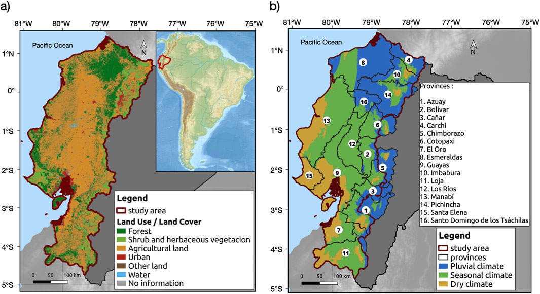
Figure 1. (a) LULC for the year 2022 (MAATE) in the EPSC, delineated in red, in the west of Ecuador. (b) Forest characteristics differ according to three bioclimatic zones ranging from dry tropical to humid tropical climate. EPSC encompassed 16 provinces of the 24 of the country.

3 Materials and methods

3.1 Datasets

3.1.1 Earth observation-based products

Four LULC and two forest cover change products were selected for this study as they offer global spatial coverage, a medium (1 km-300 m) to high (30 m) spatial resolutions and a long-term temporal coverage (longer than 20 years). Most of them are available at a temporal resolution of 1 year. All databases are freely available. The characteristics of the products are summarized in Table 1.

Table 1

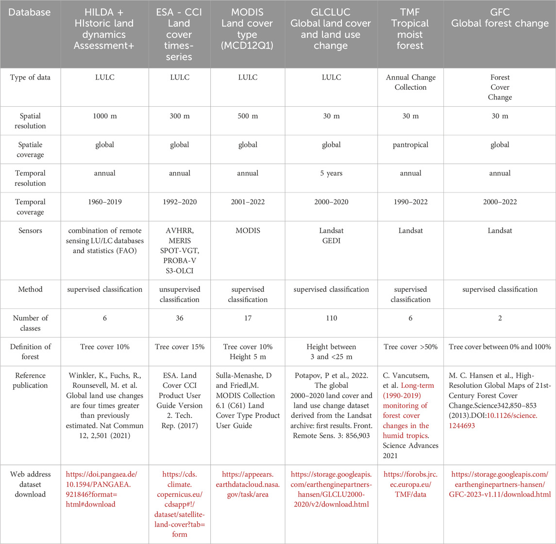
Table 1. Characteristics of land use and forest cover change databases derived from remote sensing products and used in this study.

Two types of data are available: Land Use/Land Cover (LULC) maps HIstoric Land Dynamics Assessment+ (HILDA+), ESA Climatic Change Initiative Land Cover (ESA-CCI LC), Moderate Resolution Imaging Spectroradiometer (MODIS) Land Cover Type, Global Land Cover and Land Use Change (GLCLUC) and forest cover change maps Tropical Moist Forest (TMF), Global Forest Change (GFC). All of them include Earth Observation (EO) data, mostly originating from multispectral images but also from LiDAR-derived canopy heights derived from GEDI in the case of GLCLUC (Potapov et al., 2022). HILDA + results from the combination of multi-source land cover databases and FAO statistics (Winkler et al., 2021). The products are based on supervised classification approaches, except ESA-CCI LC which is based on an unsupervised classification. For the four LULC databases, the number of land use classes ranges from 6 to 110. ESA CCI and MODIS distinguish between different types of forest cover (Evergreen Needleleaf/Broadleaf Forests, Deciduous Needleleaf/Broadleaf Forests, Mixed Forests). GLCLUC distinguishes between tree heights. For the other two forest cover change databases, TMF provides information on the different types of disturbance (deforestation and degradation) experienced by the forest canopy on an annual basis (Vancutsem et al., 2021), while GFC provides information on canopy loss and gain relative to the initial tree canopy (Hansen et al., 2013). All the databases use different definitions to define forest cover. The tree heights and percentages of tree cover used to characterize forest cover differ from one database to another. In this study, we will try to align as much as possible with the FAO definition of forest. The FAO defines a forest as land with more than 10% tree cover and trees at least 5 m high (Chazdon et al., 2016).

3.1.2 Reference LULC dataset

In the present study we used as a reference the land use maps produced by the Ecuadorian Ministry of the Environment are derived from Landsat satellite images (Landsat TM, Landsat ETM+) before 2008 and the Advanced Spaceborne Thermal Emission and Reflection Radiometer (ASTER) after 2008 at a spatial resolution of 30 m. These LULC maps are available for 8 years (1990, 2000, 2008, 2014, 2016, 2018, 2020 and 2022). For each year, satellite images from the previous year can be used to reduce the areas where no information is available due to the presence of clouds. Land use maps are generated using ISODATA automatic unsupervised classification (MAATE, 2017). Field work and visual editing of land-use maps made by MAATE correct classification problems. Level 1 describes six types of land use: forest, shrubland, agricultural land, urban, water and other land. The data is provided in Shapefile format at scale 1:100,000 (MAATE, 2017). The Ministry defines a forest as a plant or cultivated community larger than 1ha tree cover and with trees over 5 m tall. The MAATE maps were used as a reference because the maps produced were validated and corrected by field data. The accuracy of the MAATE LULC maps was estimated using using the kappa index. An average value of 0.7 was obtained for the whole set of maps. The final product is available at: http://ide.ambiente.gob.ec/mapainteractivo.

3.2 Methodology

The general method of our analysis is organized in four parts: reclassification of all databases as two classes Forest/No Forest (F/NF), comparison of EO-based products with the MAATE reference maps, production of confusion matrix and associated metrics and validation of selected EO-based products through analysis of forest cover losses (Figure 2).

Figure 2

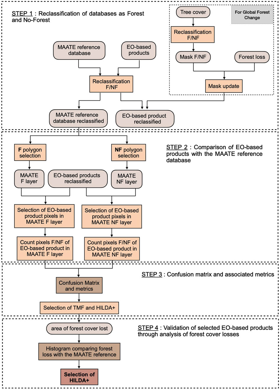
Figure 2. Methodology for selecting one EO-based product. F for Forest, NF for No Forest.

3.2.1 Reclassification of databases as forest/no forest

We classified all the different EO-based products and the MAATE database, used as LULC reference, into two categories: Forest vs No-Forest. The goal is to homogenize the classes, since initially the number of classes is different, so that the products are comparable (Vancutsem et al., 2012; Pérez-Hoyos et al., 2017). For each year, we defined as Forest, all forest categories as initially defined in each product, all other land use categories being defined as No-Forest. Specifically, for GFC, we reclassified the initial Tree Cover (year 2000), considering as Forest pixels the pixel with a tree cover percentage >10% and No-Forest the rest of the pixels. The output is a Forest/No-Forest mask for the year 2000, which is updated for each year by subtracting the tree cover losses for that year, resulting in a reclassified F/NF map for each year. For GLCLUC we consider Forest pixels the pixels with a tree height >5 m. These choices of classifications for the GFC and the GLCLUC are explained by the decision to align as closely as possible with the FAO definition of forest.

3.2.2 Comparison of EO-based products with the MAATE reference databases

From the MAATE LULC reference database, two polygons Forest and No-Forest are selected and extracted, to create two distinct F/NF layers. We then perform an extraction of each pixel for each EO-based product based on the F/NF layers of the MAATE reference database. Each pixel is extracted according to the F or NF layer in which its centroid is located. This step is carried out for the six EO-based product and for each of the available year. Each database therefore retains its spatial resolution.

3.2.3 Confusion matrix and associated metrics

To measure the robustness of the EO-based products, we produced confusion matrix for the 8 years of data (1990, 2000, 2008, 2014, 2016, 2018, 2020, 2022) common to the EO-based product studied and the MAATE product (Congalton and Green, 2008; Olofsson et al., 2014; Phillips et al., 2024). The outputs of the confusion matrices are: True Positive (TP), False Negative (FN), True Negative (TN) and False Positive (FP) (see Supplementary Figure 1). When the pixels in EO-based products contained in MAATE Forest layer are classified as Forest, they are labelled TP, otherwise they are labelled FN. When the pixels in EO-based products contained in MAATE No-Forest layer are classified as No-Forest, they are labelled TN, otherwise they are labelled FP. The outputs of the confusion matrices are used to calculate the associated metrics: (1) The accuracy, (2) the F1-score and (3) the Mathew Correlation Coefficient (MCC).

$\text{Accuracy}=\frac{TP+TN}{TP+TN+FP+FN}$

$\mathrm{F}1-\text{score}=\frac{2·TP}{2·TP+FP+FN}$

$\text{MCC}=\frac{TP·TN-FP·FN}{\sqrt{\left(TP+FP\right)·\left(TP+FN\right)·\left(TN+FP\right)·\left(TN+FN\right)}}$

While Accuracy is commonly used to evaluate the performance of a classification model, the F1-score and MCC metrics provide additional information when classes are unbalanced. In our case, No-Forested areas outweighed Forested areas. However, the F1-score can reach a limit in cases of extreme imbalance, as it does not consider true negatives (TN). The F1-score is defined as the harmonic mean of precision (TP/(TP + FP)) and recall (TP/(TP + FN)), and focuses on the model’s performance with respect to the positive class, ignoring true negatives. As a result, this metric can be biased in the presence of class imbalance, especially when the positive class is underrepresented. In contrast, the MCC incorporates all components of the confusion matrix (TP, TN, FP, FN) into a single correlation-based formula, allowing it to measure the overall consistency between predictions and true labels, regardless of class distribution. Therefore, MCC is more robust to class imbalance and provides a more reliable evaluation of the model’s overall performance, especially in multi-class or highly imbalanced scenarios (Chicco and Jurman, 2020; Luque et al., 2019). The MCC metric is more robust to imbalances. At the end of this step, two databases are selected: HILDA+ and TMF.

3.2.4 Validation of selected EO-based products through analysis of forest cover losses

Confusion matrices were used to validate the spatial distribution of forest cover. The final step was to quantitatively evaluate the remote sensing products selected from the confusion matrices on forest cover loss. Net losses are shown in diagram form. This quantitative comparison between the remote sensing products selected and the MAATE led to the selection of HILDA+. We will analyse the deforestation process with HILDA+, and we will therefore use the definition of Forest provided by HILDA+, which is based on the FAO definition.

3.2.5 Identification of changes in the dynamics of forest cover obtained with HILDA+

In order to identify the changes in forest cover dynamics obtained with HILDA+, we analysed the annual time series expressed as forest area (km²). We applied a local linear regression with a sliding window of 7 years, allowing to estimate the local slope of the forest trajectory at each date. The slope of this regression, expressed in km²/year, is an estimate of the first derivative of the series, i.e., the annual rate of change in forest cover (Verbesselt et al., 2010). It allows the local characterization of the intensity of the loss (more or less strong negative slope) or the relative stability of the cover (slope close to zero). The changes in slope from 1 year to another, obtained by calculating the difference between two successive slopes, correspond to the second derivative of the series. This second derivative provides information on trend variations in the forest trajectory, particularly by identifying accelerations, slowdowns or breaks in deforestation processes (Verbesselt et al., 2010). Years in which this slope change exceeds a predefined threshold (85th percentile) are considered significant breaks in canopy evolution. These breaks were then grouped when they were less than 5 years apart, and the three most marked events were selected. This approach allows for the robust identification of tipping points in forest cover change, taking into account not only the trend but also its inflections. This approach makes it possible to mathematically detect key moments of change in the forest trajectory, whether they are accelerations, slowdowns or trend reversals (Supplementary Figure 2).

4 Results

4.1 Accuracy assessment of the different EO-based products

The metrics associated with the confusion matrix (Figure 3) allow us to analyse accuracy, F1-score and MCC, and to guide the analysis by selecting the best-performing databases. The databases with the highest accuracy are HILDA+ and TMF, with values between 0.75 and 0.82 and between 0.75 and 0.78 respectively. In 2018, HILDA + correctly classified 82% of instances. In contrast, the MODIS database displays the lowest accuracy values, correctly classifying between 40% and 42% of instances over the 2008–2020 period. Accuracy values of all database range between 0.4 and 0.65. The highest F1-score is displayed by HILDA+, varying between 0.61 and 0.64. In contrast, the lowest is displayed by MODIS, which ranges from 0.44 to 0.47. Analysing the MCC metric, we can see that the highest values displayed by HILDA + are between 0.45 and 0.5. TMF also has an MCC close to that of HILDA+, with values between 0.43 and 0.45. Those for MODIS vary between 0.18 and 0.19. The MODIS values show a strong difference between F1-score and MCC, with F1-score values twice as high as MCC values. If the MCC is much lower than the F1-score, this may indicate that the model has a problem with True Negatives or False Positives.

Figure 3

Figure 3. Confusion matrix metrics resulting from the comparison between Forest and No Forest from the MAATE LULC and HILDA+ (black), TMF (dark brown), ESA-CCI (beige), GLCLUC (dark grey), GFC (orange), MODIS (yellow) (a) Accuracy, (b) F1-score, (c) MCC.

Following this initial spatial analysis with confusion matrices based on Forest cover and No-Forest cover, we selected the databases used for a more precise analysis of forest cover gains and losses. The chosen databases are HILDA+, which has a low spatial resolution but goes back to the 1960s, and TMF, which has a more precise spatial resolution but goes back to the 1990s.

4.2 Comparison of deforestation between HILDA+/TMF and MAATE

To validate the two EO-based products selected, we carried out a second analysis that showing the loss of forest cover over the whole period for HILDA+ and TMF compared with MAATE (Figure 4). The gross losses recorded by MAATE are 13,589 km² between 1990 and 2018 on EPSC. The gross losses recorded by HILDA + are 7,905 km² corresponding to 58.2% of the gross losses recorded by MAATE. The gross losses recorded by TMF are 4,890 km² corresponding to 36% of the gross losses recorded by MAATE. Forest cover gains are 2,562 km² according to MAATE. HILDA + observed 27.4% of the gains recorded by MAATE, compared to 66% for TMF. MAATE reports a net loss of 11,028 km². HILDA + reports a net loss of 7,203 km², or 65.3% of the net losses reported by MAATE. TMF reports a net loss of 3,018 km², or 27.4% of the net losses reported by MAATE.

Figure 4

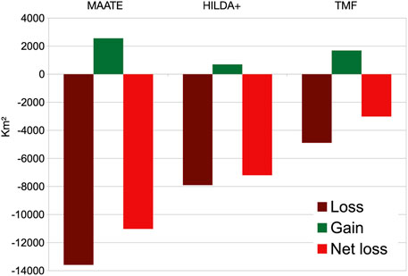
Figure 4. Comparison of gain/loss/net loss between MAATE, HILDA + et TMF over 1990–2018 on EPSC.

Following this analysis, we chose HILDA + to analyse deforestation. Confusion matrices were used to spatially validate HILDA+, which showed good agreement in terms of the spatial distribution of forest cover compared with MAATE. The quantitative comparison of forest cover losses shows that over the period 1990–2018, HILDA + managed to detect more than 65% of the losses reported by MAATE, over a recent period when changes are complex to identify. HILDA + has the advantage of going back to the 1960s. At that date, the uncertainties presented by HILDA + are much smaller than for the recent period. HILDA + can therefore be a good product for obtaining accurate estimates of forest cover and associated losses over the long term. The annual resolution makes it possible to analyse the evolution of the deforestation process and to define phases of deforestation that are more intense than others. From a historical point of view, 1960 marked the beginning of the agrarian reforms that led to the massive displacement of the population and the reorganization of the land, with consequences for the deforestation process.

4.3 Long-term analysis of forest cover evolution of the EPSC over 1960–2019 with HILDA+

We used HILDA + to monitor the evolution of forest cover on the EPSC over 1960–2019 (Figure 5). On the EPSC, between 1960 and 2019, 4 phases were identified in the deforestation process. The first phase between 1960 and 1968 showed a rapid decrease in forest cover from 34,487 km² to 31,714 km², with a net loss of 2,773 km² or 8.04% over 8 years. During the second phase, between 1968 and 1982, forest cover continued to decrease much less rapidly until 1974, when it finally stabilized at about 31,100 km². At the end of the period, in 1982, forest cover had decreased by 9.82% since the 1960s. The third phase between 1982 and 2000, recorded a continuous large loss of forest cover from 31,100 km² to 22,778 km², representing a loss of 8,322 km². At the end of this period, in 2000, forest cover had decreased by 33.95% since the 1960s. The last phase, from 2000 to 2019, exhibited a continuous but less regular and weaker decrease in forest cover than during the previous period, reaching a forest cover of 19,354 km², representing a loss of 3,424 km². Over the last 2 decades, while the trend is still towards a decrease in forest cover, this decrease is 2.4 times less important than over the 18-year period from 1982 to 2000. Over the entire period from 1960 to 2019, forest cover was reduced by 43.88%.

Figure 5

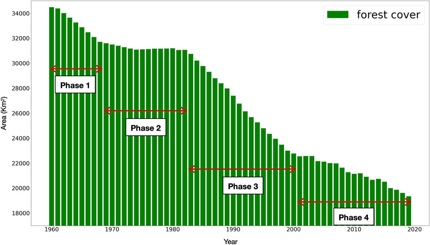
Figure 5. Evolution of forest cover over EPSC from 1960 to 2019 using HILDA+.

Analysis of changes in forest cover at the scale of the EPSC has revealed 4 phases of deforestation. We can then carry out an analysis on the scale of bioclimatic zones to better distinguish the spatio-temporal dynamics of the deforestation process according to forest cover types. The analysis by bioclimatic zones with the HILDA + database (Figure 6) shows that over the entire period between 1960 and 2019, tropical rainforests lost 32% of their area, compared to 54.6% for transition forests and 50.5% for dry tropical forests (Figure 6D). However, while the tropical rain forest and seasonal forests have a similar area, 16,122 km² and 15,938 km² respectively in 1960, dry tropical forests initially have an area almost 6.6 times smaller, with a coverage of 2,413 km² in 1960 (Figure 6D). The dynamics of deforestation differ according to the type of forest considered. There was a net loss of forest cover twice as large in the period 1960–1970 for tropical transition forests with a loss of 2,000 km² at the end of the 1970s against 1,000 km² for tropical rainforests (Figures 6A,B). Deforestation rates remained stable during the 1970s and 1980s and there was almost no deforestation until the early 1980s for dry tropical forests. The period 1980–1990 marks the beginning of a strong deforestation of dry tropical forests with net losses multiplied by three and a loss of 14.3% of forest cover in 10 years (Figure 6C). In this period, the net losses recorded for tropical transition forests are 2.5 times higher than in the previous period and 2 times higher for tropical rain forests. At the end of the 1990s, transition forests lost 30.6% of their area compared to 1960, while tropical rainforests lost only 11.6% of their original area in 1960 (Figures 6A,B). The largest losses for the period 1990–2000 were recorded for tropical rainforests with a net loss multiplied by 2, reaching a loss of 24.6% since the 1960s (Figure 6A). For the last two periods, net loss of forest cover for all bioclimatic zones continues to increase steadily but less rapidly than in the other two periods (Figures 6A–C).

Figure 6

Figure 6. Evolution of forest cover by bioclimatic region outlined in red between 1960 and 2019 according to HILDA+, (A) rain climate, (B) seasonal climate and (C) dry climate. The central graphs show the cumulative loss of forest cover per decade for the three bioclimatic zones. The lower graph (D) shows the area of forest cover in 1960 and 2019 for the three bioclimatic regions.

5 Discussion

5.1 Uncertainties of HILDA+ and TMF

5.1.1 Uncertainties of HILDA + layers

HILDA+ is based on a combination of several remote sensing LULC databases and statistics such as those of the FAO. HILDA + provides annual layers of uncertainty information that express the concordance between the different land cover databases from which HILDA+ is based. Thus, HILDA + provides the mean class area fraction from all available datasets per year to generate per-pixel quality information (Winkler et al., 2021) (Figure 7). The increase in uncertainty over time can be explained by various factors.

Figure 7

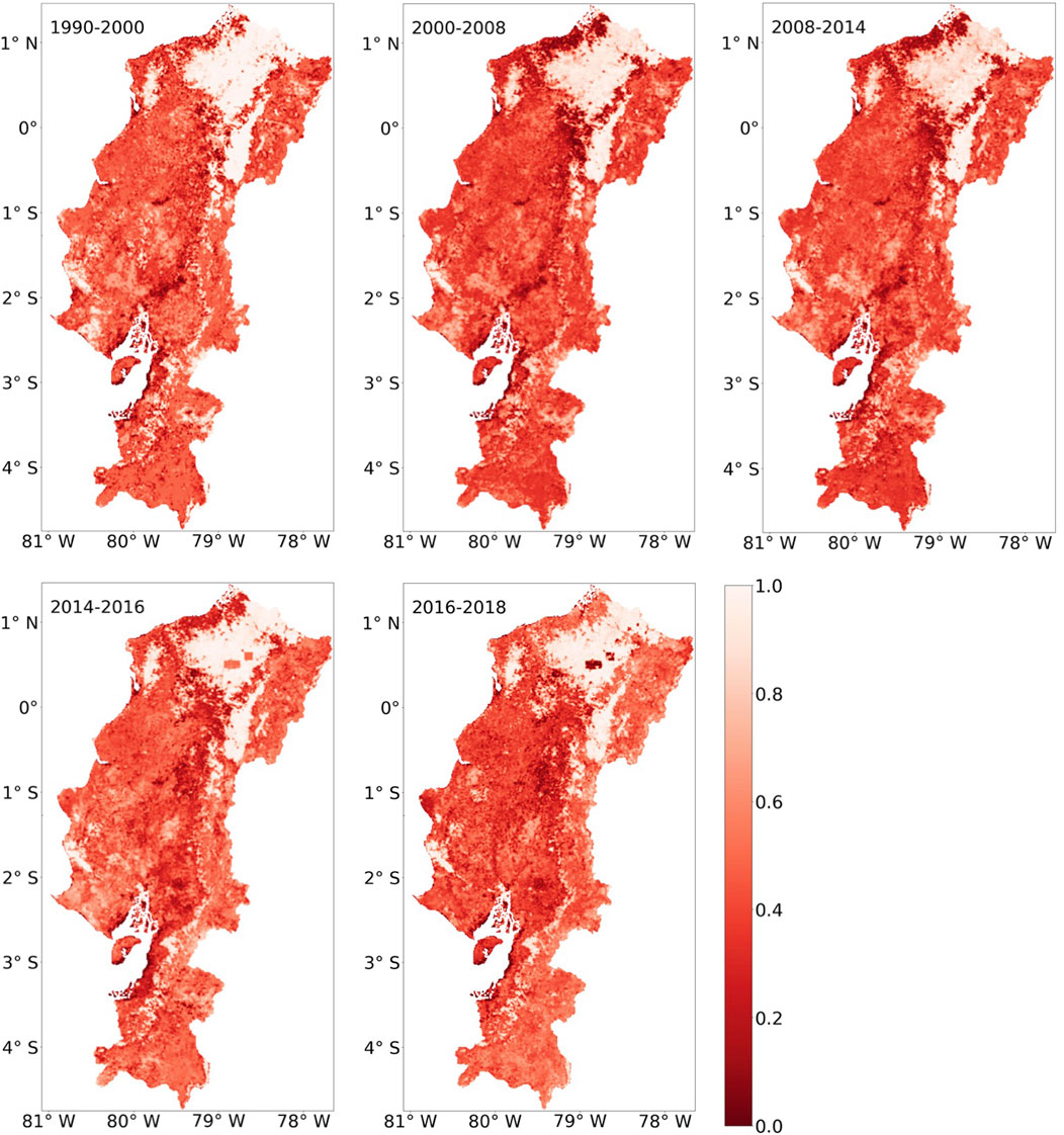
Figure 7. Uncertainty layers provided by HILDA + representing the average surface fraction by land use/land cover category for the different periods used in the validation process.

The increase in the number of datasets used by HILDA + over time has led to higher uncertainty over the recent period. The concordance between all databases is more complicated to obtain when the number of databases is high. Until the 2000s, HILDA+ is based on two or three databases: GLAD UMD VCF available from 1982, Global Human Settlement Layer available for 1975 and 1990, and ESA-CCI Land Cover available from 1992. Since the 2000s, HILDA + has relied on seven databases. In addition to the three databases mentioned above, HILDA + relies on: GLC 2000, Globeland30, Hansen GFC, MODIS MCD12Q1, Ramankutty cropland (Winkler et al., 2021). The multiplication of datasets introduces more variability, potential for errors and increases overall uncertainty. For the earliest periods, few databases are available.

The uncertainty over recent periods can also be explained by the increasing complexity of farming systems and land use dynamics. In recent years, the diversification of agricultural systems has led to a complex mosaic of plots with different uses that land use change models have difficulty in accurately representing. This difficulty, linked to the increasing complexity of landscapes is mentioned by HILDA+, which states that “dataset deviation is larger in agricultural categories cropland and pasture/rangeland. Especially in heterogeneous landscapes, which hold a mix of managed and unmanaged lands, land use/cover class coverage is ambiguous (lower area fractions) and, thus, dataset information deviates” (Winkler et al., 2021).

In addition to the complexity of landscapes, rapid changes in land use related to socio-economic and climatic conditions may explain some of the high uncertainty that occurred mainly during the period 2000–2008. During this period, the country was affected by several crises and economic instability that led to rapid changes in land use. During the same period, extreme weather events such as El Niño and La Niña also affected ecological processes by causing prolonged droughts or floods. These events have had a direct impact on agricultural practices. Adaptation of agricultural practices to cope with these extreme climatic conditions is manifested by rapid and sometimes temporary changes in land use and increase the uncertainty of data for this period. The spatial resolution of HILDA + at 1 km may be inadequate to represent this landscape complexity and increases uncertainty over this period.

Another factor may explain the errors and uncertainties. HILDA+ is constructed from land cover databases produced with optical images that are subject to cloud cover. This aspect is clearly highlighted in the case of the TMF database.

5.1.2 Uncertainty of TMF layers

TMF provides layers representing the number of valid Landsat observations per year. Observations are considered valid when the image is cloud-free, fog-free, sensor artifacts and location issues. EPSC is largely subject to the presence of clouds accounting for the low number of valid observations (Figure 8). Even if the number of valid observations increased with time as new Landsat missions with higher temporal sampling periods were put into orbit, it remained in many locations even in the recent years. For example, in the Province of Manabi, located between the coast of the coastal cordillera in the center of EPSC, over the period 2016–2018, the number of valid observations ranged between 0 and 18 and has an average of 0.71 per year. Areas with several valid observations per year are located above 1,000 m. The low number of useful optical images in coastal areas decreases the reliability of TMF over these areas (Vancutsem et al., 2021).

Figure 8

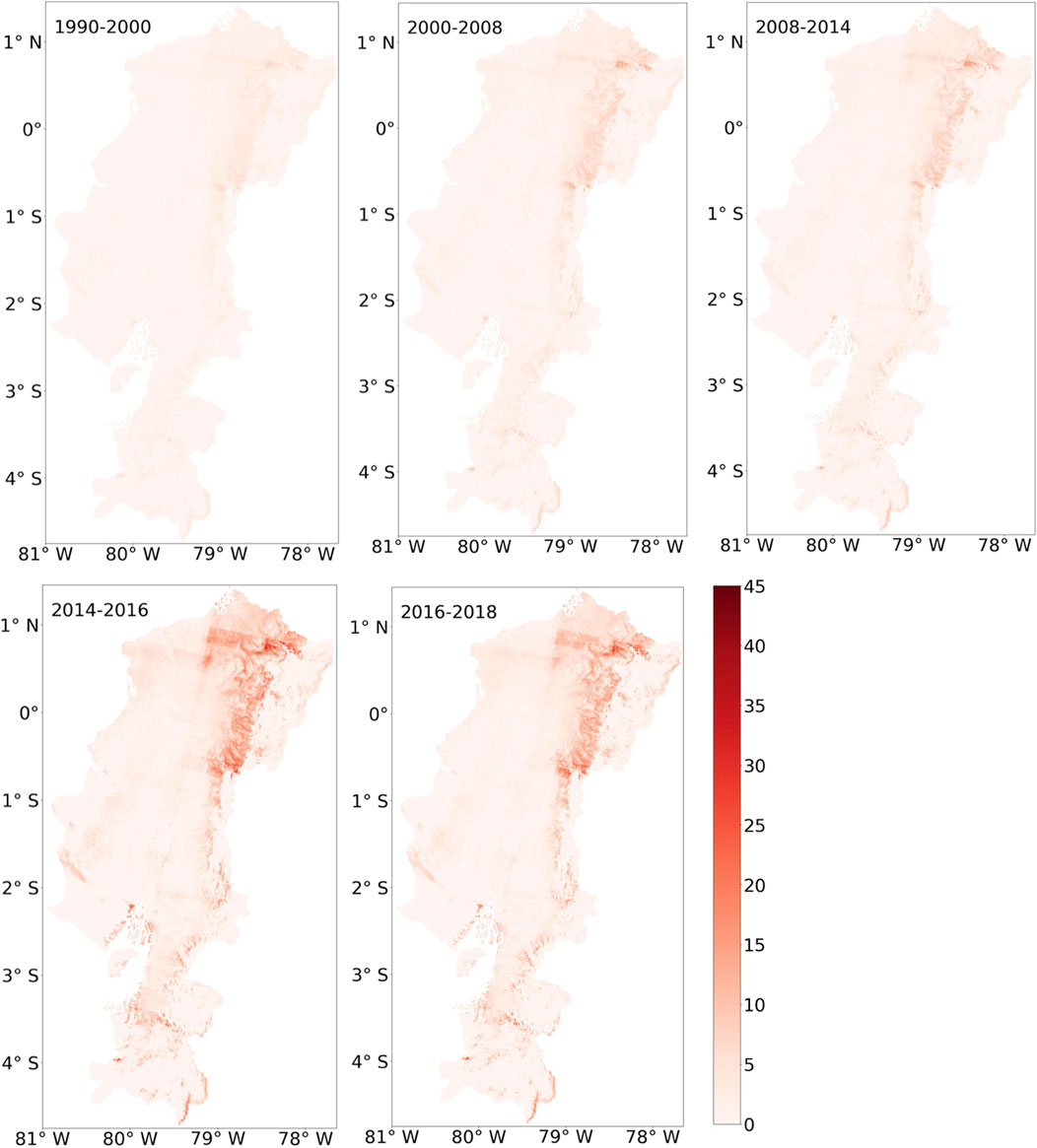
Figure 8. The average number of valid Landsat observations is used to generate TMF LULC per year for the different periods used in the validation process.

5.2 Analysis of the four phases of forest cover evolution

Between 1960 and 2019, the EPSC experienced four periods of deforestation (Figure 5). These four phases can be explained by anthropogenic and climatic factors.

The first phase of deforestation highlighted by HILDA + took place between 1960 and 1968. During this period, the forest cover has been steadily and rapidly decreasing from 34,487 km² to 31,714 km² (Figure 5). Over the whole period, a net loss of 2,773 km² was recorded. The first phase is the consequence of a structural transformation of Ecuadorian society and economy that began in the 1950s, with a shift from a rural and agrarian economy to an urban society and a commercial economy. The banana economy replaces the predominant cocoa crop after the end of World War II (Cabarle et al., 1989) and marks the culmination of the agro-exporter model. This agricultural change, with export agriculture, created a need for new land having land or river access to the ports (Delavaud, 1980) to be directly linked to world markets (Fauroux, 1981).

This evolution of the economic model was accompanied by a demographic boom. The increase in the population of cities during this period caused a need to increase agricultural supply (Salvador Lara, 1995). The increase in population in the Sierra generated pressure on the existing production area. These changes led the state to intervene in the reorganization of production systems to meet the need to increase agricultural supply and encourage the population of the Sierra to colonize the regions of the Costa. The State established a project for restructuring Ecuadorian agriculture that resulted in the agrarian reforms of July 1964 and October 1973. These reforms abolished old colonial inherited production relationships where a few owned most of lands and aimed at a more equitable redistribution allowing landless farmers to own small plots (Fauroux, 1981; Deler, 1987). The objective of the State was to increase productivity and expand the supply of manufactured products (Fauroux, 1981). The migration of landless peasants, especially from the uplands, was an essential factor in the expansion of agricultural borders into the forested areas of the coast (Commander and Peek, 1986). This economic change is encouraged by the Ecuadorian state, which promotes the expansion of agricultural land by granting loans and land to Ecuadorian and foreign entrepreneurs and peasants.

Nevertheless, we found with HILDA + data that in the period 1960–1970, seasonal forests on the central coast are twice as affected as tropical rainforests in the north of the country (Figures 6A,B). This spatial distinction is confirmed by Sierra and Stallings (1998) which explains that this first period of deforestation is concentrated on the central and northern coast and is explained by the fact that the process of deforestation remains limited by an emerging transport network outside the traditional axes: Quito-Guayaquil-Cuenca. At that time, the north of the province of Esmeraldas was still inaccessible (Figure 6A) (Fauroux, 1981; Sierra and Stallings, 1998).

The second phase of deforestation identified with HILDA + corresponds to a period of stabilization of forest cover between 1968 and 1982 over the entire EPSC (Figure 5). The analysis of the losses of forest cover in the three bioclimatic zones shows a stabilization of the forest cover loss over the whole period (Figures 6A–C). This stabilization is explained by several factors. The failure of the State in the restructuring of agriculture has social and economic consequences that affect forest cover, with a slowdown in deforestation and a gradual stabilization of forest cover over the period. This stabilization of the forest cover on the EPSC can also be related to the beginning of the deforestation period in the Amazon basin with the exploitation of oil resources (Southgate and Whitaker, 1992).

The failure of agrarian reforms caused a multidimensional crisis on the coast, with a peasantry revolt that materialized by a phenomenon of invasion of the land which accelerated in 1975, giving rise to clashes between peasants and the police and tensions between employers and workers (Fauroux, 1981). This period of tension slowed the clearing of land on the Pacific coast of Ecuador. This social crisis was compounded by the problem of overproduction of bananas in 1968, which also led to a crisis and massacres in the cities of Guayaquil. These socio-economic phenomena caused deforestation to slow down. The impoverishment of farmers and the failure of agricultural products markets were slowed down by inefficient storage methods and the still little developed ENSO communication links between the different production areas lead to shortages in some places and overproduction of products in others.

Another phenomenon explained a slowdown in deforestation on the coast. During this period, the Oriente began to be coveted for its oil resources, which led to the construction of roads to serve oil production, especially around Nueva-Loja that began in the 1970s (Deler, 1987; Lopez, 2021). Infrastructure development was supporting rapid settlement and agricultural expansion in the Oriente. Between the 1974 and 1982 censuses, 92,700 people settled in the four eastern provinces of Ecuador (Southgate et al., 1991). The 1982 census showed that a relatively small proportion of the labor force found employment in the oil industry and 60% of the economically active population of the region worked in agriculture. Thus, the oil boom of the 1970s caused the share of agricultural products in total exports to fall: in 1964 all agricultural products (bananas, coffee, cocoa) represent 89.2% of the country’s exports, compared with 36.2% in 1976, while oil exports account for 47.8% (Fauroux, 1981).

The third deforestation period runs from 1982 to 2000. There is a continuous large loss of forest cover from 31,100 km² in 1982 to 22,778 km² in 2,000 (Figure 5). Deforestation now affects all bioclimatic zones (Figures 6A–C). By establishing a spatio-temporal differentiation, between 1980 and 1990, we observed greater losses of dry tropical forests and transitions and from the 1990s, the deforestation process moved towards the north of the country, and since 1990, tropical rainforests were the most affected biome by deforestation. Sierra and Stallings (1998) also point to a resumption of deforestation on the Costa. The period of deforestation is due to the development of the road network mainly in the north of the country. On the Costa, construction of new roads began in the 1970s, such as those to access La Tola, at the extreme northwest of the country and later, Borbón and the lower Santiago River. The consequences of these constructions on deforestation are visible only from the 1980s with the extension of the agricultural border to the forests of the north of Esmeraldas. In 1982, almost half of the population of the parish of Borbón was made up of immigrants, compared to 20% in 1978. The number of immigrants in Malimpia Parish tripled between 1978 and 1982 and quadrupled between 1982 and 1990 (Sierra and Stallings, 1998). Then, in the 1980s, new roads were built from the coast inland, following rivers and forest paths (for example, in the parishes of Chontaduro and Chumunde). By the late 1980s, many areas north of Esmeraldas, particularly near the coast, were dominated by settlers. The 1990s marked the beginning of a process of rapid expansion of agriculture on the coast, and mainly in the north, where Esmeraldas became a province that attracted people through the availability of land to produce agricultural products for export (mainly bananas, coffee and cocoa).

The oil economy also had important multiplier effects. Subsequently, oil extraction has created urban and rural jobs with relatively high wages, generating demand for services, food and other commodities produced in the deforested areas. The consequences of the oil economy are the development of regional markets, stimulating the development of a commercial agricultural sector for domestic markets. During this period, there is an expansion of agricultural land on the Costa.

Sierra and Stallings (1998) have highlighted the role of selective timber extraction in north-western Ecuador [for example, heavy woods such as chanul (Humiriastrum sp.) and guayacán (Tabebuia sp.)]. This aspect is also widely discussed by Amelung and Diehl (1992) and Guppy (1984). Nearly 70% of the deforestation that occurred in the forests of the north-west of the EPSC between the 1980s and 1990s can be explained solely by timber extraction (Sierra and Stallings, 1998). In addition to the anthropogenic disturbances described, there were also climatic disturbances during this period, with two major ENSO episodes, in 1982–1983 and 1997–1998, responsible for extremes inundations (França et al., 2020; Quiroz, 1983).

The fourth period of deforestation between 2000 and 2019 is characterized by a slowdown in deforestation compared to the previous period (Figure 5). With HILDA + there was a decrease in forest cover which is 2.5 times less rapid compared to the period 1982–2000. This period of deforestation, which corresponds to the last 20 years, is characterized by a contraction of the agricultural area and a tendency to a decrease in deforestation compared with the previous period, with a significant slowdown in the expansion of agricultural land, a decrease in demand for new agricultural land and an intensification of rural production systems. This is due to much lower population growth rates than in the past and the concentration of the country’s population in dense urban and rural areas. This population concentration was responsible for about 60% of the decrease in deforestation in the Ecuadorian provinces (MAATE, 2017). When the annual growth of urban areas was high (between 2000 and 2008) compared to the 1990s, deforestation was lower. Beyond these social factors, which contributed to the decrease in deforestation, when the country’s economy entered crisis in 1999, deforestation decreased. Thus, the recurrence of El Niño, the fall in oil prices and the financial crisis of 1998–1999 have had a major impact on the national economy and household purchasing power (Ramírez and Ramírez, 2005). The 1998 EL Niño event caused losses equivalent to 14.5% of GDP and the 1998/1999 crisis cost between 25% and 22% of GDP. The fall in oil prices in 1998 aggravated the fiscal crisis, forcing the state to cut public services and transfers. Public social expenditure, which had increased between 1992 and 1996, fell by 37% between 1996 and 1999. This has resulted in an increase in urban poverty, from 19% of households in 1995 to 42% in 1999. In rural areas, it rose from 56% to 77% (Ramírez and Ramírez, 2005). The crisis has been a trigger for a general decline in demand for agricultural products and deforestation. From 2005, once the impact of the crisis and inflation linked to dollarization are under control, we observe a reactivation of deforestation in some regions such as north of Esmeraldas (Figure 6A).

6 Conclusion

The HILDA + database used in this study has the specificity of being based on a combination of Land Use/Land Cover databases from satellite images. This database was selected in two stages. Firstly, six EO-based products were compared with the MAATE reference database using a confusion matrix and associated metrics. At the end of this first stage, two databases were selected: TMF and HILDA+ with maximum overall accuracy of 0.78 and 0.82 respectively. This was followed by a more detailed analysis of forest cover losses and gains. Through the spatial and quantitative validation of HILDA+ with the MAATE reference database, we were able to analyse the evolution of deforestation on the EPSC between 1960 and 2019.

Thanks to the annual temporal resolution of HILDA + we were able to highlight four phases of deforestation over the whole study area. An initial period of intense deforestation from 1960 to 1968, which corresponds to the banana boom, followed by a period of stabilization of forest cover from 1968 to 1982 with the start of oil exploitation in the Amazon basin. The deforestation process is then relaunched until the 2000s, promoted by public policies and globalized trade. The fourth period of deforestation is characterized by a slowdown, related to political and social crises. At a spatial resolution of 1 km, we were able to establish a spatial differentiation of the deforestation process according to the three bioclimatic zones (rain climate, seasonal climate and dry climate), which are not affected during the same phases of deforestation. While tropical rainforests have declined by one-third since the 1960s, dry and seasonal forests lost more than half of their surface area between 1960 and 2019.

One of the limitations of HILDA+ is its 1 km spatial resolution. HILDA+'s spatial resolution is an obstacle to analysing deforestation at a finer scale. To analyse the complex changes in the EPSC landscape more accurately over recent years, we need data at higher spatial resolution. Also, HILDA+ is based on databases that use optical images, subject to cloud cover, which is very important above the EPSC. One possibility is to use radar images to overcome the problem of cloud cover. The use of these data could also make it possible to capture climate disturbances linked to the ENSO phenomenon and the rapid inter-annual changes that affect forest cover. Although the spatial resolution of HILDA+ and the optical data used are limiting factors in capturing the complex and rapid changes in landscapes over the recent period, HILDA + presents itself as a coherent product over the long term, validated with the MAATE reference database and making it possible to analyse changes in forest cover over 6 decades at the scale of the whole the EPSC.

Data availability statement

The original contributions presented in the study are included in the article/Supplementary Material, further inquiries can be directed to the corresponding authors.

Author contributions

VS: Conceptualization, Data curation, Formal Analysis, Funding acquisition, Investigation, Methodology, Project administration, Resources, Software, Supervision, Validation, Visualization, Writing – original draft, Writing – review and editing. FF: Conceptualization, Funding acquisition, Investigation, Methodology, Project administration, Supervision, Writing – review and editing. LB: Conceptualization, Funding acquisition, Investigation, Project administration, Supervision, Writing – review and editing. TC: Writing – review and editing. MP: Conceptualization, Funding acquisition, Investigation, Project administration, Supervision, Writing – review and editing. SR: Writing – review and editing. LH: Formal Analysis, Methodology, Resources, Writing – review and editing. J-PW: Supervision, Writing – review and editing.

Funding

The author(s) declare that financial support was received for the research and/or publication of this article. This study was supported by the MELICERTES project (ANR-22-PEAE-0010) of the French National Research Agency, under the France2030 program and the national PEPR “agroécologie et numérique” program. This study was also supported by the PNTS ReTroForRS.

Conflict of interest

The authors declare that the research was conducted in the absence of any commercial or financial relationships that could be construed as a potential conflict of interest.

The author(s) declared that they were an editorial board member of Frontiers, at the time of submission. This had no impact on the peer review process and the final decision.

Generative AI statement

The author(s) declare that no Generative AI was used in the creation of this manuscript.

Publisher’s note

All claims expressed in this article are solely those of the authors and do not necessarily represent those of their affiliated organizations, or those of the publisher, the editors and the reviewers. Any product that may be evaluated in this article, or claim that may be made by its manufacturer, is not guaranteed or endorsed by the publisher.

Supplementary material

The Supplementary Material for this article can be found online at: https://www.frontiersin.org/articles/10.3389/frsen.2025.1536105/full#supplementary-material

References

Amelung, T., and Diehl, M. (1992). “Deforestation of tropical rain forest,” in Economic causes and impact on development. Germany: Tubingen.

Google Scholar

Anderegg, W. R. L., Berry, J. A., Smith, D. D., Sperry, J. S., Anderegg, L. D. L., and Field, C. B. (2012). The roles of hydraulic and carbon stress in a widespread climate-induced forest die-off. Proc. Natl. Acad. Sci. 109 (1), 233–237. doi:10.1073/pnas.1107891109

PubMed Abstract | CrossRef Full Text | Google Scholar

Armenteras, D., Espelta, J. M., Rodríguez, N., and Retana, J. (2017). Deforestation dynamics and drivers in different forest types in Latin America: three decades of studies (1980–2010). Glob. Environ. Change 46, 139–147. doi:10.1016/j.gloenvcha.2017.09.002

CrossRef Full Text | Google Scholar

Barlow, J., Lennox, G. D., Ferreira, J., Berenguer, E., Lees, A. C., Nally, R. M., et al. (2016). Anthropogenic disturbance in tropical forests can double biodiversity loss from deforestation. Nature 535 (7610), 144–147. doi:10.1038/nature18326

PubMed Abstract | CrossRef Full Text | Google Scholar

Baumann, M., Gasparri, I., Piquer-Rodríguez, M., Gavier Pizarro, G., Griffiths, P., Hostert, P., et al. (2017). Carbon emissions from agricultural expansion and intensification in the Chaco. Glob. Change Biol. 23 (5), 1902–1916. doi:10.1111/gcb.13521

PubMed Abstract | CrossRef Full Text | Google Scholar

Blaschke, L. L., Nian, D., Bathiany, , Ben-Yami, M., Smith, T., Boulton, C. A., et al. (2023). Spatial correlation increase in single-sensor satellite data reveals loss of Amazon rainforest resilience. doi:10.48550/ARXIV.2310.18540

CrossRef Full Text | Google Scholar

Cabarle, B. J., Crespi, M., Dodson, C. H., Luzuriaga, C., Rose, D., and Shores, J. N. (1989). An assessment of biological diversity and tropical forests for Ecuador. USAID-Quito.

Google Scholar

Castillón, F., Rau, P., Bourrel, L., and Frappart, F. (2025). Dynamics and patterns of land cover change in the Piura river basin (peruvian Pacific slope and Coast) in the last two decades. Front. Remote Sens. 6, 1529044. doi:10.3389/frsen.2025.1529044

CrossRef Full Text | Google Scholar

Chazdon, R. L., Brancalion, P. H. S., Laestadius, L., Bennett-Curry, A., Buckingham, K., Kumar, C., et al. (2016). When is a forest a forest? Forest concepts and definitions in the era of forest and landscape restoration. Ambio 45 (5), 538–550. doi:10.1007/s13280-016-0772-y

PubMed Abstract | CrossRef Full Text | Google Scholar

Chicco, D., and Jurman, G. (2020). The advantages of the matthews correlation coefficient (MCC) over F1 score and accuracy in binary classification evaluation. BMC Genomics 21 (1), 6. doi:10.1186/s12864-019-6413-7

PubMed Abstract | CrossRef Full Text | Google Scholar

Commander, S., and Peek, P. (1986). Oil exports, agrarian change and the rural labor process: the Ecuadorian sierra in the 1970s. World Dev. 14 (1), 79–96. doi:10.1016/0305-750X(86)90097-5

CrossRef Full Text | Google Scholar

Congalton, R. G., and Green, K. (2008). Assessing the accuracy of remotely sensed data: principles and practices, 2nd Edn. Boca Raton, FL: CRC Press. doi:10.1201/9781420055139

CrossRef Full Text | Google Scholar

Daily, G. R. (1998). Nature’s services: societal dependence on natural ecosystems. Environ. Values 7 (3), 365–367.

Google Scholar

Delavaud, A. (1980). ‘From colonization to agricultural development: the case of coastal Ecuador’.

Google Scholar

Deler, J.-P. (1987). “Review of Loja, une province de l’Equateur, de l’isolement à l’intégration,” in Cahiers du monde hispanique et luso-brésilien, 49 169–172.

Google Scholar

Diertl, K.-H. (2010). Pflanzendiversität entlang eines Höhengradienten in den Anden Südecuadors. Erlangen.

Google Scholar

Erazo, B., Bourrel, L., Frappart, F., Chimborazo, O., Labat, D., Dominguez-Granda, L., et al. (2018). Validation of satellite estimates (tropical rainfall measuring mission, TRMM) for rainfall variability over the Pacific slope and Coast of Ecuador. Water 10 (2), 213. doi:10.3390/w10020213

CrossRef Full Text | Google Scholar

Eva, H. D., Achard, F., Beuchle, R., De Miranda, E., Carboni, S., Seliger, R., et al. (2012). Forest cover changes in tropical south and central America from 1990 to 2005 and related carbon emissions and removals. Remote Sens. 4 (5), 1369–1391. doi:10.3390/rs4051369

CrossRef Full Text | Google Scholar

Fauroux, E. (1981). ‘Equateur: les lendemains d’une réforme agraire’.

Google Scholar

Fehlenberg, V., Baumann, M., Gasparri, N. I., Piquer-Rodriguez, M., Gavier-Pizarro, G., and Kuemmerle, T. (2017). The role of soybean production as an underlying driver of deforestation in the south American Chaco. Glob. Environ. Change 45, 24–34. doi:10.1016/j.gloenvcha.2017.05.001

CrossRef Full Text | Google Scholar

Ferrer Velasco, R., Lippe, M., Tamayo, F., Mfuni, T., Sales-Come, R., Mangabat, C., et al. (2022). Towards accurate mapping of forest in tropical landscapes: a comparison of datasets on how forest transition matters. Remote Sens. Environ. 274, 112997. doi:10.1016/j.rse.2022.112997

CrossRef Full Text | Google Scholar

França, F. M., Benkwitt, C. E., Peralta, G., Robinson, J. P. W., Graham, N. A. J., Tylianakis, J. M., et al. (2020). Climatic and local stressor interactions threaten tropical forests and coral reefs. Philosophical Trans. R. Soc. B Biol. Sci. 375 (1794), 20190116. doi:10.1098/rstb.2019.0116

PubMed Abstract | CrossRef Full Text | Google Scholar

García-Nieto, A. P., García-Llorente, M., Iniesta-Arandia, I., and Martín-López, B. (2013). Mapping forest ecosystem services: from providing units to beneficiaries. Ecosyst. Serv. 4, 126–138. doi:10.1016/j.ecoser.2013.03.003

CrossRef Full Text | Google Scholar

Giam, X. (2017). Global biodiversity loss from tropical deforestation. Proc. Natl. Acad. Sci. 114 (23), 5775–5777. doi:10.1073/pnas.1706264114

PubMed Abstract | CrossRef Full Text | Google Scholar

Goetz, S. J., Hansen, M., Houghton, R. A., Walker, W., Laporte, N., and Busch, J. (2015). Measurement and monitoring needs, capabilities and potential for addressing reduced emissions from deforestation and forest degradation under REDD+. Environ. Res. Lett. 10 (12), 123001. doi:10.1088/1748-9326/10/12/123001

CrossRef Full Text | Google Scholar

González-Jaramillo, V., Fries, A., Rollenbeck, R., Paladines, J., Oñate-Valdivieso, F., and Bendix, J. (2016). Assessment of deforestation during the last decades in Ecuador using NOAA-AVHRR satellite data. Erdkunde, 217–235. doi:10.3112/erdkunde.2016.03.02

CrossRef Full Text | Google Scholar

Graesser, J., Stanimirova, R., Tarrio, K., Copati, E. J., Volante, J. N., Verón, S. R., et al. (2022). Temporally-consistent annual land cover from landsat time series in the southern cone of South America. Remote Sens. 14 (16), 4005. doi:10.3390/rs14164005

CrossRef Full Text | Google Scholar

Guppy, N. (1984). Tropical deforestation. A global view, 928–965.

CrossRef Full Text | Google Scholar

Hansen, M. C., Potapov, P. V., Moore, R., Hancher, M., Turubanova, S. A., Tyukavina, A., et al. (2013). High-resolution global maps of 21st-Century forest cover change. Science 342 (6160), 850–853. doi:10.1126/science.1244693

PubMed Abstract | CrossRef Full Text | Google Scholar

Juarez, H., Pradel, W., Navarrete, C., Gutiérrez, D., Hualla, V., Vanegas, M., et al. (2024). Underlying drivers of deforestation in the Peruvian Amazon and the highland region of the Andes. Int. Potato Cent. doi:10.4160/cip.2024.12.005

CrossRef Full Text | Google Scholar

Kleemann, J., Zamora, C., Villacis-Chiluisa, A. B., Cuenca, P., Koo, H., Noh, J. K., et al. (2022). Deforestation in Continental Ecuador with a focus on protected areas. Land 11 (2), 268. doi:10.3390/land11020268

CrossRef Full Text | Google Scholar

Krieger, D. (2001). The economic value of forest ecosystem services: a review. Washington, DC: The Wilderness Society.

Google Scholar

Lopez, C. (2021). Sur la corde raide: rente pétrolière et développement en Équateur (1972-2017). Rev. la régulation 31. doi:10.4000/regulation.20462

CrossRef Full Text | Google Scholar

Luque, A., Carrasco, A., Martín, A., and de las Heras, A. (2019). The impact of class imbalance in classification performance metrics based on the binary confusion matrix. Pattern Recognit. 91, 216–231. doi:10.1016/j.patcog.2019.02.023

CrossRef Full Text | Google Scholar

MAATE (Ministerio del Ambiente) (2017). Deforestación del Ecuador continental periodo 2014-2016.

Google Scholar

Matthews, R. B., van Noordwijk, M., Lambin, E., Meyfroidt, P., Gupta, J., Verchot, L., et al. (2014). Implementing REDD+ (reducing emissions from deforestation and degradation): evidence on governance, evaluation and impacts from the REDD-ALERT project. Mitig. Adapt. Strategies Glob. Change 19 (6), 907–925. doi:10.1007/s11027-014-9578-z

CrossRef Full Text | Google Scholar

Mosandl, R., Günter, S., Stimm, B., and Weber, M. (2008). “Ecuador suffers the highest deforestation rate in South America,” in Gradients in a tropical Mountain ecosystem of Ecuador Ecological Studies. Editor E. Beck, J. Bendix, I. Kottke, F. Makeschin, and R. Mosandl, (Berlin, Heidelberg: Springer Berlin Heidelberg), 37–40. doi:10.1007/978-3-540-73526-7_4

CrossRef Full Text | Google Scholar

Móstiga, M., Armenteras, D., Vayreda, J., and Retana, J. (2024). Two decades of accelerated deforestation in Peruvian forests: a national and regional analysis (2000–2020). Reg. Environ. Change 24 (2), 42. doi:10.1007/s10113-024-02189-5

CrossRef Full Text | Google Scholar

Myers, N. (1988). Threatened biotas: “hot spots” in tropical forests. Environ. 8 (3), 187–208. doi:10.1007/bf02240252

PubMed Abstract | CrossRef Full Text | Google Scholar

Neves, A. K., Körting, T. S., Fonseca, L. M. G., and Escada, M. I. S. (2020). Assessment of TerraClass and MapBiomas data on legend and map agreement for the Brazilian amazon biome. Acta Amaz. 50 (2), 170–182. doi:10.1590/1809-4392201900981

CrossRef Full Text | Google Scholar

Ochoa-Cueva, P., Fries, A., Montesinos, P., Rodríguez-Díaz, J. A., and Boll, J. (2015). Spatial estimation of soil erosion risk by land-Cover change in the andes OF southern Ecuador. Land Degrad. and Dev. 26 (6), 565–573. doi:10.1002/ldr.2219

CrossRef Full Text | Google Scholar

Olofsson, P., Foody, G. M., Herold, M., Stehman, S. V., Woodcock, C. E., and Wulder, M. A. (2014). Good practices for estimating area and assessing accuracy of land change. Remote Sens. Environ. 148, 42–57. doi:10.1016/j.rse.2014.02.015

CrossRef Full Text | Google Scholar

Ometto, J. P., Sousa-Neto, E. R., and Tejada, G. (2016). “Land use, land cover and land use change in the Brazilian amazon (1960–2013),” in Interactions between biosphere, atmosphere and human land use in the amazon basin. Editors L. Nagy, B. R. Forsberg, and P. Artaxo (Berlin, Heidelberg: Springer Berlin Heidelberg), 369–383. doi:10.1007/978-3-662-49902-3_15

CrossRef Full Text | Google Scholar

Pérez-Hoyos, A., Rembold, F., Kerdiles, H., and Gallego, J. (2017). Comparison of global land cover datasets for cropland monitoring. Remote Sens. 9 (11), 1118. doi:10.3390/rs9111118

CrossRef Full Text | Google Scholar

Phillips, G., Teixeira, H., Kelly, M. G., Salas Herrero, F., Várbíró, G., Lyche Solheim, A., et al. (2024). Setting nutrient boundaries to protect aquatic communities: the importance of comparing observed and predicted classifications using measures derived from a confusion matrix. Sci. Total Environ. 912, 168872. doi:10.1016/j.scitotenv.2023.168872

PubMed Abstract | CrossRef Full Text | Google Scholar

Potapov, P., Hansen, M. C., Pickens, A., Hernandez-Serna, A., Tyukavina, A., Turubanova, S., et al. (2022). The global 2000-2020 land cover and land use change dataset derived from the landsat archive: first results. Front. Remote Sens. 3, 856903. doi:10.3389/frsen.2022.856903

CrossRef Full Text | Google Scholar

Quiroz, R. S. (1983). The climate of the “El Niño” winter of 1982–83—A season of extraordinary climatic anomalies. Mon. Weather Rev. 111 (8), 1685–1706. doi:10.1175/1520-0493(1983)111<1685:TCOTNW>2.0.CO;2

CrossRef Full Text | Google Scholar

Ramírez, F., and Ramírez, J. (2005). La estampida migratoria ecuatoriana: crisis, redes transnacionales y repertorios de acción migratoria’, Centro de Investigaciones CIUDAD. Quito, Ecuador. Available online at: https://digitalrepository.unm.edu/abya_yala/406.

Google Scholar

Richter, M. (2003). Using epiphytes and soil temperatures for eco-climatic interpretations in southern Ecuador. Erdkunde 57 (3), 161–181. doi:10.3112/erdkunde.2003.03.01

CrossRef Full Text | Google Scholar

Rivas, C. A., Guerrero-Casado, J., and Navarro-Cerillo, R. M. (2021). Deforestation and fragmentation trends of seasonal dry tropical forest in Ecuador: impact on conservation. For. Ecosyst. 8 (1), 46. doi:10.1186/s40663-021-00329-5

CrossRef Full Text | Google Scholar

Rivas, C. A., Guerrero-Casado, J., and Navarro-Cerrillo, R. M. (2024). Functional connectivity across dominant forest ecosystems in Ecuador: a major challenge for a country with a high deforestation rate. J. Nat. Conservation 78, 126549. doi:10.1016/j.jnc.2023.126549

CrossRef Full Text | Google Scholar

Rodríguez-Echeverry, J. (2023). Extensification of agricultural land-use generates severe effects on the critically endangered inter-andean dry forest in the Ecuadorian andean landscape. J. Landsc. Ecol. 16 (3), 132–148. doi:10.2478/jlecol-2023-0020

CrossRef Full Text | Google Scholar

Romero-Muñoz, A., Benítez-López, A., Zurell, D., Baumann, M., Camino, M., Decarre, J., et al. (2020). Increasing synergistic effects of habitat destruction and hunting on mammals over three decades in the gran Chaco. Ecography 43 (7), 954–966. doi:10.1111/ecog.05053

CrossRef Full Text | Google Scholar

Salvador Lara, J. (1995). in Breve historia contemporánea del Ecuador (México: Fondo de Cultura Económica), 1.

Google Scholar

Scholze, M., Knorr, W., Arnell, N. W., and Prentice, I. C. (2006). A climate-change risk analysis for world ecosystems. Proc. Natl. Acad. Sci. 103 (35), 13116–13120. doi:10.1073/pnas.0601816103

PubMed Abstract | CrossRef Full Text | Google Scholar

Sierra, R., and Stallings, J. (1998). The dynamics and social organization of tropical deforestation in northwest Ecuador, 1983-1995. Hum. Ecol. 26 (1), 135–161. doi:10.1023/A:1018753018631

CrossRef Full Text | Google Scholar

Sierra, R., Calva, O., and Guevara, A. (2021). “La Deforestación en el Ecuador, 1990-2018. Factores promotores y tendencias recientes,” in Ministerio de Ambiente y Agua del Ecuador, Ministerio de Agricultura del Ecuador, en el marco de la implementación del Programa Integral Amazónico de Conservación de Bosques y Producción Sostenible.

Google Scholar

Southgate, D., and Whitaker, M. (1992). Promoting resource degradation in Latin America: tropical deforestation, soil erosion, and coastal ecosystem disturbance in Ecuador. Econ. Dev. Cult. Change 40 (4), 787–807. doi:10.1086/451977

CrossRef Full Text | Google Scholar

Southgate, D., Sierra, R., and Brown, L. (1991). The causes of tropical deforestation in Ecuador: a statistical analysis. World Dev. 19 (9), 1145–1151. doi:10.1016/0305-750x(91)90063-n

CrossRef Full Text | Google Scholar

Souza, C. M., Z. Shimbo, J., Rosa, M. R., Parente, L. L., A. Alencar, A., Rudorff, B. F. T., et al. (2020). Reconstructing three decades of land use and land cover changes in Brazilian biomes with landsat archive and Earth engine. Remote Sens. 12 (17), 2735. doi:10.3390/rs12172735

CrossRef Full Text | Google Scholar

Tapia-Armijos, M. F., Homeier, J., Espinosa, C. I., Leuschner, C., and de la Cruz, M. (2015). “Deforestation and forest fragmentation in south Ecuador since the 1970s – losing a hotspot of biodiversity,”. Editor C. N. Jenkins, 10, e0133701. doi:10.1371/journal.pone.0133701PLOS ONE9

CrossRef Full Text | Google Scholar

UN Environment Programme (UNEP) and Food and Agriculture Organization of the United Nations (FAO) (2020). The state of the world’s forests: forests, biodiversity and people. Available online at: https://www.unep.org/resources/state-worlds-forests-forests-biodiversity-and-people (Accessed September 19, 2024).

Google Scholar

Vancutsem, C., Marinho, E., Kayitakire, F., See, L., and Fritz, S. (2012). Harmonizing and combining existing land cover/land use datasets for cropland area monitoring at the African Continental scale. Remote Sens. 5 (1), 19–41. doi:10.3390/rs5010019

CrossRef Full Text | Google Scholar

Vancutsem, C., Achard, F., Pekel, J. F., Vieilledent, G., Carboni, S., Simonetti, D., et al. (2021). Long-term (1990–2019) monitoring of forest cover changes in the humid tropics. Sci. Adv. 7 (10), eabe1603. doi:10.1126/sciadv.abe1603

PubMed Abstract | CrossRef Full Text | Google Scholar

Verbesselt, J., Hyndman, R., Newnham, G., and Culvenor, D. (2010). Detecting trend and seasonal changes in satellite image time series. Remote Sens. Environ. 114 (1), 106–115. doi:10.1016/j.rse.2009.08.014

CrossRef Full Text | Google Scholar

Vicente-Serrano, S. M., Aguilar, E., Martínez, R., Martín-Hernández, N., Azorin-Molina, C., Sanchez-Lorenzo, A., et al. (2017). The complex influence of ENSO on droughts in Ecuador. Clim. Dyn. 48 (1–2), 405–427. doi:10.1007/s00382-016-3082-y

CrossRef Full Text | Google Scholar

Wagner, F. H., Dalagnol, R., Silva-Junior, C. H., Carter, G., Ritz, A. L., Hirye, M. C., et al. (2022). Mapping tropical forest cover and deforestation with planet NICFI satellite images and deep learning in Mato Grosso state (brazil) from 2015 to 2021. doi:10.48550/ARXIV.2211.09806

CrossRef Full Text | Google Scholar

T. C. Whitmore, and J. A. Sayer (1992). Tropical deforestation and species extinction (London: Chapman and Hall (The IUCN forest conservation programme), 6.

Google Scholar

Winkler, K., Fuchs, R., Rounsevell, M., and Herold, M. (2021). Global land use changes are four times greater than previously estimated. Nat. Commun. 12 (1), 2501. doi:10.1038/s41467-021-22702-2

PubMed Abstract | CrossRef Full Text | Google Scholar