Performance of segmentation (watershed and meanshift) and image transformation (MNF-laplacian filter) methods for extracting complex coastlines from Pleiades images: the case of the Kerkena archipelago, Tunisia

With the ongoing surge in global coastal development, understanding shoreline dynamics has become a critical issue, given the inherent vulnerability of coastal fringes to significant mobility. Developing tools to support the sustainable management and future planning of these areas requires a robust comprehension of their dynamic behavior. Monitoring shoreline changes through coastline extraction using remote sensing is vital for quantifying the diachronic evolution of shorelines. However, the accuracy of coastline extraction methods can be hindered by various factors, including the quality of geospatial data, the characteristics of the study area, and the adequacy of pre-processing techniques applied. This study evaluates the performance of different coastline extraction methods based on the segmentation (Watershed and Meanshift) and transformation and discrimination (MNF-Laplacian filter) of very high spatial resolution Pléiades images resampled to 0.5 m. This evaluation of the performance of the automatic extraction methods was carried out by comparison with manually Digitized coastlines across different types of coastlines, a methodology that could be applied to other study areas with similar characteristics. The analysis is based on the mean distances and mean differences of the statistics obtained from Digital Shoreline Analysis System with Shoreline Change Envelope Net Shoreline Movement and End Point Rate indices, which quantify the variations in the reference line detected by each method as well as the diachronic changes in the shoreline over 10 years (2012–2022). The results show that the extraction method based on the WaterShed algorithm is the most accurate compared with coastlines obtained by manual extraction. It enables the shoreline to be detected perfectly on developed coasts and sandy coasts. On cliffs, the MeanShift and Minimum Noise Fraction (Minimal Noise Fraction)-Laplacian filter algorithms perform better. Detecting the coastline on cliffs is complex, due to the shadow of the cliffs caused by the sensor’s acquisition angle, and the over-segmentation of the images. The method based on the MNF Laplacian filter combination performed best, with 98.8% of coastline extracted. Taking into account the coastline extracted by the best-performing method for each type of coastline, we could determine an average retreat of the shoreline of −0.33 m/year over 10 years.

1 Introduction

The shoreline is an area characterised by ‘permanent and particularly rapid mobility on a geological time scale, but also on a human time scale’ (Maur-Férec et al., 2004; Anthony, 2008). This environment, whose morphology is shaped by fluctuations in the coastline, is becoming increasingly sought after. For more than a century, human occupation has been intensifying, with increasing coastal development (Amar, 2010; Gustave, 2022). Yet these human settlements are becoming increasingly vulnerable to phenomena related to climate change (increased frequency of storms, sea-level rise). In this context, managing the risk of coastal erosion is becoming a major challenge, and requires considering the evolution of the shoreline dynamics.

In recent years, monitoring changes in the coastline has been widely discussed (Niang-Diop, 1995; Oueslati, 1995a; Paskoff, 2004; Juigner et al., 2012; Etienne, 2014; Thior et al., 2021; Diatta et al., 2022; Gadal et al., 2023a), mainly with a view to managing these vulnerable areas. In fact, geospatial data enables diachronic monitoring of coastal areas and provides information on territorial and environmental dynamics. The availability of such data also makes it possible to take stock of these dynamics and quantify measures of shoreline change. Shoreline detection techniques, which initially focused on visual interpretation, have increasingly turned towards automatic methods that can be reproduced elsewhere (Louati et al., 2014; Bengoufa et al., 2021; Gadal et al., 2023a; Boussetta et al., 2023). Monitoring coastline movement using geospatial data is therefore part of a process to produce reliable results. However, various processing methods can be used to obtain similar results.

The aim of this article is to evaluate the performance of automatic coastline extraction methods on high-resolution images acquired by the Pléiades satellite. Two methods were evaluated: (i) the first one is based on image transformation using a combination of the MNF and Laplacian filter algorithms and (ii) the second one is based on image segmentation using the WaterShed and MeanShift algorithms. The performance of the different coastline extraction methods was assessed in terms of the mean distance and the mean difference in statistics between manually Digitized and automatically extracted coastlines from two Pléiades images acquired in March 2012 and February 2022. The advantage of these images lies in their resolution of 0.7 m and their spectral characteristics (4 spectral bands and a panchromatic band), which enable good detection of geographical objects (water, dry sand, wet sand, urban development, cliff edge, etc.).

2 Study area

The Kerkena archipelago lies to the south-east of the Tunisian coastline, on the north part of the Gulf of Gabès, 20 km off the coast of Sfax. Approximately 35 km long and 10 km wide, it comprises a group of twelve islets and two main islands: Gharbi (48 km²) and Chergui (99 km²). These two islands cover around 150 km², a large part of which is occupied by sebkhas (marshes–lands that are periodically flooded and unsuitable for farming due to their salinity). This location in the Gulf of Gabès is conducive to complex hydrodynamic phenomena, with a convergence of currents of Atlantic origin, entering through the Chebba Strait, and those of Levantine origin, entering through the Sfax Strait (Ben Mustapha, 2007). The archipelago is subject to significant tidal variation, as is the rest of the Gulf of Gabès, to which it belongs. With a coastline 181 km long, the archipelago’s coastal zone is mainly characterised by the presence of cliffs or micro-cliffs cut into various substrates, large salt marshes favoured by an important tide and limited sandy shorelines. The western side, where the archaeological site of Borj El H’ssar and the tourist facilities in the Sidi Frej area are located, is more exposed to the prevailing winds and sea currents, while the eastern sector of the archipelago is more protected from these hydrodynamic agents (Figure 1). The exposure of this sector to the prevailing winds and the lithological complexity, with alternating hard rock and loose sediment, favour differential erosion, which is justified by the presence of a rugged profile, unlike the eastern sector, which has a straight shape. The study area covers the sector from Karaba beach to the tourist sector of Sidi Frej, including the archaeological site of Borj El H’ssar (Figure 1).

Figure 1

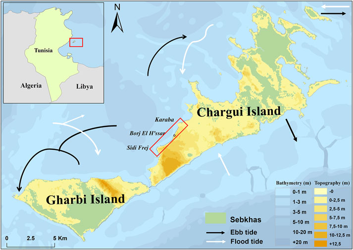
Figure 1. Localization of the studied area on a topographic map of the Kerkena archipelago with tidal currents and bathymetry, Diatta 2024 after Etienne, 2014, drawing N. Basuau ©Projet Kerkena (K. Schörle and A. Drine).

3 Methods and datasets

3.1 Satellite data characteristics and pre-processing protocols

Two satellite images were used in order to obtain the results presented here. Ideally, more satellite images should be used over longer and regular chronological periods in order to strengthen the protocol, but only one archival image from 2012 of the entire case study area suited the purpose of this study. The 2012 image was retrieved from the DINAMIS¹ archive catalogue; the 2022 image was obtained through satellite tasking. Pléiades is a near-polar orbiting satellite offering very high-resolution imagery, with four 2.8 m spectral bands (blue, green, red and near infrared) and a 0.7 m panchromatic band. After pansharpening, we obtain a colour image with 0.5 m after resampling at ground level using the Bayesian algorithm on the open-access application OTB (Orfeo ToolBox). This high resolution enables a good detection and identification of geographical objects. The original images were ordered as ‘Primary’, i.e., in the sensor geometry. Orthorectification is therefore the geometric correction and georeferencement stages that enable to move from the ‘Primary’ images to the ortho-images directly usable in GIS software (Figure 2). The process involves using the DIMAP (Digital Image Map) file associated with the spectral bands and assigning it the exact projection system corresponding to the study area (WGS 84 UTM Zone 32N). Orthorectification, pansharpening and resampling were carried out on the OTB. The accuracy of the georeference performed by the orthorectification process was checked against reference data, such as the Google satellite imagery used for this study.

Figure 2

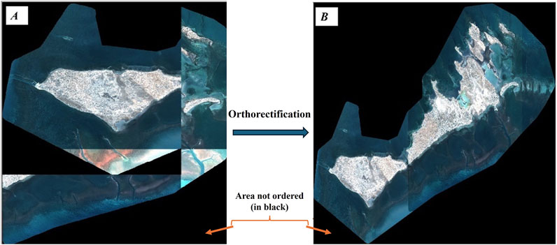
Figure 2. 2022 «PRIMARY» image in the original geometry of the satellite Pléiades sensors (A) and the orthorectified and so georeferenced image in QGIS (B). Pléiades^© CNES (2022), distribution AIRBUS DS.

After orthorectification and resampling, the coastline was automatically extracted and compared with a manual extraction.

3.2 Coastline extraction methodology

Two automatic coastline extraction methods have been applied (Figure 3). The first is based on image segmentation using the MeanShift and WaterShed algorithms. The second is based on image transformation using the MNF algorithm, followed by discrimination of new images using a 7 × 7 convolution Laplacian filter. These methods were compared with the one based on digitizing the coastline using photointerpretation.

Figure 3

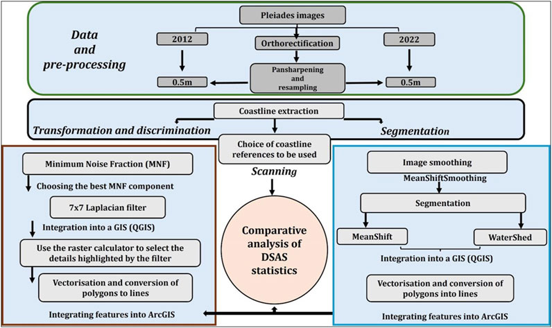
Figure 3. Diagram summarizing the methodology used.

3.2.1 Digitization of the coastline

Digitization of the reference line requires prior identification of coastline position markers. These markers are easily identifiable on Pléiades images due to their high resolution. Three markers were taken into account for this study: 1) the cliff boundary, which is the point at which waves undercut the shoreline, 2) the boundary of urban development, with buildings in the foreground, which is also the point at which waves undercut the shoreline, and 3) the wetting boundary, i.e., the boundary between dry and wet sand on the shoreline. The morphological characteristics of the area and the objectives of the study guided the choice of these three indicators. Once we had identified the indicators of the position of the coastline, we proceeded to digitize it. This was done using ArcGIS at a scale of 1:50 (allowing a good distinction of pixel boundaries) by following the shoreline markers on the 2012 and 2022 images. However, due to the angle of incidence of the Pléiades satellite sensors and the characteristics of the study area (shading created by cliffs), the digitization of the position of the coastline is disrupted on certain sections of the coastline studied. With this in mind, it is important to determine the margin of error of the digitization. This is calculated using the following formula (Gadal et al., 2023b):

$En=\sqrt{Egeore{f}^2+Edi{g}^2}$

En is the margin of error for digitizing the coastline, Egeoref is the margin of error for georeferencing, which is obtained by re-aligning the image with the reference data (Google satellite imagery), and Edig is the margin of error linked to the uncertainty in digitizing the coastline. The latter depends on visibility of the coastline, the experience, the knowledge of the study area and must be included at the discretion of the operator responsible for Digitization. For the 2022 image, the accuracy of the Digitization around the Borj El H’ssar site has been improved by the use of DGPS points taken in the field during a Tunisian-French mission in 2022. The margin of error for Digitization is therefore 0.27 m for the 2012 image and 0.23 m for 2022.

$\text{En\hspace{0.17em}}\left(2012\right)=\sqrt{{0.15}^2+{0.23}^2}=0.27\mathrm{m}$

$\text{En\hspace{0.17em}}\left(2022\right)=\sqrt{{0.13}^2+{0.20}^2}=0.23\mathrm{m}$

3.2.2 Automatic coastline extraction using image segmentation

The coastline was extracted from the image segmentation using the WaterShed algorithm and the MeanShift algorithm. WaterShed uses the spectral information of the image translated into shades of grey to group pixels with the same spectral characteristics. It considers a grayscale image as a topographical relief where each pixel has an altitude, from which we simulate flooding and calculate the gradient of the image. The areas of high intensity form the hilltops, while the low intensities form the valleys (Hugueny, 2014). Watershed lines are then created to prevent merging when two valleys of different intensities meet (Beucher, 1992). Given that the coastline limits chosen for this study are the limit of the wetting zone and the limit of the cliff and/or developments, which in this case correspond to the point of water undercutting at high tide, this segmentation makes it possible to detect the contours of the geographical objects that characterise the coastal zone studied. The MeanShift algorithm, on the other hand, is based on an iterative gradient ascent procedure for unsupervised clustering and/or mode determination (Zegaoua, 2012). It relies not only on information about individual pixel values, but also on contours: texture, shape and topology (Bengoufa et al., 2021). The advantage of this algorithm lies in the fact that it improves images by reducing noise and improving the sharpness of contours. MeanShift transforms the image by considering a colour space in which each cluster corresponds to segmented regions of the original image (Beck et al., 2018).

• In order to optimize our results when applying segmentation, we carried out a spatial initialization of the image. This removes low contrast minima and highlights pixels with a high probability of belonging to the same class. The result is a classified image with pixel contrasts in the form of classes based on the spectral characteristics of the objects. These classes are considered as relief by the WaterShed algorithm for the definition of valleys (classes or objects) and as clusters by the MeanShift algorithm for the definition of regions. Smoothing is then used to avoid over-segmentation of the image as far as possible. The Meanshift Smoothing algorithm was used to perform this smoothing. After testing different gradients coefficients (0; 0.5; 0.75; 1), we chose the 0.5 coefficient for this study (Figure 4. 1). This produces a more uniform image and good segmentation.

• The smoothing results were then segmented, firstly using the WaterShed algorithm and secondly using the MeanShift algorithm (Figure 4. 2).

• We then vectorized the segmented output (Figure 4 3 and A), which was then converted into simplified lines.

• Finally, we extracted the line corresponding to the chosen reference (Figure 4. B, yellow line).

Figure 4

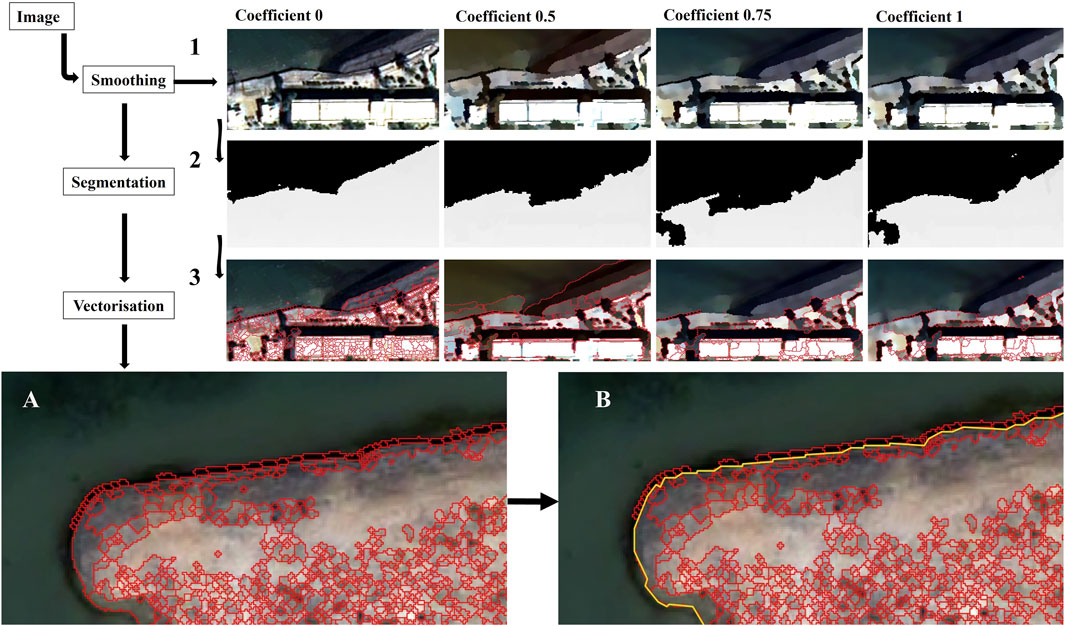
Figure 4. Coastline extraction process using image smoothing and segmentation (A). vectorized the segmented output (B). Extracted line corresponding to the chosen reference.

3.2.3 Automatic coastline recognition by image transformation

The methodology for automated coastline identification and extraction, as employed in this study, builds upon the approach developed by Gadal et al. (2023a). This technique relies on image transformation processes, specifically the application of the Minimum Noise Fraction (MNF) algorithm, followed by the detection of landscape structures through the use of a Laplacian filter applied to the MNF-transformed images.

• The MNF transformation serves to enhance image quality by isolating noise, thereby optimizing the data for subsequent analysis while reducing computational demands (Gadal et al., 2023a). Based on the spectral information of the bands and the variation in surface reflectivity, the images are decomposed and then reconstructed in the form of components with groups of pixels (Figure 5B).

• After analysing the MNF results, we improved the discrimination between geographical objects on the chosen MNF component using a 7 × 7 convolution Laplacian filter. The Laplacian filter highlights landscape structures based on areas of high change intensity (Gadal et al., 2023a), with good recognition of linear objects. For this case study, the newly produced MNF-2 (MNF on second spectral bande of the image) image was chosen for further processing, as it clearly identifies the different references for the position of the coastline. The application of the MNF and then the 7 × 7 Laplacian filter improves local discrimination between the geographical objects that characterise the study area (water, cliff edges, dry sand, wet sand, urban developments, etc.) by spatially contextualising them on surfaces measuring 3.5 m by 3.5 m (Figure 5).

Figure 5

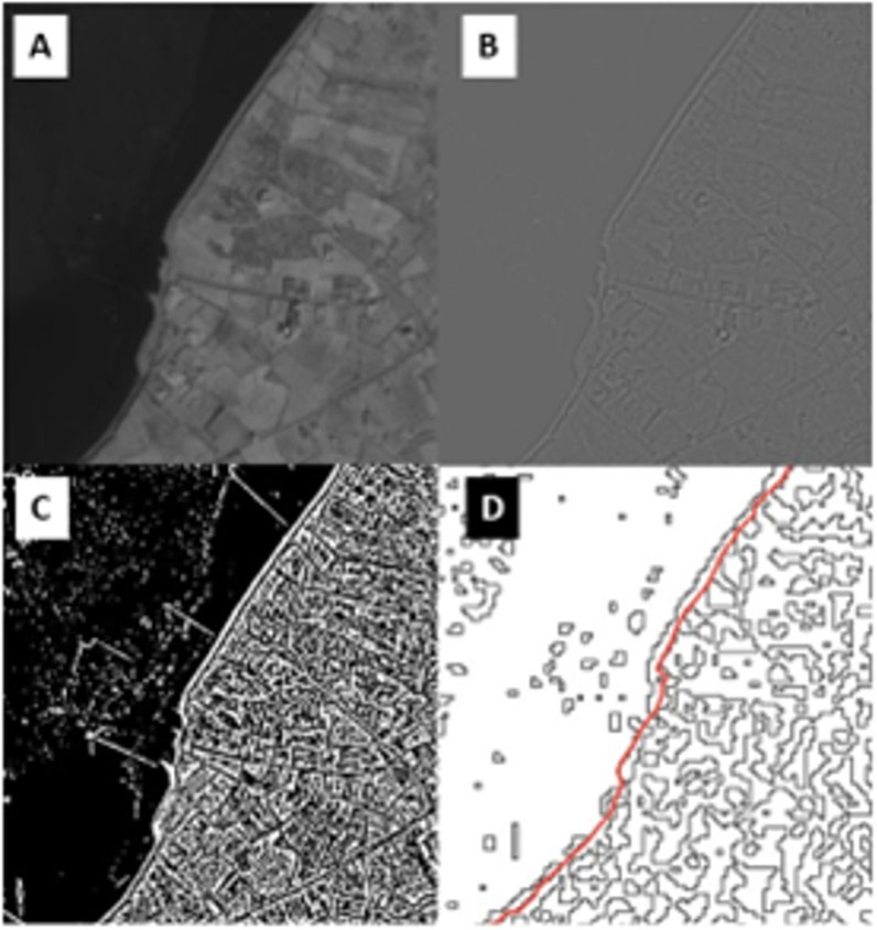
Figure 5. Different stages in the automatic extraction of the coastline (A) FMB transformation component which highlights the boundary between the different objects, (B) Laplacian filter with 7 × 7 pixel applied to the FMB component, (C) Selection from the raster calculator on the result of the Laplacian filter, (D) Vector conversion of the output after selection then simplified line conversion to obtain the coastline.

3.2.4 Extraction of coastlines using GIS

The results of the previous processing operations (image transformation and segmentation) are imported into the geographic information system, QGIS. For the results of the image transformation, we performed a thresholding in order to extract the coastline lines identified by the 7 × 7 Laplacian filter which selects values above two in order to ensure good harmony and continuity of the lines. The output is then converted into vector polygons and simplified lines, applying a simplification tolerance value equal to the image sampling (0.5 m). This eliminates the effects of pixelation (line with steps) and produces a line that we define as the reference coastline for each type of coastline in the study area (red line in Figure 5D).

Once the coastlines had been obtained, we imported them into a second GIS software package, ArcGIS, in order to calculate the kinematics of the coastline using the Digital Shoreline Analysis System (DSAS) module. To ensure that the results obtained can be properly interpreted, the overall margin of error (Table 1) needs to be calculated. This is determined using the following formulae (Gadal et al., 2023b; Thior et al., 2021):

$Ea=\sqrt{Egeore{f}^2+Eavdis{t}^2}$

and

$E_{\alpha }=\sqrt{EA{1}^2+EA{2}^2}/Period\left(t\right)$

Table 1

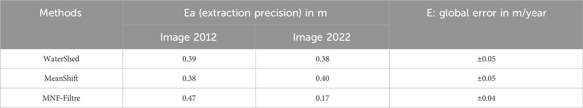
Table 1. Error margins.

Ea: margin of extraction error (in metres) for each year (2012 and 2022). Egeoref: margin of error linked to the georeferencing of images, which is obtained after orthorectification of each image and then georeferencing in relation to the reference data in question (Google satellite). As orthorectification was carried out on the OTB, georeferencing was carried out on ArcGIS using the adjustment transformation algorithm. This algorithm optimizes local accuracy and is based on the combination of a polynomial transformation and irregular triangulated network (TIN) interpolation techniques.² The adjustment transformation performs a polynomial transformation using two sets of control points and adjusts the control points locally to better match the target control points, using a TIN interpolation technique. Nine control points were taken into account for this study over a portion of the image approximately 4 km long and less than 2 km wide. ArcGIS provides a direct georeferencing error margin of 0.15 m for the 2012 image and 0.13 m for the 2022 image. Eavdist: margin of error linked to the accuracy of the extraction obtained using the average distances between the digitized coastlines and the automatically extracted coastlines. Eα: the overall margin of error in m/year.

3.3 Comparative statistics of coastline extraction methods using DSAS

In order to assess the performance of the different methods applied, we based ourselves on the statistical analysis of kinematics using the DSAS module in ArcGIS. The Digital Shoreline Analysis System (DSAS) is a statistical tool used to quantitatively measure geographical changes between several linear objects. Three indices were taken into account to assess the performance of the extraction methods.

1) The Net Shoreline Movement (NSM), which gives the net evolution statistics between two lines (in this case, it is the manually digitized coastline reference and the automatically extracted coastlines), 2) The Shoreline Change Envelope (SCE), which calculates the average distance between different coastlines. 3) The End Point Rate (EPR) calculates the net change and divides the values obtained by the difference between the most recent year of measurement (2022) and the oldest year (2012) to obtain the average annual rate of change.

4 Results

4.1 Validation of extracted coastlines

The results of the SCE index were used to assess the performance of each automatic extraction method in relation to the Digitized reference line. Table 2 shows the averages and standard deviations derived from the statistics for this index for the various methods. It can be seen that for all the automatic extraction methods the average distance is less than 1 m from the Digitized coastline. For the 2012 image, the variation in distances is smallest with the WaterShed algorithm, recording an average of 0.29 m, compared with 0.50 m for the MeanShift algorithm and 0.58 m for the combination of the MNF and Laplacian filter algorithms. For the 2022 image, we can see that the variation in distances is smaller with the WaterShed algorithm and the MNF-Laplacian filter combination, with 0.35 m and 0.39 m, respectively. The MeanShift algorithm recorded an average distance of 0.59 m. These average distances range from 0.29 m to 0.59 m, a maximum of 0.09 m compared with the spatial resolution of the Pléiades images. This accuracy performance with the different methods used can be explained by the quality of the Pléiades images, with a spatial resolution of 0.5 m and a spectral resolution ranging from visible to infrared and panchromatic, enabling a good characterisation and detection of geographical objects.

Table 2

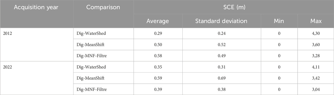
Table 2. Statistics showing the distance between the Digitized coastline and other extraction methods.

The variations between the features extracted by image transformation (MNF-Laplacian filter) and those Digitized can be explained by the choice of components for the minimum noise fraction used for further processing. The quality of the component depends on the spectral information in the base image and the quality of the pre-processing carried out. In addition, the orientation of the filter can have an impact on the accuracy of the result (Gadal et al., 2023b). In the case of MeanShift image segmentation, improving the sharpness of cluster edges can influence the output result. This improvement favors over-segmentation and therefore the detection of notches caused by differential erosion in the cliff zone. Indeed, it is on this cliff sector characterised by the presence of notches that the greatest fluctuations in the position of the coastline are noted. The differences between the features extracted by segmentation (WaterShed and MeanShift) on the two images (2012 and 2022) can be explained by the complexity of the reflectivity of the objects for each year as well as the land cover and also by the characteristics of the space, in particular the change in land occupation and therefore the difference in spectral information, given that the objects do not reflect in the same way (Figure 6). In addition, the segmentation algorithms used interpret the information differently, which may justify the variation in the position of the shoreline. This difference in interpretation is confirmed by the maximum distance between the extracted features and the Digitized one.

Figure 6

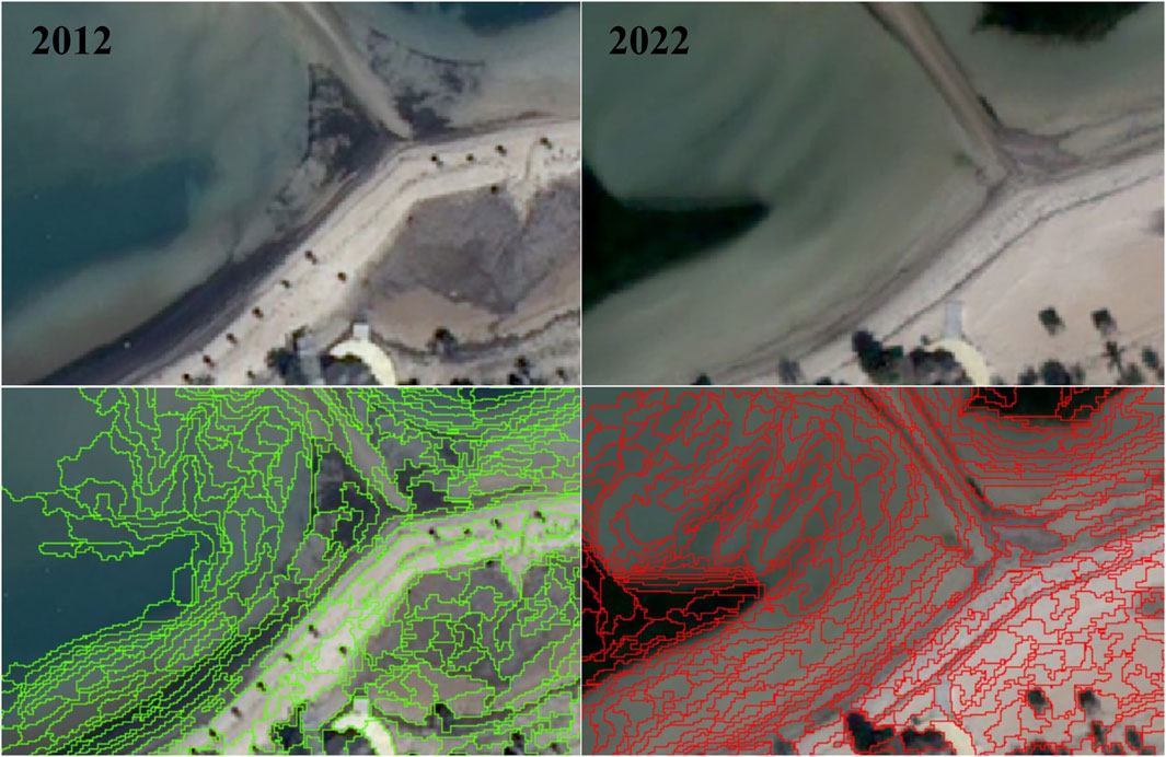
Figure 6. Characterisation of objects according to the characteristics of the zone and the method used for segmentation (MeanShift in this case).

4.2 Assessment of coastal evolution

In this section, we analyse the evolution of the coastline between 2012 and 2022 according to the different extraction methods. The analysis is based on the EPR and NSM indices. Table 3 shows the diachronic statistics for shoreline change using the different methods. The extraction methods using the WaterShed and MNF-Laplacian filter yield average change rates that closely align with those obtained through manual digitization, with values of -0.32 m/year for WaterShed, -0.29 m/year for the MNF-Laplacian filter, and -0.31 m/year for digitization. The coastlines extracted using the MeanShift algorithm show a more significant change, with an average of −0.33 m/year. Nevertheless, these results demonstrate that the three computational methods are very close in analysing changes in the coastline (difference of 0.03 m between the lowest and highest average).

Table 3

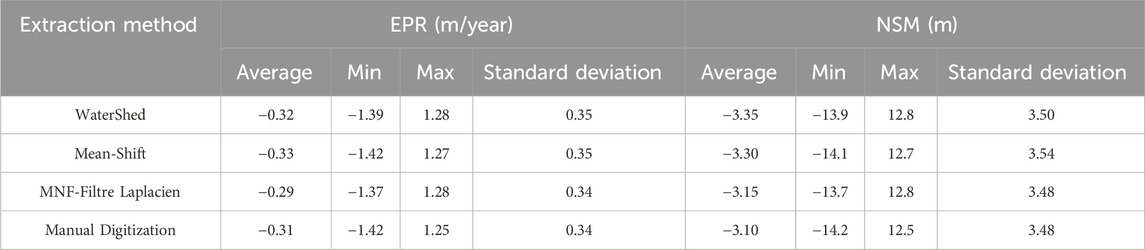
Table 3. Statistics (EPR and NSM) for shoreline change between 2012 and 2022, using each extraction method.

This performance is confirmed by the net change statistics for the NSM (Net Shoreline Movement) index, which shows a more or less uniform trend for the different methods. The greatest changes are seen in the sectors defined by significant mobility of the coastline. These include the cliff sector, marked by the presence of indentations, and the tourist sector around the Grand Hôtel. The Grand Hôtel sector is distinguished by the retreat of its tombolo (reaching −14 m) and a progradation of its southern part due to the development of this sector. Figure 7 shows the shoreline evolution curves between 2012 and 2022 based on the NSM index statistics for the different coastline extraction methods. The same variations in the shoreline can be seen over the entire profile studied, with different intensities depending on the method used. This justifies the performance of the different methods for automatic coastline extraction from Pléiades images.

Figure 7

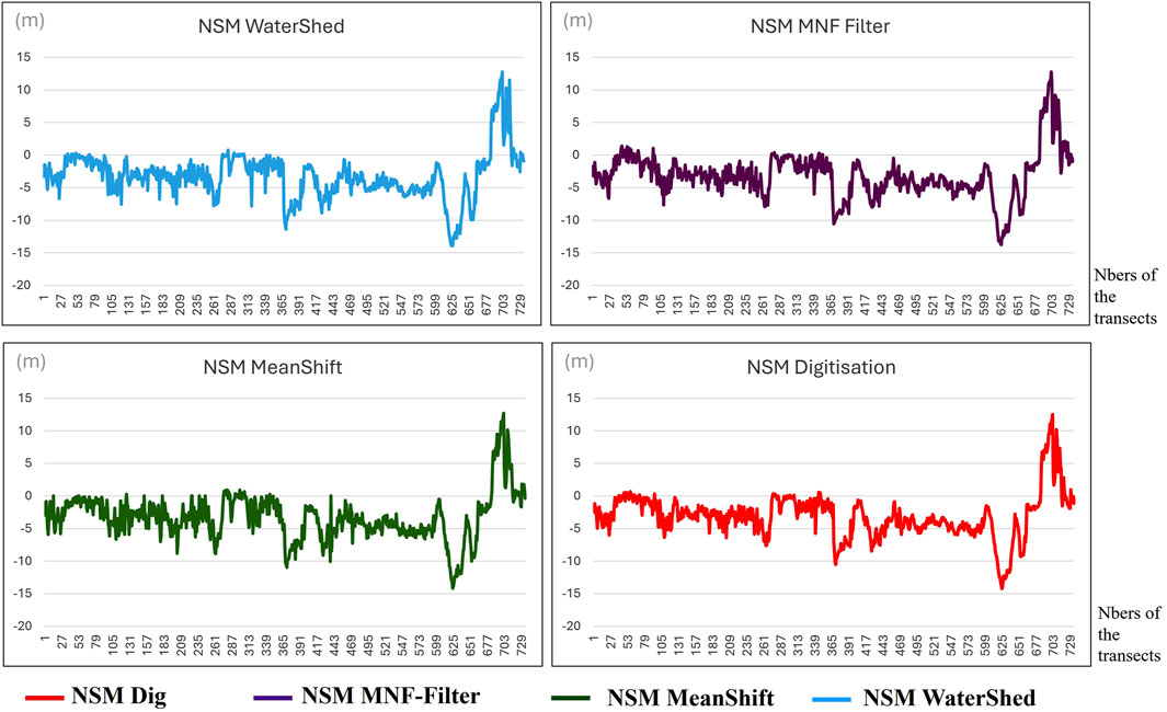
Figure 7. Comparison of NSM statistics for the different extraction methods used.

As the study area features different types of coastline (cliff coast, sandy coast and developed coast), it is interesting to determine the performance of each method on the different types of coastline.

4.3 Performance of extraction methods in relation to coast types

As mentioned above, the coastline of the study area features different coastlines. Over a stretch of coastline of around 4 km, the coast is defined by a combination of cliffs/micro-cliffs (between 1.5 m and around 4 m high), a low, sandy stretch of coast (very limited in extent), and a built-up coastal stretch. Depending on the characteristics of each type of coastline, the reflectivity of objects and spectral information, the coastline is interpreted differently. As a result, the accuracy of coastline detection will differ from one coastal sector to another depending on the extraction method applied. Figure 8 shows the results of the classification of features in the form of polygons by each extraction method, on each type of coastline within the study area. This comparison of the different results shows that extraction using the WaterShed algorithm performs better on urbanised coastlines and on sandy coasts. This algorithm clearly detects the shoreline in the developed sectors, as well as in the zones marked by the presence of wet or non-wet sand, indicators of the limit of humectation. On the other hand, the detection of the cliff coastline is more complex. This complexity is explained by the shadows on the cliffs visible in the images, which affect the accuracy of coastline detection. For the other two automatic extraction methods (MNF-Laplacian filter and MeanShift), coastline detection is more challenging on the different types of coastline. Unlike the WaterShed algorithm, which clearly identifies the boundary between the water and the reference lines, these two algorithms over-segment the image and in addition to these lines highlight other boundary features between objects on the different types of coastline. This can be explained by the good distinction of objects favoured by the spatial and spectral characteristics of the Pléiades images used for this study. In addition, due to the study area’s low bathymetry, shoal areas are well identifiable and their boundaries are well represented. In addition, these two methods (MNF-Laplacian filter and MeanShift) transform the images after smoothing for segmentation, justifying the fact that the images are reclassified according to the spectral information and the quality of the smoothed image used for segmentation. Nevertheless, by superimposing the results of these extraction methods on the satellite image, it is possible to clearly identify the corresponding reference line for each type of coastline. Extraction using the MeanShift method, which highlights more details, in particular the cliff notches, therefore performs best on cliff coasts (Figure 8).

Figure 8

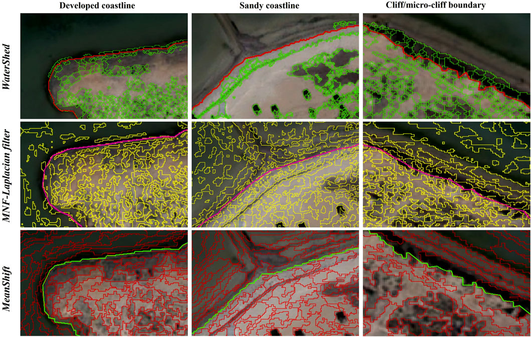
Figure 8. Performance of the different extraction methods applied (WaterShed, MNF-Laplacien filter, MeanShift) in the relation to the types of coastlines that characterise the study area (developed coastline, sandy coastline and cliff boundary). The WaterShed algorithm detects the shoreline more easily.

If we consider the percentage (Table 4) of coastline extracted by each method, we can see that the method based on the combination of the MNF and the Laplacian filter performs better, having extracted 98.8% of the coastline studied, compared with 98.5% for the MeanShift and 97.4% for the Watershed. The low percentage of coastline extracted by the WaterShed can be explained by the algorithm’s segmentation method, which results in the discontinuity of the shoreline in certain sectors where the areas of the pixel classes are larger. In addition, the shadows generated by the geographical objects that define the study area (trees, cliffs) interfere with the detection of the shoreline and hence the discontinuity of the coastline (Figure 9).

Table 4

Table 4. Statistics from the EPR index showing the performance of the different extraction methods.

Figure 9

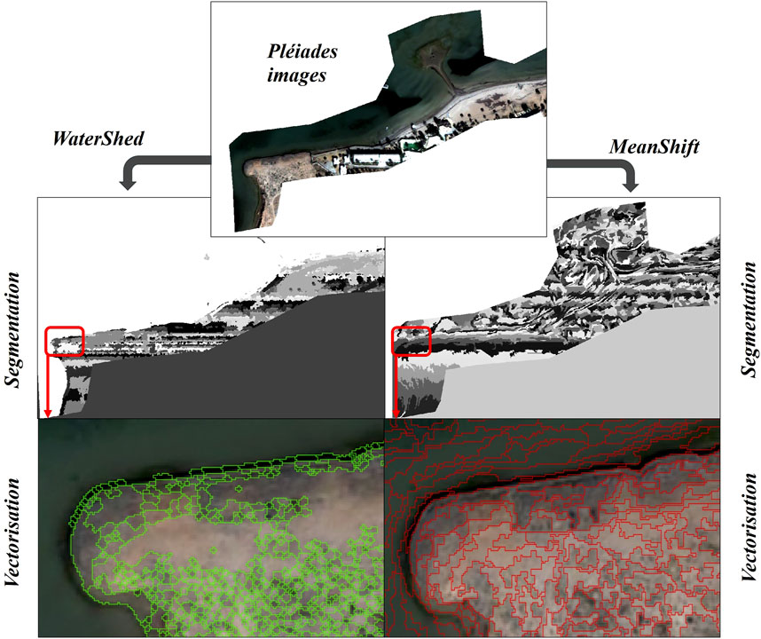
Figure 9. Image segmentation using the WaterShed and MeanShift algorithms.

4.4 Evolution of the shoreline between 2012 and 2022: an overall retreat of the shoreline over 10 years

After analysing the performance of the different shoreline extraction methods used (WaterShed, MeanShift and MNF-Laplacian filter) on each type of coastline, we extracted the shoreline for each sector according to the best performing method. For urbanised and sandy coasts, the features extracted by WaterShed were used. For cliff coasts, on the other hand, the features extracted by MeanShift were taken into account. The coastlines obtained were used to quantify recent changes in the shoreline over a 10-year period from 2012 to 2022, from Karaba beach to the Sidi Frej tourist area, including the Borj El H’ssar archaeological site. The results of kinematics based on the EPR index were used for this analysis of the diachronic evolution of the coastline. The statistics show an overall retreat of the shoreline with an average of −0.33 m/year (margin of error ±0.05 m/year). On a geomorphological level, this recession is caused by the continuous action of hydrodynamic agents (waves, currents) eroding the shoreline. There is also the difference in rock types, which encourages differential erosion and, as a result, the collapse of boulders precisely in the cliff areas. In addition the absence of sedimentary input from inland towards the shore, combined with the rise in sea level (IPCC, 2022) and the subsidence that has occurred in the area since ancient times (Oueslati, 1995b), means that the shoreline is continually retreating. The sedimentary input in this sector comes mainly from the erosion of the cliffs, whose blocks are left scattered along the foreshore. These blocks gradually disintegrate on contact with the water and the sediment is transported towards the south of archipelago following the prevailing longshore drift. As a result, the shoreline is retreating across the entire study area. This erosion is greatest at Grand Hôtel beach and Borj El H’ssar, with rates of −0.83 m/year and −0.34 m/year respectively. The erosion of the Grand Hôtel beach is attributable to the presence of loose sand, easily erodible. It has been reflected in the nibbling away of the tombolo in front of the hotel, which favoured the accumulation of sediment transported by the longshore drift. This tombolo also enabled the Grand Hôtel beach to benefit from the contributions of the sediment coming from the erosion of the Borj El H’ssar cliffs (Oueslati, 2004; Etienne and Etienne, 2014). However, this arrangement no longer entirely plays its role, as shown by the statistics for trends between 2012 and 2022, which are contrary to those of Etienne, (2014) showing progradation of the shoreline in this same sector between 1960 and 2010. The ineffectiveness of this tombolo can be explained by the fragility of the sediments that characterise the beach, but also by the intensification of hydrodynamic agents. On the other hand, to the south of the Grand Hôtel, there has been significant progradation. This accretion, with an average of +0.66 m/year, is due to the installation of a structure designed to protect the tourist facilities in this sector. In the Borj El H’ssar area, coastal erosion is evident, with an average of −0.34 m/year. This sector, which supplies sediment (Oueslati, 2004; Etienne, 2014) in the form of debris torn from the cliffs, has long been exposed to coastal erosion (Oueslati,1995a, Oueslati,1995b; Oueslati, 2004). The archaeological remains that have come to light over the years, most of which are underwater at high tide or form the point where the waves lap (in the foreground of the cliffs), confirm this retreat of the shoreline. Faced with this situation of continuous retreat of the shoreline, local people are implementing adaptation strategies by building protective walls in front of their properties. One of these protective walls, built before 2012 along a private individual’s premises and constituting the point of wave erosion, is the reason for the stability of the coastline between the Borj El H’ssar site and the cliff zone (Figure 10). In fact, the presence of these facilities ensures a stability that can be characterized as relative and ‘temporary’ and may raise the debate about the effectiveness of these infrastructures and their participation in the intensification of erosive action (Oueslati, 2010). Observation of the current morphology of the coast reveals its convex-concave appearance, proof of the difference in intensity of the action of the dynamic agents, which are more apparent in the southern part of the protective wall.

Figure 10

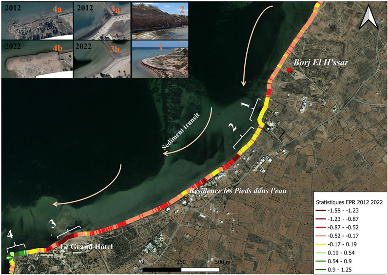
Figure 10. Summary of the evolution of the coastline between 2012 and 2022 based on the End Point Rate, showing areas of erosion (red: negative values), areas of progradation (green: positive values) and areas of stability (yellow).

5 Conclusion

This study assessed the performance of various methods for extracting complex coastlines from very high-resolution Pléiades images. One of the methods used is based on image transformation using a combination of MNF and Laplacian filter algorithms. The other extraction method is based on image segmentation using the WaterShed and MeanShift algorithms. It was also essential to assess the performance of these extraction methods on the types of coastlines that define the study area. The accuracy of the automatic coastline extraction of the different methods was assessed by comparing their average distances from the Digitized coastline. Statistics for the Shoreline Change Envelope, Net Shoreline Movement and End Point Rate indices were taken into account, making it possible to quantify fluctuations in the reference line detected by each method, as well as diachronic changes in the shoreline over the 10-year period considered (2012–2022). Analysis of the results shows that the extraction method based on the WaterShed algorithm performs best in terms of accuracy in relation to the coastlines obtained by Digitization, recording the lowest average distances for the two images considered: 0.29 m for the 2012 image and 0.35 m for the 2022 image, compared with 0.58 m in 2012 and 0.39 m in 2022 for the MNF-Laplacian filter method and 0.50 m in 2012 and 0.59 m in 2022 for the MeanShift method.

In terms of the percentage of coastline extracted, the method based on the MNF-Laplacian filter combination performs best, with 98.8% of coastline extracted. It is followed by the MeanShift method with 98.5% of coastline extracted. The WaterShed method had the lowest percentage, with 97.4% of ribs extracted. As for the performance of the extraction methods by type of coastline, the results show that the WaterShed method performs best. It detects the shoreline perfectly on developed coasts and on sandy coasts. On cliff coasts, on the other hand, the MeanShift and MNF-Laplacian filter algorithms perform better. However, detecting the coastline on these cliff areas is complex due to the shadow cast by the cliffs when the satellite images are taken and the over-segmentation of the images.

By taking into account the coastline extracted using the most effective method for each type of coastline (WaterShed for developed and sandy coastlines, MeanShift for cliff coasts), we have been able to determine how the shoreline has changed over 10 years (2012–2022). This shows an overall retreat of the shoreline, with an average of −0.33 m/year. This erosion is more critical at the Grand Hôtel beach (−0.88 m/year) and around the Borj El H’ssar archaeological site it is near the average value (−0.34 m/year). This erosion leads to the destruction of archaeological remains on the cliffs and amplifies the vulnerability of human settlements, highlighting the critical need for reliable methods to monitor shoreline dynamics and support the management of these coastal areas. However, the use of only two images is a limitation in terms of the reliability of the dynamics characterising the study area. This is due to the lack of Pléiades archive images (only one in 2012). For this reason, we were obliged to carry out the study using the 2012 archive image and the image acquired by tasking in 2022. Nevertheless, these methods could be applied to other study areas in order to verify their transposability and performance.

Data availability statement

The datasets presented in this article are not readily available because Images processed are not shareable. Requests to access the datasets should be directed to bHVjLmRpYXR0YUBjZXJlZ2UuZnI=.

Author contributions

LD: Data curation, Data acquisition, Formal Analysis, Investigation, Methodology, Software, Writing – original draft. KS: Data acquisition, investigation, Writing original draft, Writing – review and editing. ZA: Writing original draft, investigation. SB: Writing original draft, investigation. AD: Writing original draft, investigation. AO: Writing original draft, Writing - review and editing, investigation. LL: Data acquisition, Methodology, Software, Writing original draft.

Funding

The author(s) declare that financial support was received for the research and/or publication of this article. Part of this work (site visit and ground-truthing) received support from the French government under the France 2030 investment plan, as part of the Initiative d’Excellence d’Aix-Marseille Université - A*MIDEX - Institute for Mediterranean Archaeology ARKAIA (AMX-19-IET-003).

Acknowledgments

We are grateful to the 2022 Tunisian-French mission working on the salt heritage in Kerkena Project (direction AD, INP and KS, CNRS, with funding from the Fyssen Foundation), for allowing us to use their geo-referenced survey points. We also wish to thank our reviewers for their helpful suggestions.

Conflict of interest

The authors declare that the research was conducted in the absence of any commercial or financial relationships that could be construed as a potential conflict of interest.

Generative AI statement

The author(s) declare that no Generative AI was used in the creation of this manuscript.

Publisher’s note

All claims expressed in this article are solely those of the authors and do not necessarily represent those of their affiliated organizations, or those of the publisher, the editors and the reviewers. Any product that may be evaluated in this article, or claim that may be made by its manufacturer, is not guaranteed or endorsed by the publisher.

Footnotes

¹DINAMIS (https://dinamis.data-terra.org/catalogue/)

²As highlighted by ESRI.

References

Amar, R. (2010). Impact de l'anthropisation sur la biodiversité et le fonctionnement des écosystèmes marins. Exemple de la Manche-mer du nord. Vertigo la revue électronique en sciences de l'environnement, hors-série 8, doi:10.4000/vertigo.10129

CrossRef Full Text | Google Scholar

Anthony, E. J. (2008). Shore processes and their paleoenvironmental applications. Amsterdam: Elsevier.

Google Scholar

Beck, G., Azzag, H., Lebbah, M., Duong, T., and Cérin, C. (2018). Mean-shift: Clustering scalable et distribué. EGC, 415–425. Available online at: https://www.mvstat.net/tduong/research/publications/beck-et-al-2018-egc.pdf.

Google Scholar

Bengoufa, S., Niculescu, S., Mihoubi, M. K., Belkessa, R., Rami, A., Rabehi, W., et al. (2021). Etude comparative des méthodes de classification pixel par pixel et orientée objet pour la détection et l’extraction automatique du trait de côte (cas du secteur côtier de Mostagan à l’Ouest algérien). Contribution du spatial aux enjeux de l’eau, Marseille, 8-10 juin 2020, France, in Unpublished conference paper. Available online at: https://www.researchgate.net/publication/351783302.

Google Scholar

Ben Mustapha, K. (2007). Démosponges littorales des îles de Kerkennah (Tunisie). Bull. de l’Institut Natl. des Sci. Technol. de Mer 34, 37–59. Available online at: http://hdl.handle.net/1834/4208.

Google Scholar

Beucher, S. (1992). The Watershed transformation applied to image segmentation. Scanning Microsc. 6. Available online at: https://digitalcommons.usu.edu/microscopy/vol1992/iss6/28.

Google Scholar

Boussetta, A., Niculescu, S., Bengoufa, S., and Zagrarni, M. F. (2023). Deep and machine learning methods for the (semi-)automatic extraction of sandy shoreline and erosion risk assessment basing on remote sensing data (case of Jerba island, Tunisia). Remote Sens. Appl. Soc. Environ. 32, 101084. doi:10.1016/j.rsase.2023.101084

CrossRef Full Text | Google Scholar

Diatta, L. S., Fall, L. C. A., and Sané, Y. (2022). Impacts de la dynamique du littoral entre Cabrousse et Boudiédiète (commune de Diembéring), Basse-Casamance. Rev. Esp. Société Marocaine, 58. doi:10.34874/IMIST.PRSM/EGSM/31136

CrossRef Full Text | Google Scholar

Etienne, L. (2014). Accentuation récente de la vulnérabilité liée à la mobilité du trait de côte et à la salinisation des sols dans l’Archipel de Kerkennah (Tunisie). Sorbonne Paris Cité; Sfax University Faculté des Lettres et Sciences Humaines. Available online at: https://theses.hal.science/tel-01075029/file/LETIENNE-Manuscrit-These.pdf.

Google Scholar

Gadal, S., and Gloaguen, T. (2023a). The evolution of the south-eastern sea coastline between 1988 and 2018 by remote sensing, in GISTAM 2023 9^th international conference on geographical information systems theory, applications and management, ATHENA, 37–47. Available online at: https://hal.science/hal-04080526v2.

Google Scholar

Gadal, S., and Gloaguen, T. (2023b). Performance of landsat 8 OLI and sentinel 2 MSI images based on MNF versus PCA algorithms and convolution operators for automatic Lithuanian coastline extraction. SN Comput. Sci. 5. doi:10.1007/s42979-024-02623-9

CrossRef Full Text | Google Scholar

Gustave, M. (2022). L’action publique locale à l’épreuve de l’Anthropocène: une étude comparative entre deux territoires littoraux atlantiques. Ph.D Thesis. La Rochelle University. Available online at: https://theses.hal.science/tel-04190085/file/2022GUSTAVE197441.pdf.

Google Scholar

Hugueny, P. A. (2014). Développement d’un outil de segmentation et de classification semi-automatique de pierres. Mémoire, Sci. l’ingénieur, Dumas. Available online at: https://dumas.ccsd.cnrs.fr/dumas-01168266/file/HUGUENY%20Pierre-Alban.pdf.

Google Scholar

IPPC (2022). Climate Change 2022: Mitigation of Climate Change. Available online at: https://www.ipcc.ch/report/ar6/wg3/.

Google Scholar

Juigner, M., Robin, M., Fattal, P., Maanan, M., Le Guern, C., Gouguet, L., et al. (2012). Cinématique d’un trait de côte sableux en Vendée entre 1920 et 2010. Méthode et analyse. Dynamiques Environnementales. J. Internation. Géosci. Environm. 29–39. Available online at: https://www.researchgate.net/publication/278624019.

Google Scholar

Lefèvre, S. (2009). Segmentation par ligne de partage des eaux avec Marqueurs spatiaux et spectraux, in Conférence GRETSI sur le Traitement du Signal et des Images. Dijon, France. Available online at: https://www.gretsi.fr/data/colloque/pdf/2009_001-0426_29101.pdf.

Google Scholar

Louati, M., Saïdi, H., and Zargouni, F. (2014). Shoreline change assessment using remote sensing and GIS techniques: a case study of the Medjerda delta coast, Tunisia. Arabian J. Geosciences 8, 4239–4255. doi:10.1007/s12517-014-1472-1

CrossRef Full Text | Google Scholar

Mallet, C., Michot, A., De la Torre, Y., Lafon, V., Robin, M., and Provoteaux, B. (2012). Synthèse de référence des techniques de suivi du trait de côte. Rapp. final BRGM/rp- 60616-FR. Available online at: https://infoterre.brgm.fr/rapports/RP-60616-FR.pdf.

Google Scholar

Maur-Férec, C., and Morel, V. (2004). L’érosion sur la frange côtière: un exemple de gestion des risques. Natures Sci. Sociétés 12, 263–273. Available online at: https://www.cairn.info/revue-natures-sciences-societes-2004-3-page-263.htm.

Google Scholar

Niang-Diop, I. (1995). L’érosion côtière sur la petite côte du Sénégal à partir de l’exemple de Rufisque passé-présent-futur. PhD Thesis. Paris: Angers University, Orstom. Available online at: https://horizon.documentation.ird.fr/exl-doc/pleins_textes/pleins_textes_6/TDM/010008221.pdf.

Google Scholar

Oueslati, A. (1995a). The evolution of low Tunisian coasts in historical times: from progradation to erosion and salinization. Quat. Int. 29-30, 41–47. doi:10.1016/1040-6182(95)00006-5

CrossRef Full Text | Google Scholar

Oueslati, A. (1995b). Les îles de la Tunisie: paysages et milieux naturels: genèse, évolution et aptitude à l'aménagement d'après les repères de la géomorphologie, de l'archéologie et de l'occupation humaine récente. Tunis.

Google Scholar

Oueslati, A. (2004). Littoral et aménagement en Tunisie. Tunis: Publications de la Faculté des Sciences Humaines et Sociales.

Google Scholar

Oueslati, A. (2010). Plages et urbanisation en Tunisie: des avatars de l’expérience du XX^e siècle aux incertitudes de l’avenir. Rev. Méditerranée 115, 103–116. doi:10.4000/mediterranee.4928

CrossRef Full Text | Google Scholar

Paskoff, R. (2004). L’érosion des côtes: le cas des plages de l’île de Jerba (Tunisie). Hydrosci. houille blache 90, 48–51. doi:10.1051/lhb:200401006

CrossRef Full Text | Google Scholar

Thior, M., Sy, A. A., Cisse, I., Dieye, E. B., Sane, T., Ba, B. D., et al. (2021). Approche cartographique de l'évolution du trait de côte dans l'estuaire de la Casamance. Mappemonde 131. doi:10.4000/mappemonde.5939

CrossRef Full Text | Google Scholar

Zegaoua, F. (2012). Segmentation adaptative des images mono-spectrales par coopération de méthodes. Master Thesis. Saad Dahlab de Blida University. Available online at: http://di.univ-blida.dz:8080/jspui/handle/123456789/12684.

Google Scholar