Elastic and inelastic LiDAR pulse return phenomenology in coastal underwater biological substrates

In the context of current and future climate-related environmental changes, the development of innovative underwater substrate detection, classification and imaging methods at large spatial scales is key in monitoring and understanding changes from stresses occurring in coastal ocean areas. This development will help understand the spatial distribution and abundance patterns of marine primary producers and ecosystem service providers such as macroalgae, eelgrass and other important ecosystem components such as coral, and can provide insights into future ecosystem response and better management practices. The objective of the current work is to describe an analysis of data acquired by full waveform underwater fluorescence LiDAR, designed for detecting, imaging, and generating 3D point clouds of inert and biological substrates capable of fluorescence. Since the instrument is designed as a small form-factor AUV payload operating at standoff distances of 5–10 m, we chose to implement full-waveform (2.5 Gs/s), pulsed 532 nm laser, capable of generating 1 ns pulses of up to 2.5 uJ at a 200 kHz repetition rate to generate elastic (532 nm) and inelastic (685 nm) 3D point clouds for underwater benthic mapping. Analysis of these acquired waveforms has shown opportunities for improving the point cloud density, by identifying multiple returns within the same waveform, when present. Pulse return processing methods such as Gaussian decomposition and Richardson-Lucy deconvolution are evaluated on data acquired during LiDAR sea-trials over various bottom substrates. As the present LiDAR beam footprint is relatively small to maximize energy density for longer range detection and potential fluorescence response, the number of detected returns per pulse ranges from one in the case of a bare benthic substrate and up to 2 or 3, in areas where for example, macroalgae, kelp, corals and/or other substrates characterized by a vertical structure are present.

1 Introduction

Remote sensing has been instrumental from its beginnings in providing means to study diverse environments at large spatial scales, various spatial resolution and in a timely manner (e.g., Landsat 1 (1972) to Landsat 9 ongoing program, NASA, 2023). Beyond the classic “passive” (i.e., no artificial light source) remote sensing methods initially developed, pulsed laser technology, from which lidar (Light Detection and Ranging) methodology has been developed, has additionally provided means to interrogate remote surfaces and environments by specifically incorporating laser pulse Time-of-Flight (ToF) measurement in remote detection of spectral signature. Allowing a 3-dimensional or x, y and z (time, or range) measurement within an environment, ToF measurement feature can be used to recreate a 3D point cloud or map of the studied environment. To date, these methods have most often been used in above-ground or above-water situations. However, bathymetric lidar applications are becoming increasingly common (see for example, IceSat2 Gleason et al. (2021)), as are ocean water column profiling applications (Jamet et al., 2019; Zhou et al., 2022). This difference in the number of developed applications can be in part explained by the difficulty in operating underwater. However, recent underwater AUV-based (Autonomous Underwater Vehicle) technological advances (e.g., Kongsberg Hugin/Remus models, other small AUV providers) are giving the means to facilitate underwater remote sensing surveys. These new opportunities for more rapid assessment of underwater environments are and will be increasingly important in monitoring important ecosystems through environmental changes and human associated impacts.

In providing new solutions to monitor and better understand ongoing changes in the underwater and marine environment, the current work is to describe an analysis of data acquired by newly developed, full waveform underwater fluorescence lidar, which we designed for detecting, imaging, and generating 3D point clouds of inert and biological substrates capable of fluorescence. The lidar was initially tested in the form of a ship-side pole-mounted small research vessel instrument, with the objective of future integration onto REMUS 100 type AUVs or similar-sized units capable of additional scientific instrument payloads. Operating via the principle of rapidly emitting laser pulses (i.e., 532 nm wavelength) at high frequency and digitizing subsequent reflections, or « returns », via highly sensitive optical sensors, a 3D visualization of the underlying environment can be recreated. In its current multispectral configuration, laser pulse returns are recorded as either from reflected or backscattered at 532 nm from a particle or surface, or from fluorescence emitted from water column constituents such as chlorophyll containing microalgae, from a macroalgal or coral surface. Whereas discrete return LiDARs are configured to record a specific number of returns (e.g., 4–5), our instrument is full waveform and currently capable of digitizing pulse returns at the high-speed rate of 2.5 Giga samples per second, per optical channel. Hence, the acquired data gives the possibility to analyze not only surfaces of interest, but also study the water column and its constituents from the full-waveform datasets.

Since fluorescence emitted by chl-a is rapidly absorbed in water (see Absorption by pure sea water (Mobley, 1994), detecting algal, plant or coral fluorescent substrates by their emission must be done within short to medium range (e.g., 2–10 m), relatively. Whereas fluorescence emission intensity may be variable and possibly enhanced by a stronger exciting laser pulse, elastic (i.e., 532 nm) returns are usually much stronger as they are actual reflections from a pulse and much less subject to absorption in water at this wavelength (Mobley, 1994). This « elastic » reflectance response at 532 nm technically has the furthest reach and is useful in retrieving bathymetry, but also potentially providing a good representation of structural 3D point-cloud. Fluorescence may also provide for 3D point cloud structure, but as emission is more Lambertian (i.e., towards all directions), observed intensity will be lower from the even distribution of light from the emitting surface, compounded with the effects of high light absorption in the far red.

Full-waveform lidar has the advantage of providing a detailed time-history of the light signal received immediately after the lidar’s laser pulse, from backscatter, or until it is attenuated by the imaging medium and/or pulse “returns” (or backscattering: elastic or inelastic) can no longer reach the optical receiver. While it is possible to easily extract information, for example, the intensity of only highest pulse return peak (often corresponding to a bottom substrate) in an underwater benthic imaging context, more detailed information can be extracted, using deconvolution and decomposition methods (see Zhou et al. (2017) for a detailed analysis and comparison). Deconvolution can help to remove imaging system noise (i.e., electronic) from the recorded signal waveform, as well as to better isolate overlapping pulse returns (i.e., close in range) as how they should be according to the outgoing laser pulse width and amplitude. Two methods have been retained for having demonstrated their applicability to a range of situations (e.g., large, and small footprint lidar), Richardson-Lucy (RL) (Fish et al., 1995; Nordin, 2006; Wu et al., 2011) and Gold’s algorithm (Hancock et al., 2017; Zhou et al. 2017). Further, decomposition of the waveform, into sub-component peaks, can provide information as to where these subsequent peak returns are, and their intensity. While there are other approaches possible, use of Gaussian model has shown to be sufficient in identifying waveform peak components in a variety of imaging conditions and for various instruments (e.g., Gwenzi and Lefsky, 2014; Hancock et al., 2017; Wu et al., 2011; Mountrakis and Li, 2017; Fieber et al., 2015). These methods are essential in generating more detailed 3D point clouds and better range resolution for the different surfaces or objects detected. However, they have mostly been applied to terrestrial habitat characterization (e.g., forest canopy structure). It is in this work that we investigate comparing lidar pulse return phenomenology, and subsequent signal waveform processing to optimize detection of additional peak returns and provide more detailed and accurate 3D point cloud data.

The aim of this study is to demonstrate the capabilities of full waveform underwater fluorescence lidar detection and imaging for coastal benthic surveys of key ecosystem components such as macroalgae/kelp, coral and other common associated inert substrates. Emphasis is put on describing individual lidar pulse returns in their phenomenology and between these substrates, including elastic reflectance, multiple forward scatter, tail-end backscatter of the water column and hard target returns at midwater and bottom. Further, pulse return processing and optimization methods are demonstrated using Richardson-Lucy (RL) and Gold’s algorithms for deconvolution to better identify and isolate additional peaks, and Gaussian decomposition for peak location (i.e., for Time-of-Flight measurement, intensity and width (while not used here)). These results are presented to provide the next steps in supporting the development and use of underwater lidar AUV surveys for detection and mapping of biological benthic substrates at larger spatial scales. By this work, underwater lidar imaging and fluorescence detection can be seen as an additional and precise tool for characterizing coastal benthic and biological substrate at larger spatial scales, by improving upon satellite and aerial surveys by reducing the spatial and spectral resolution lowering effects of the air-water interface and increased measurement distances.

2 Materials and methods

2.1 Lidar instrument characteristics

The underwater fluorescence lidar described and used in this study is composed of the usual lidar imaging components including optical transmitter and receiver assemblies, control, and data acquisition electronics, all contained within a 100 m depth-rated housing with acrylic viewport (see Figure 1 for simplified system and components schematic). The complete housing is currently made to fit as an optical payload section onto a REMUS 100 AUV but could be adapted to equal diameter or larger AUV payload formats. The current onboard laser emitter can provide a pulse energy which varies with Pulse Repetition Rate (PRR) (see main laser in Table 1). For the data presented in this work, a PRR of 200 kHz was selected to optimize point density on the sea bottom which is dependent on the imaging platform speed and distance to bottom. Laser line scanning was achieved by alignment of the laser onto a constant speed rotating multifaceted polygon via which the timing of laser pulse emissions is synchronized to the signal acquisition.

Figure 1

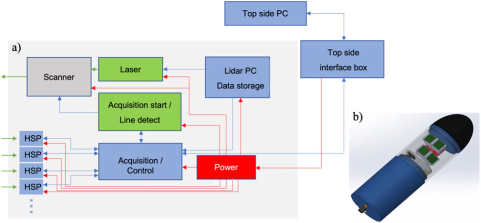
Figure 1. Schematic of (a) system components for the underwater fluorescence lidar and (b) assembled components showing, from left, electronics/power connector, anodized heatsink section, clear acrylic detector section, front removable hydrodynamic endcap. Four High Speed Photodetectors (HSP) (e.g., PMTs) with interchangeable filters allow signal acquisition for underwater elastic (i.e., 532 nm) and inelastic (e.g., 685 nm) 3D point cloud generation and benthic imaging when oriented towards and within imaging distance from the sea bottom.

Table 1

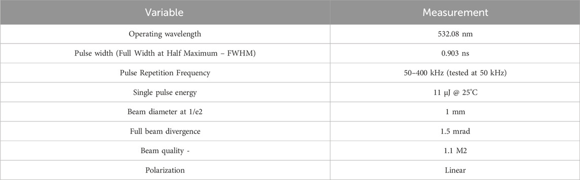
Table 1. Laser emitter characteristics.

2.2 Receiver assembly

Operating at a 2.5 Gsps rate per channel, the high-speed digitizer is built for acquiring two channels simultaneously (four channels in sequence of two simultaneous channels), providing a pulse sampling interval nearing 400 ps for a 160 ns duration. Using a high sampling rate oscilloscope operating at 40 ps per sample or 25 Gsps, the lidar’s system impulse response with PMTs (i.e., laser impulse response convolved with the PMT impulse response) was measured to be approximately 3.68 ns, while laser outgoing impulse response was measured to be 1.696 ns The unit is controlled via 10 m Gigabit Ethernet + power cable.

The receiver optics are divided into four independent optical channels where each has its own PMT. Each unit is time-gated to restrict light amplification during times between pulses where no signal is expected, based on the sampling frequency and pulse repetition rate. These can be configured in elastic (i.e., 532 nm narrowband filter) or inelastic (i.e., 685 nm narrowband filter, used in this study). The PMTs are arranged in pairs within a frame inside the acrylic housing (Figure 4b). Each pair can be rotated along its central attachment point within the frame to allow a variable overlap between the four detectors. A wider spread between individual PMTs and hence, slight overlap between PMT FOVs offers a 120-degree elastic FOV, suitable for wide swath elastic imaging (4 × 532 nm narrow bandpass filters required). A more important overlap provides both elastic and inelastic imaging of the same target scene, however with a smaller FOV (60-degree FOV, both elastic and inelastic). Each inelastic receiver had a FOV of 30-deg full angle. Both configurations were used in this study, where in the latter, the two forward PMTs are set for elastic, followed by and in-line with the inelastic PMTs closer to the central lidar body. A Fresnel lens is fitted over each PMT to collect as much light as possible and focus it over each sensor’s active surface area. Each low-profile lens is preceded by an individual and interchangeable narrowband filter corresponding to elastic (i.e., 532 nm) or inelastic (i.e., 685 nm) target signals.

To operate in underwater situations as part of an AUV optical payload, where obstacles may be present and need to be avoided (e.g., under ice ridges and keels, boulder fields), the lidar was designed to operate at standoff distances between 5–10 m. Water column turbidity being of major concern in coastal waters, inelastic photon signal attenuation is especially important in the red - 685 nm - region and restricting in terms of maximum imaging range. Hence, the design is currently limited to this range for fluorescence/inelastic imaging. The range can however be extended, up to 20+ meters in exceptionally clear water but the elastic response from the bottom substrate may be the only discernable signal, except fluorescence from phytoplankton and/or particle backscattering associated to the upper shallower water column or closer to the unit when deployed at greater depth in AUV mode. Lidar optical and electrical component selection was therefore a compromise between laser/electronics energy consumption, payload size suitable for a small AUV as well as expected fluorescence from target substrates (i.e., estimated quantum yield of fluorescence).

While operating at 10 m from the substrate and moving at a forward speed of 2 m/s (3.9 knots), image/point cloud resolution is approximately 5 cm (horizontal) by 5 cm (vertical). Considering this distance to target of 10 m and that field of view in elastic + inelastic configuration is approximately 60°, imaging swath width is estimated to 11.54 m (or for perspective, 5.8 m swath width at 5 m distance).

2.3 Lidar imaging geometry

The lidar instrument considered in this study can be characterized as a nearly monostatic Pulsed-Laser Line Scan (P-LLS) system (optical receiver and laser emitter adjacent), with approximately 12 cm between laser output path and center of detector. By this, the detector FOV shares much of the laser emitter beam path, or common volume (Figure 2). A characteristic of this type of system is that the detector may pick up additional multiple backscatters where sediment particles, plankton or bubbles are in the detector FOV and laser beam path. While this configuration is less optimal in the context of imaging in turbid environments, it is much more practical when considering operation of small size AUV or ship-borne lidar system. The signal data from this common volume region can be abstracted from images by time gating the sensor data to exclude photons from this region. Water column scattering particles, if present, will however still contribute to laser beam and return signal attenuation.

Figure 2

Figure 2. Underwater lidar imaging geometry (adapted from Dalgleish et al. (2016)), where Receiver (optical sensor) has a field of view (R_FOV) overlapping the laser beam footprint on imaging substrate (L_FP). By their proximity (Laser and Receiver), 1) photons leaving the Laser emitter and interacting with the water column and its constituents may end up backscattered towards the Receiver, 2) “non image-bearing” photons from the incident laser beam may be seen as backscatter within the common volume, 3) image bearing photons, i.e., forward scatter from the imaged surface can reach the receiver, 4) photon dispersion from the incident beam may contribute to forward scatter and image noise.

2.4 Sea trials

Sea trials were done in Florida, on April 18–19, 2019, where one site is between Barracuda Reef (42.5830° N, 80.0953° W) and Hammerhead Reef (26.0875° N, 80.1027° W) (this location is hereafter referred as “Barracuda Reef”), and the second site situated at Erojacks Dania (26.0623° N, 80.1073° W) (Dania Beach, FL). The lidar was installed on a rotating vertical pole-mount onto the rear portside of the R/V Ray McCallister (Florida Atlantic University). This allowed the lidar to be out of the water during transit between sites. Control and powering of the lidar were done via the 10 m Gigabit Ethernet cable + power cable from the ship cabin, where ship power and computer remote access were interfaced via a custom designed deck unit.

A similar setup was applied in Québec, Canada on 28 August 2019, at Baie-Comeau/Pointe-Lebel, QC (49.1000° N, 68.1792° W) and on 15 October 2019, near Godbout, QC (49.3005, 67.6433° W) onboard the FJ Saucier research vessel (CIDCO, Rimouski, Québec, Canada). A similar pole mount to the Florida trials was attached to the mid-starboard side of the research vessel. High tide was the only time surveys could be done in Pointe-Lebel, with a mean water depth just under 2.5 m at the site of interest with eelgrass (Zostera marina). Based on this depth constraint, and hence distance from lidar to bottom substrate, swath width measured approximately 2 m.

Comparatively, imaging at the Godbout site could only be done at kelp stand locations during high tide for logistical reasons on October 15th, after 3 days of unsuitable weather. A few days prior to imaging, an imaging transect with technical targets was established from approximately 4 m to 10 m depth at high tide on a site with confirmed presence of kelp stand and boulders (i.e., 5 m Secchi disk depth at this time). At the time of sampling, common volume backscatter associated to suspended sediments and phytoplankton reduced visibility and increased attenuation (i.e., 2.5 m Secchi disk depth). Although the transect was not fully observable from the surface in its deeper section, several transects closer to shore and shallower were therefore surveyed to provide images of kelp stands.

For all locations and trials, except those at Godbout, lidar imaging transects were done between 20:00 and 01:00 h, to prevent PMT sensor saturation in ambient light and maximize detection. For tide-related and logistical reasons, the Godbout location was surveyed mid-afternoon. The sun position is at low elevation in this area during mid-October and water transparency did not exceed 2.5 m Secchi disk depth, limiting effects of the overhead ambient light field. Moreover, sea conditions were also similar between sites, with choppy waters and 0.25–0.6 m swell. For all sites, the lidar’s integrated inertial measurement unit (IMU) showed difficulties in recording pitch, yaw and roll, which is essential in correcting for ship or AUV motion in the water and in optimizing the instrument’s point cloud and bottom structure data. The nature of this data where ToF is not optimized from motion in the water is however excellent for a detailed analysis and comparison of pulse return history at very short temporal scale between substrate types.

2.5 Expected pulse return phenomenology

A lidar pulse return waveform can be roughly considered as the result of the interaction between the initial outgoing lidar pulse, scattering within the imaging medium (e.g., water), instrument noise and reflective and/or emissive target substrate surface characteristics. Each pulse emitted by the laser emitter may undergo photon scattering events (i.e., multiple backscatters, forward scatter, image and non-image bearing scatter). The addition of all these events can be defined as the pulse return or time history, from initiation (T₀) until the imaged surface, volume, or end of recording (T_0+n) (i.e., deep water). The pulse return can be described as the integration of the detected light over a specific time interval, named “signal waveform”, varying in amplitude by the intensity of backscatter, forward scatter (or reflections) detected at the receiver optics (e.g., Figure 3). This waveform data, commonly named “full-waveform”, can be interpreted as the entire signal intensity history per pulse, and when reconstituted serially as in Pulsed Laser Line Scan (P-LLS), a 3D image or 3D point cloud is created and available for analysis. A 2D image can also be reconstituted from any number of time bins, or layers, with these data values for the image pixels. Further, when a single pulse return peak (e.g., pulse return peak from the sea bottom, or from kelp) is considered within the waveform, its intensity value, position (in time, or space), or fluorescence wavelength characteristics, for example, can be used to represent an image pixel in the imaged substrate.

Figure 3

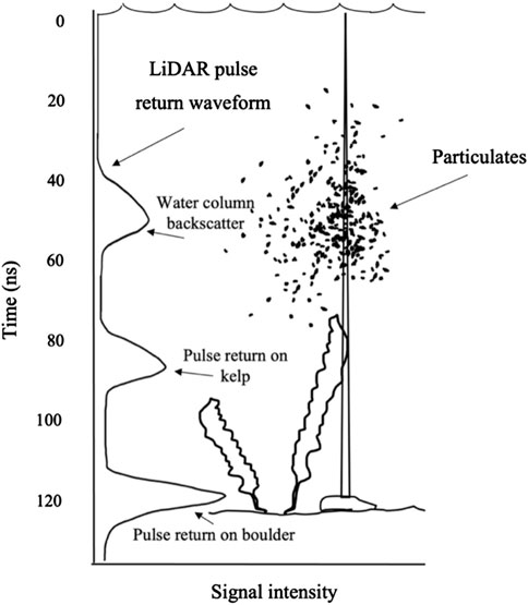
Figure 3. Pulse return phenomenology example in kelp underwater habitat, showing the pulse return waveform from T₀ near surface until T₁₃₀ nanoseconds and 1) return peak associated with water column backscatter from particulates (e.g., phytoplankton or inanimate/inorganic matter), 2) return associated with laser beam intersecting with kelp surface and 3) reflection off bottom boulder surface.

2.6 Lidar waveform processing

A simple form of full-waveform lidar pulse return “peak” processing via a serial line scan system is to detect the maximum pulse return intensity value within each pulse return waveform and subsequently recreate the imaged environment or substrate with these maximum values, point-by-point, as pixels (either in 2D or 3D space). Naturally, the full-waveform capacity allows the range gating of the point cloud data to effectively “image” a subsection of horizontal plane in the water, and peaks can be identified within a selected time frame or temporal slice (or distance) from the lidar. This pulse processing method (i.e., maximum peak intensity value) is adequate when operating in an aquatic environment with low surface heterogeneity where a single return is expected (e.g., bare sand or rock). Additionally, while not applied to our data, a possible way of optimizing processing speed and pulse peak processing is to select waveforms for peak processing only when signal waveform shows values above a certain noise threshold and observed peaks are of a certain duration (i.e., corresponding to the outgoing pulse characteristics) (Xing et al., 2019; Jutzi and Stilla, 2006). A different cut-off value can be chosen depending on the sensor characteristics and may help to eliminate false returns and lessen waveform processing time. This baseline threshold intensity can for example, be estimated and set slightly above the lowest intensity observed on a return waveform obtained from imaging a flat surface, in air, where the only thing interacting with the light pulse is the surface (not considering air molecules). The measured voltage intensity in absence of a substrate or particles would correspond to the detector’s lowest light intensity measurement. Peak detection is therefore more evident when the observed substrates are within lidar range to maximize the difference between peaks and lows or the baseline measurement.

Lidar data can be evaluated for depth or range by the following calculation, based on the speed of light on a laser pulse in seawater, and a return peak located 200 ns after pulse departure (T₀):

Speed of light: 299 792 458 m s⁻¹

Water index of refraction: 1.33

Speed of light in water: 225 407 863.158 m s⁻¹

Waveform pulse return location (i.e., in time, 1/2 light round trip): 200 $\mathrm{x}$ $\frac{1}{2}$ = 100 ns

Distance travelled by light in water (m): 100 E⁻⁹ s $\mathrm{x}$ 225 407 863.158 m s⁻¹ = 22.54 m

These measurements can later be attributed to return peaks within a waveform and recreate a “range” map of the imaged substrate, or 3D point cloud.

As the waveform represents a summation of the signal reflections or measurements (representing surfaces or objects at various proximities) after a lidar pulse, return peaks of interest may partially overlap within the waveform and be difficult to identify or differentiate. This can have the effect of reducing peak location positioning accuracy in time (and in space), and lower overall point cloud density. Waveforms may also require correction from the instrument electronic noise (i.e., how the electronics modifies the signal) or filtering out of the system impulse response, considering for the outgoing pulse width and amplitude to reconstitute a more accurate waveform (Neuenschwander, 2008; Wu et al., 2011; Wagner et al., 2006). The waveform can be described from the interaction of the following terms, in Equation 1 (inspired by Zhou et al. (2017)):

$P_r\left(t\right)={\displaystyle \sum _{i=1}^n}\frac{D^2}{4\pi {\lambda }^2{R}_i^2}{P}_t\left(t\right)*\tau \left(t\right)*{\delta }_i\left(t\right)(1)$

Where $P_r\left(t\right)$ is the laser power received or the intensity of the signal at a time index of $t$, $P_t\left(t\right)$ represents the outgoing pulse (its width and amplitude), $\tau \left(t\right)$ represents the system (or receiver) impulse function (width and amplitude), D the diameter of the receiver optics, λ is the laser wavelength, R is the range between the lidar and the target, δ_i $\left(t\right)$ is the cross section of the target (its surface area visible to the laser emitter) and n is the number of objects or locations with which the laser beam has had interactions. It is seen here how the outgoing pulse and system impulse function play a part in the received laser power.

This correction for system and imaging medium effects can be done in one or two steps, 1) Deconvolution, to remove the lidar system impulse response contribution to the observed waveform and 2) Gaussian Decomposition, which provides a method of locating observable and hidden peaks/pulse returns from the complex waveforms. For this work, deconvolution methods tested are RL and Gold’s algorithms, and waveforms were decomposed by the Gaussian method, using R package “waveformlidar” (https://github.com/tankwin08/waveformlidar) (Zhou and Popescu, 2019). Deconvolution and decomposition methods may be combined, by initially performing a deconvolution to facilitate Gaussian decomposition and return peak isolation. These methods will be presented in subsequent sections.

2.6.1 Waveform deconvolution

In the case of a more complex return waveform, deconvolution can be applied to effectively increase the difference between peaks and lows, better differentiate between peaks and thereby essentially increasing the SNR of the waveform and peaks in relation to the instrument and background noise, if the initial SNR is above the noise threshold. Since light travels at 0.3 m ns⁻¹ in air, or 0.225 m ns⁻¹ in salt water, optimizing the pulse return waveform of the lidar can help optimize range resolution.

As described in Zhou et al. (2017), the successive deconvolved waveform can be estimated from an observed signal, $d\left(x\right)$ at time $x$, by iteratively convolving (*) the current estimate of the waveform, $f_t\left(x\right)$, with the point spread function (PSF), $g\left(x\right)$. The PSF includes both the system impulse response and the outgoing pulse interaction. The deconvolution can be expressed as in Equation 2 (Fish et al. 1995):

$f_{t+1}\left(x\right)=f_t\left(x\right)\left(\frac{d\left(x\right)}{f_t\left(x\right)*g\left(x\right)}*g\left(-x\right)\right)(2)$

In discrete form, the RL algorithm can be expressed as in Equation 3:

$x_k\left(i\right)=x_{k-1}\left(i\right){\displaystyle \sum _{l=1}^n}\left[\frac{y\left(l\right)}{{\sum }_{j=l}^{n}h\left(l-j\right)x_{k-1}\left(j\right)}·h\left(l-i\right)\right](3)$

where $x_k\left(i\right)$ is the estimate of the original signal at iteration k and time bin $i$, $y\left(l\right)$ is the measured waveform at time bin $l$, $h$ is the system impulse response, and $n$ is the total number of time bins.

Comparatively, Gold’s algorithm can be described as follows in Equation 4 (Morháč et al. 1997):

$x_k\left(i\right)=x_{k-1}\left(i\right)\frac{y\left(i\right)}{{\sum }_{j=1}^{n}h\left(i-j\right)·x_{k-1}\left(j\right)}(4)$

Here, Equation 4 $x_k\left(i\right)$ and $x_{k-1}\left(i\right)$ are the current and previous estimates at time bin $i$, respectively, $y\left(i\right)$ is the measured waveform, and $h\left(i-j\right)$ is the system impulse response at time bin $i-j$.

More concisely, knowledge of the 1) Iidar’s outgoing pulse is required (FWHM, or the pulse width from start to end of peak), 2) system impulse response, which in this case is how the optics and electronics possibly reshape the pulse as it reaches and interacts with the target surface, and is recorded by the lidar digitization hardware. This can be done for example, by sending and receiving a pulse on a single reflecting surface, at nadir. The outgoing pulse and system impulse response can thereafter be used for deconvolution of the observed return signal. For more detail, the user can be directed to see the R package waveformlidar and Zhou et al. (2017) for additional details on the methods.

2.6.2 Waveform decomposition

Environments where vertical structure composed of eelgrass, macroalgae/kelp or coral is present often have more complex vertical profile and can benefit from a more optimized pulse return peak detection in producing more representative 3D point clouds. A common method is to use Gaussian Decomposition, from the understanding that a lidar waveform can be described as a sum of Gaussian pulses (Wagner et al., 2006). Each pulse return waveform is analyzed for the presence of peaks (i.e., algorithm dependent on the type of signal, if noisy) and their characteristics (height, width, and location (i.e., time-of-flight)) are noted. The resulting waveform f(x) (Equation 5), composed of this sum of Gaussians can be described as:

$\mathrm{f}\left(\mathrm{x}\right)={\displaystyle \sum _{k=1}^n}{\mathrm{A}}^k\exp \left(-\frac{{\left(x-u_k\right)}^2}{2{\sigma }_k^2}\right)(5)$

where n is the number of Gaussian elements identified after deconvolution done in the previous step (Section 2.6.1.) for each waveform via a peak finding algorithm, A^k represents the amplitude of the identified peak k, within the waveform, u_k is the location in time of the peak, and $\sigma$ is the standard deviation of the same peak. Additionally, a mean filter can be applied to each waveform processed by decomposition to attenuate signal noise, the latter affecting how pulse return peaks can be detected.

3 Results

3.1 Lidar pulse return analysis and phenomenology

3.1.1 Sand and eelgrass

The main identifiable pulse return waveform features when imaging eelgrass patches (Figure 4a) are in 1 image-bearing forward scatter associated to the sandy bottom (high peak, Figures 4b,c) (single peak)), 2) image-bearing forward scatter from bottom substrate (highest peak) and sparse eelgrass canopy (middle bump at time interval 40–60 ns, Figure 4d), and 3) low-amplitude common volume back scatter (waveform section preceeding middle bump, at time interval 0–40 ns, Figure 4d). Coming from a near-monostatic lidar system, the PMT sensor field of view is wide enough that the common volume backscatter reception is possible. The waveforms are however not showing signs of this middle bump, and we can interpret that it is most likely not multiple backscatter, nor common volume backscatter. Eelgrass blades positioned just above the benthic substrate and reflecting towards the lidar are likely the cause of the increased signal intensity (i.e., at 40–60 ns) preceding the high peak return from the bottom sandy substrate. A “double” peak observed at 70–75 ns in Figure 4e) likely represents the intersection of an eelgrass blade (or other object occluding the bottom substrate partially) by the laser beam, a moment before the residual laser pulse reaches the bottom substrate.

Figure 4

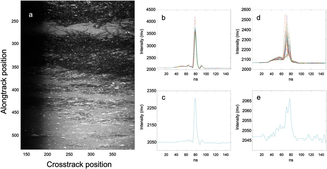
Figure 4. Shallow Pointe-Lebel seagrass site, (a) eelgrass and sand transect, interspersed with small shells and pebbles, (b) 40 waveforms from line 500 and rows 200:240 over sand, (c) single waveform from line 500 and row 210 over sand, (d) 40 overlapping waveforms from line 300 and rows 200:240 over eelgrass and sand, (e) single waveform from line 300 and row 210 over eelgrass and sand.

3.1.2 Macroalgae and intermixed coral (shallow)

The Florida - Erojacks site displayed several macroalgal and coral substrates over a sandy bottom, where the coral is found in either upright or encrusting form. The elastic lidar channel performed as expected, whereas the inelastic channel was troubled by a circuit-related power variation and made use of images and point cloud data challenging in most cases (but not individual waveforms). In the context of imaging with both elastic and inelastic channels, main identifiable pulse return waveform features when imaging macroalgae intermixed with coral are seen in Figures 5a,b and are 1) elastic image bearing forward scatter associated to the sandy or rock bottom (right peak), 2) elastic image bearing forward scatter from macroalgae/coral target (left peak), 3) very low volume backscatter (waveform section preceding the two peaks). Further, the observed waveform does not show any multiple nor common volume backscatter. Coincident water visibility conditions were good to very good. Additionally, inelastic and image bearing backscatter is also visible in the inelastic channel acquired waveform and shows two return peaks. When these two imaging channel waveforms are placed one over the other, it is apparent that the left peak is associated to a vertical structure capable of fluorescence (Figures 5c,d), and the right peak corresponds to the bottom substrate, which also has an observable fluorescent signal, albeit less intense when covered by a vertical structure.

Figure 5

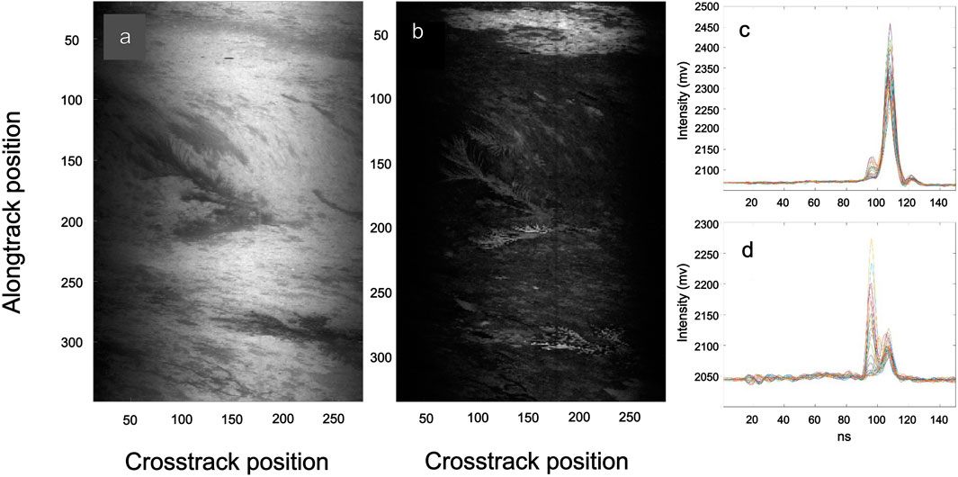
Figure 5. Shallow (10–20 ft) Erojacks reef site - left, (a) elastic (532 nm) and (b) inelastic (685 nm) images showing macroalgae and coral transect over sandy bottom substrate near Erojacks site, Dania Beach, FL, United States, (c) 30 elastic and (d) 30 inelastic waveforms from line 200 and rows 120:150 over macroalgae and sand/hard substrate.

3.1.3 Coral reef (deeper)

Based on several reconstructed 3D point clouds taken during West-East transect sections over Barracuda Reef, macroalgae and corals were present and observed over a reef/rock under structure. Supported by Secchi disk depth measurements of 5.5–6.0 m taken while the ship and imaging system were immobile, overall pulse return history shows a clear water column by the lack of elastic backscatter associated to the water column (Figure 6). This sea trial also used both optical channels for elastic imaging and detection (i.e., no fluorescence). Some of the nearfield waveform data shows backscatter caused by water surface turbulence and air bubbles caused by the ship propeller cavitation, the ship hull contacting the water surface as well as surface wind and wave action. Surface to reef distance varied from 15 to 25 m.

Figure 6

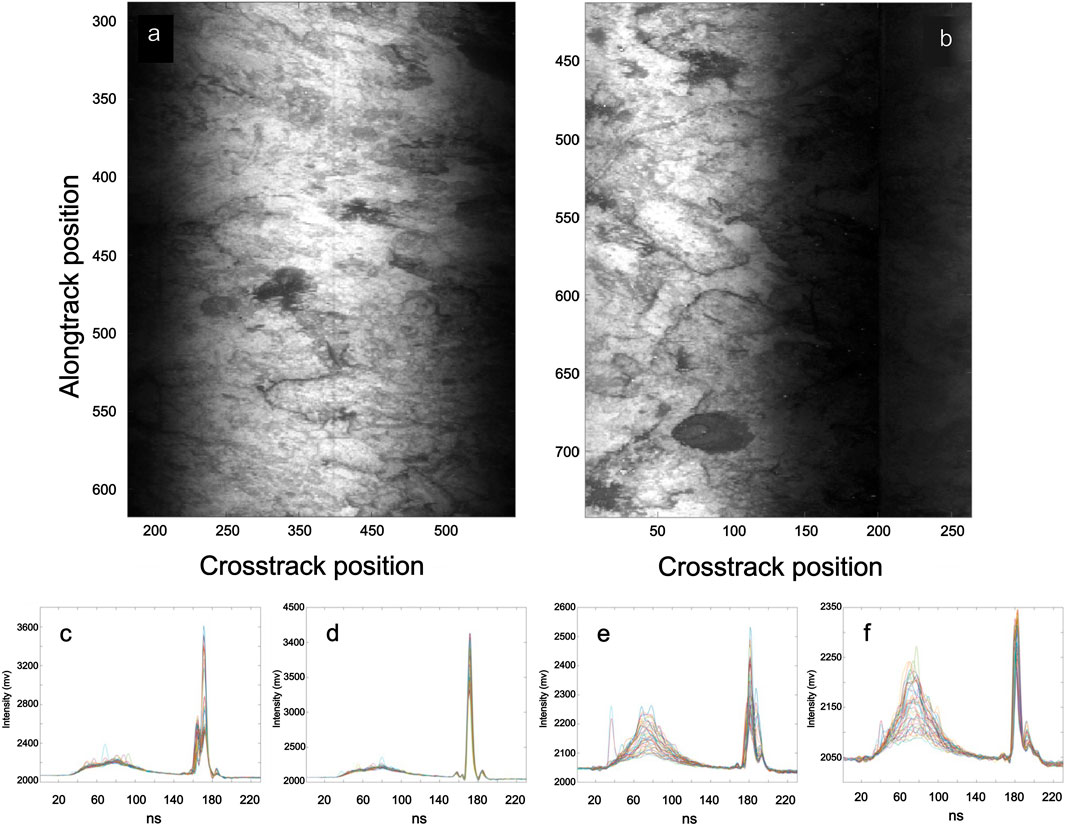
Figure 6. Deep (50–70 ft) Barracuda reef - above left, (a) elastic (532 nm) and right (b) elastic (532 nm) images showing macroalgae, possibly coral and hard bottom/sand substrate over Barracuda Reef, Dania Beach, FL, United States; (c) 40 elastic waveforms from line 475 and rows 270:310 over macroalgae and sand/hard substrate, (d) 40 elastic waveforms from line 440 and rows 270:310 over sand/hard substrate; (e) 40 elastic waveforms from line 450 and rows 80:120 over macroalgae and sand/hard substrate, (f) 40 elastic waveforms from line 450 and rows 80:120 over unknown dark substrate (possibly biological in nature).

3.1.4 Macroalgae/kelp over boulders/rocks

As water turbidity was relatively high on the lidar transect survey in Godbout area, it is difficult but possible in some cases to show kelp in bottom images (Figure 7). However, dive surveys performed 2 days before showed an extensive kelp stand over a rock and boulder substrate. Common volume backscatter is clearly visible as a “bump” on the left of waveforms, on both elastic and inelastic channels of Figures 7d–g sub-images. This is likely because fluorescence in the backscatter of the inelastic waveform images was not detected due to reabsorption (i.e., by other Chl-a containing cells such as phytoplankton) and scattering processes within the turbid water column. Elastic waveforms of kelp stipe Figure 7d show several distinct peaks besides the common volume backscatter, where the rightmost peak corresponds to the sea bottom. Comparatively, Figure 7e shows waveforms where the kelp blade surface is considered to be where the maximum peak is located and only a very low subsequent peak is seen, likely since the kelp blade intercepted most of the light. This may also be a false peak and associated with the detector signal response. The inelastic waveforms confirm the presence of fluorescence response at the rightmost peak, likely kelp from the supporting images at the top left, and a weak bottom peak slightly deeper than the depth at which the kelp blades are found. Further, although not visible in actual bottom images (i.e., not shown), there are numerous occasions within the dataset showing presence of peaks associated with fluorescent surfaces in line with the elastic image peaks. The fluorescence backscatter associated to these inelastic signal peaks is likely not visible due to surrounding image noise (and signal variability) generated by particulates in the water column. These peaks would however show up in the 3D point clouds and contribute to the construction of an underwater kelp/macroalgae canopy or rock surface. They would however require additional peak processing to properly locate and characterize them (i.e., amplitude, width, position in time) amongst the noise. Although the images recomposed from the Godbout lidar scans in Figure 8 do not reveal any structures because of water turbidity and deeper bottom (images not shown), waveforms show underlying surface reflections (i.e., pulse return peaks) that can reconstruct a 3D point cloud.

Figure 7

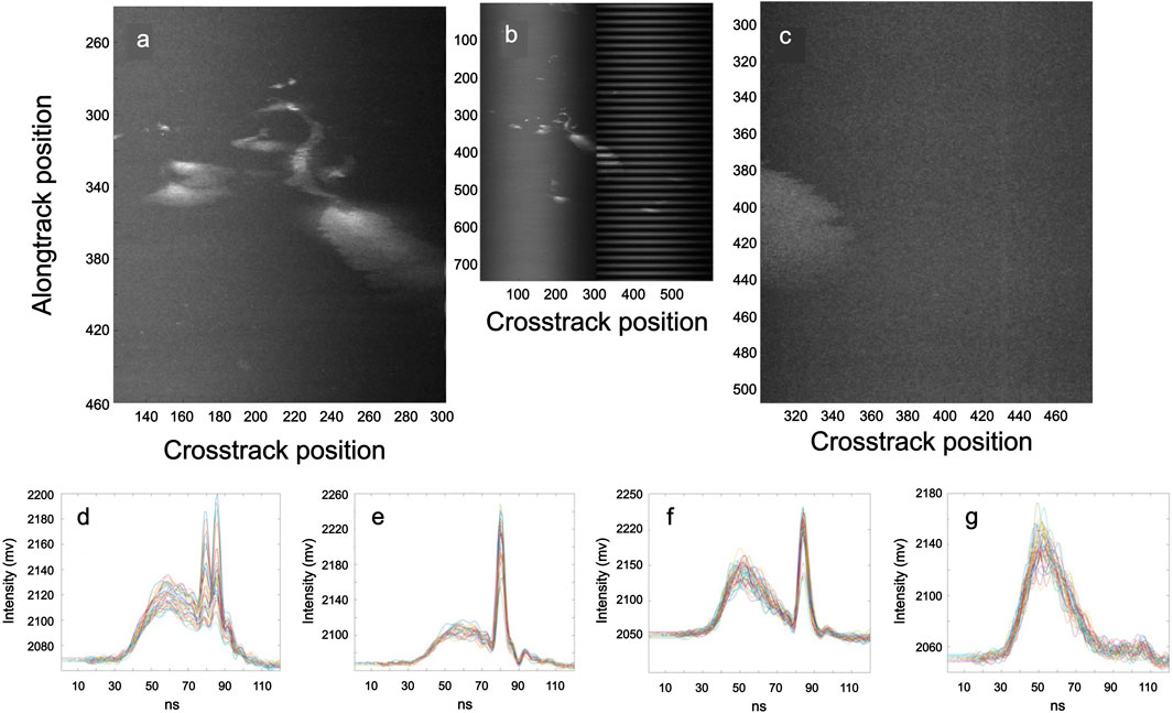
Figure 7. Lidar images of (a) kelp closeup - elastic, (b) entire elastic image, (c) fluorescence image showing kelp blade as seen by the fluorescence channel, (d) kelp stipe area at line 332 and rows 215 to 255, with common volume backscatter (left bump), and multiple peak returns (right), (e) elastic waveforms at line 360 and rows 240 to 270 show elastic but single returns on apparently flat kelp blade, preceded by common volume backscatter, (f) inelastic returns at line 400 and rows 305 to 345 associated with the water column backscatter and with the backscatter associated to the kelp blade, represented by the single sharp peak and (g) waveforms at line 300 and rows 305 to 345 show inelastic backscatter associated with the water column where no kelp or other target surface is seen on the lidar image, but a weak pulse return peak near 100–105 ns associated with the bottom can be observed.

Figure 8

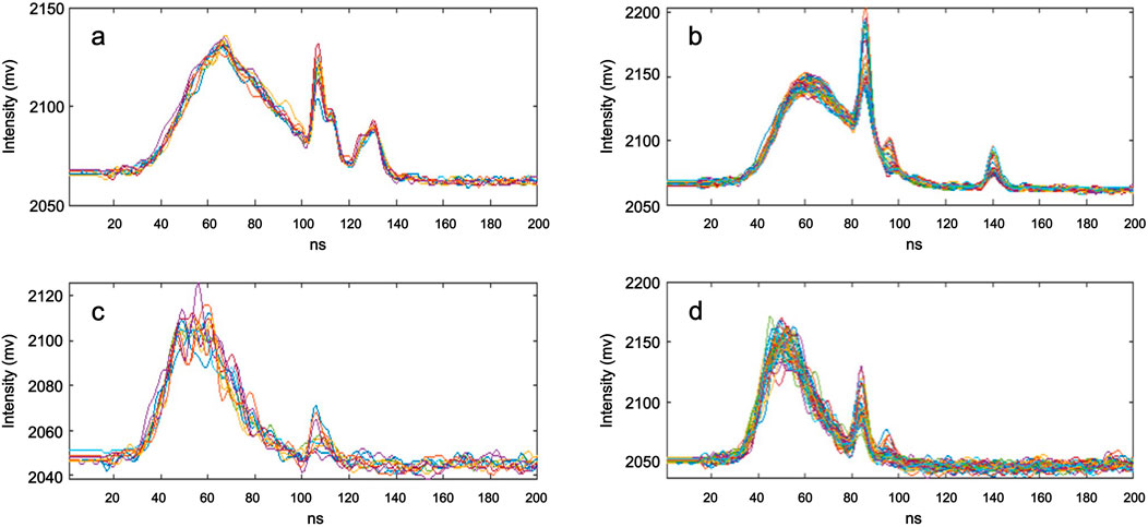
Figure 8. Lidar pulse returns showing multiple peaks of varying signal intensity and showing high water column backscatter (a,b) elastic, (c,d) inelastic) in turbid waters, Godbout, QC, Canada.

Another common substrate in the Godbout area that is likely to be colonized by kelp are rocks/boulders, in this case varying in size from 10 cm to 100–200 cm in diameter (as observed), interspersed over a sand substrate (i.e., less visible when many boulders/rocks are present). The observed waveform pulse returns over boulders appear characteristic of hard and highly reflective substrates (Figure 9). Figure 9c shows a lessening of the return energy as the laser scan moves away from the top of the boulder to its right side, where light is believed to be increasingly diverted sideways, reducing the amount of light reaching the detectors. The common volume backscatter is present, although much less important than the boulder signal even though the boulders are located at depth. Waveforms associated to the side of the boulder show additional peaks (Figure 9c), likely from a reflection of the initial pulse hitting the boulder/rock, or perhaps a short vertical object/structure present on the rock substrate (e.g., algae). This is however not apparent in fluorescence image channels.

Figure 9

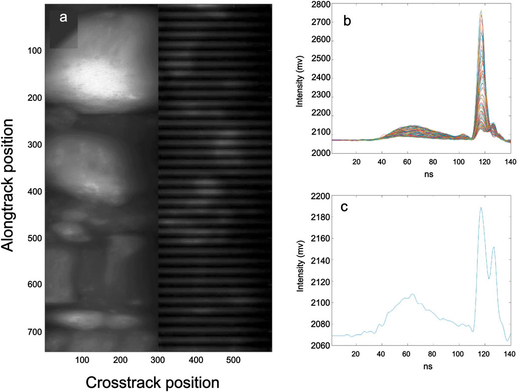
Figure 9. Elastic lidar image in boulder field (a), and (b) associated pulse returns of varying intensity in the boulder center to its right edge, at line 350 and rows 180–290, and (c) bottom right-side of boulder at line 350 and row 290 in turbid imaging conditions, near Godbout, QC, Canada.

3.1.5 High turbidity - no detectable bottom

Attempts to acquire multi-species and color class macroalgal dataset in Matane, QC, Canada were unsuccessful due to high turbidity during the 2-day survey time window. Depth at the time of the survey was approximately 5 m and with a measured Secchi depth of 2.9 m. A reconnaissance underwater ROV video transect done prior to the lidar transect survey showed macroalgae of various species in the 5–40 cm height range. The main and only feature visible on all data acquired is water column backscatter and it shows an important contribution of suspended particulates to backscattering of the signal (Figure 10). Moreover, we can see the approximate time-distance at which the laser pulse passes through the acrylic housing, and it corresponds to the distance travelled from laser pulse initiation to the acrylic-water interface. Further, the common volume backscatter appears to have two amplitude components, one with higher intensity values starting near T = 17 ns, and the other with lower intensities and weaker slope at T = 19 ns This can be attributed to the two elastic optical channels having a slightly different angular response and gain setting at the time (i.e., prototype phase) more so than variations in turbidity along the scanned transect line, although the latter is possible.

Figure 10

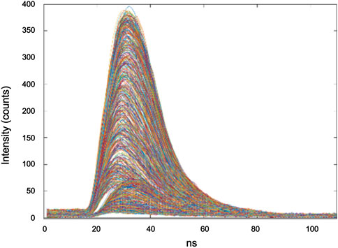
Figure 10. Water column backscattering visible from lidar transect at high water column turbidity, Matane, QC, Canada. Overlapping waveforms shown in the figure correspond to pulse returns recorded from a single line of transect.

3.1.6 Deconvolution applied to pulse return waveforms

The waveform samples taken in shallow eelgrass habitat and coastal macroalgae and coral reef both show relatively little effect of common volume backscattering, in part due to relatively optically clear water conditions, as well as short range imaging (Figures 11, 12, a and c). Common volume backscattering is more noticeable via the deep coral reef habitat data (Figures 13a,c), but effects are somewhat limited in terms of image degradation (see previous section for images of bottom reef substrate) and benthic lidar return signal is strong. This represents a long imaging range for the present lidar system (nearly 20 m) and is expected in clearer waters further away from shore. Comparatively, imaging of kelp in Godbout, QC, Canada, was much more affected by the backscattering due to post-storm high turbidity water conditions (Figures 14a,c). This had the resulting effect of reducing imaging contrast (i.e., previous section, kelp images).

Figure 11

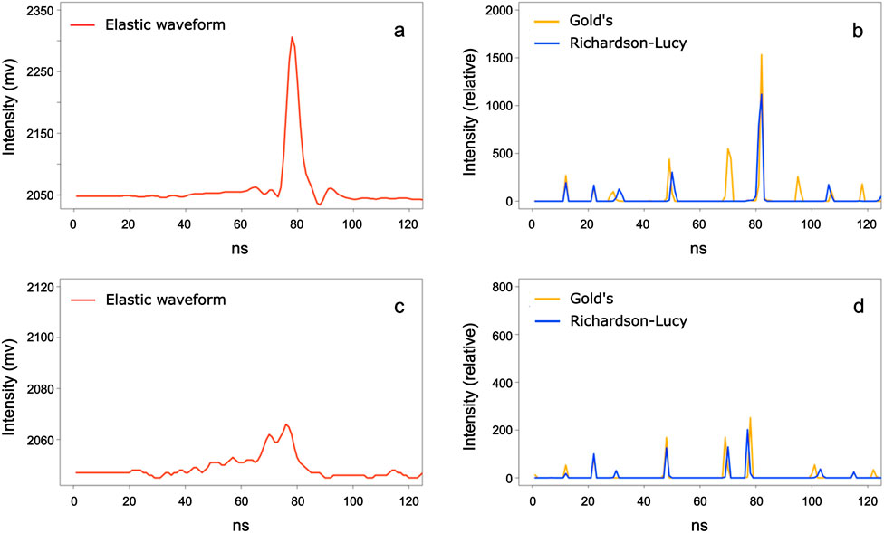
Figure 11. Eelgrass and sand lidar pulse return waveform peak processing example, showing unprocessed raw (a) elastic and (c) elastic pulse return waveforms, as well as resulting deconvolved (b) elastic and (d) elastic pulse return waveforms using Richardson-Lucy (blue) and Gold’s algorithms (gold) deconvolution algorithms. The fluorescence (inelastic) sensor was not used in this specific imaging trial, hence the two elastic waveforms.

Figure 12

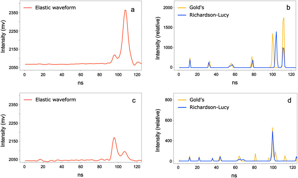
Figure 12. Macroalgae and coral lidar pulse return waveform peak processing example, showing unprocessed raw (a) elastic and (c) inelastic pulse return waveforms, as well as resulting deconvolved (b) elastic and (d) inelastic pulse return waveforms using Richardson-Lucy (blue) and Gold’s algorithms (gold) deconvolution algorithms.

Figure 13

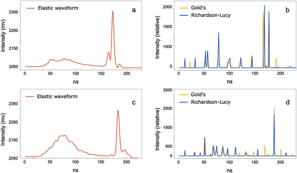
Figure 13. Deep reef (Barracuda Reef, FL, United States) macroalgae and coral pulse return waveform peak processing example, showing unprocessed raw (a) elastic channel A and (c) elastic channel B pulse return waveforms, as well as resulting deconvolved (b) elastic channel A and (d) elastic channel B pulse return waveforms using Richardson-Lucy (blue) and Gold’s algorithms (gold) deconvolution algorithms.

Figure 14

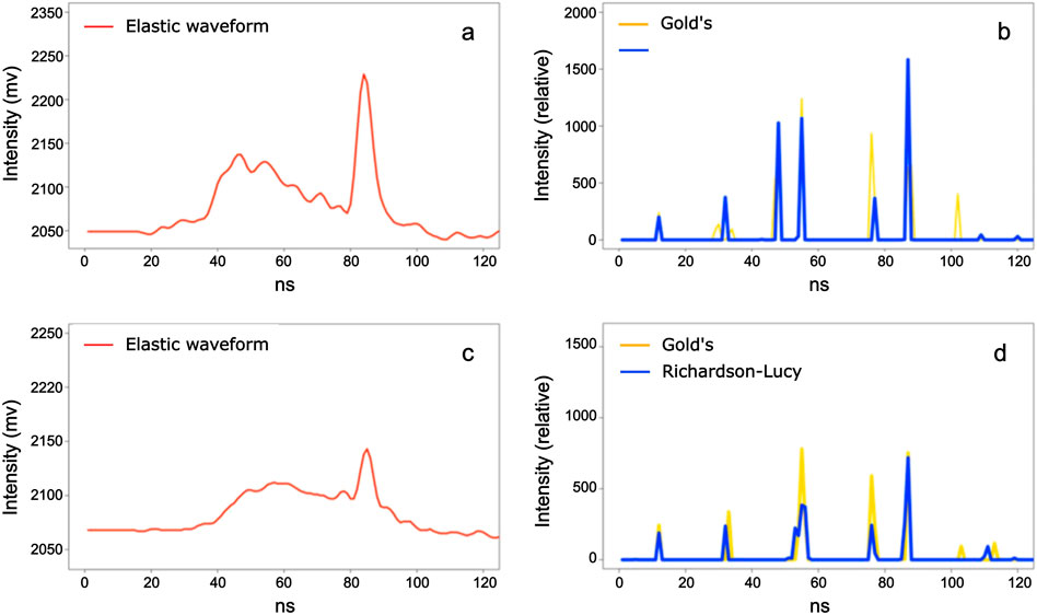
Figure 14. Kelp species Saccharina latissima lidar pulse return waveform peak processing example, showing unprocessed raw (a) elastic and (c) inelastic pulse return waveforms, as well as resulting deconvolved (b) elastic and (d) inelastic pulse return waveforms using Richardson-Lucy (blue) and Gold’s algorithms (gold) deconvolution algorithms.

Both deconvolution methods applied to waveform samples in the eelgrass habitat proved efficient in making pulse return peaks associated to the sand and eelgrass substrate more evident in the case of where there was eelgrass (Figures 11c,d), where signal strength was much lower than on the sand substrate (Figures 11a,b). Although there appears to be an additional return peak mid-travel in the second deconvolved elastic waveform (c), it may represent mid-water column substrate such as an eelgrass leaf or be part of the signal noise. The former is more likely in this case, since the optical channel was set to elastic (not fluorescence) for this trial, and noisier waveform was observed more so in inelastic or fluorescence measurements as the observed fluorescence intensity can be closer to the electrical background noise. Moreover, a higher threshold for signal noise should be set when the waveform signal is noisy (i.e., fluorescence measurements) to reduce the number of falsely detected peaks.

The same type of efficient peak identification result is observed for the macroalgae and coral waveform dataset. In this example, the elastic return (Figure 12a) on hard and reflective substrate can be isolated with both deconvolution methods, but Gold’s seems to retain the additional peak located just before the main peak, and the position and relative intensity are better maintained as well. Comparatively, only the Gold’s method was able to discern the two pulse return peaks on the inelastic fluorescence channel (Figure 12c), whereas the RL algorithm discerned a single peak.

Deep water coral reef waveforms (Figure 13) further demonstrate the applicability of deconvolution algorithms, and it is apparent that Gold’s algorithm has isolated more peak returns. This is also apparent in the former two imaging scenarios, as well as the macroalgae–kelp imaging trial (Figure 14). Moreover, considering that Gaussian decomposition cycles through these deconvolved waveforms to identify peak return locations, widths and amplitudes, decomposition should be done respecting a certain threshold value for the pulse return peaks identified through deconvolution. These results demonstrate the variable nature of lidar pulse return waveforms and the necessity to fine-tune data processing parameters, per situation, for optimal peak identification, characterization, and subsequent 3D point cloud reconstruction.

3.1.7 Decomposition applied to pulse return waveforms

If waveform deconvolution processing was needed and/or it is done to enhance pulse return peak resolution within a more complex waveform, decomposition is now applied to this waveform to determine the location of peak returns more precisely within each waveform. The peak location and amplitude data can then be used to construct the 3D point cloud “pulse-by-pulse”. In this context, we show an example of Gaussian decomposition on a pair of corresponding elastic and inelastic waveforms, either in their raw form or following RL and Gold’s algorithm deconvolution, with the macroalgae and coral datasets (see Figure 12 for reference to the waveforms). Peak identification and characterization done on this data are shown in Table 2.

Table 2

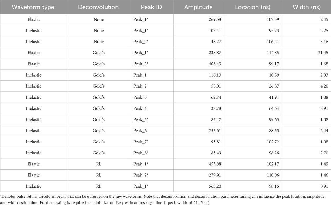
Table 2. Example of lidar pulse return waveform peak amplitude and location identification in data acquired over macroalgae and coral substrate (see Section 3.1.2 for figure reference), either in unprocessed format (i.e., no deconvolution), or deconvolved using Richardson-Lucy (RL) and Gold’s (Gold’s) algorithms.

Decomposed waveforms may sometimes suggest some form of initial signal smoothing to be applied to raw, sometimes noisy waveforms (i.e., low low-intensity signal). For example, a noisier waveform (see Figures 12c,d) will create more false peaks associated to the variations in signal intensity, as seen in the decomposition results using Gold’s algorithm on the inelastic waveform (Table 2). The algorithm effectively enhances multiple peaks within the noisy waveform section preceding the main peaks. In this case, the use of the peak parameter probability values (i.e., amplitude, location-time, width) that are provided in the decomposition results (available in the R ‘waveformlidar’ package but not shown for brevity), can further guide in selecting the final peak(s) and associated parameter value(s) for reconstructing the 3D point cloud.

A signal threshold value by which to decide whether to apply deconvolution and/or decomposition on some segments of the waveform should help mitigate potential false returns as well, especially when optimizing peak detection in inelastic waveforms where a lower SNR usually characterizes this optical channel, and that detected fluorescence signal intensity is generally closer to the instrument electronic noise level than the reflectance channel. Additionally, although deconvolution can have the effect of changing the detected return peaks’ amplitudes, this can be corrected for example, by rescaling deconvolved peaks to the original waveform amplitude characteristics or by using only the deconvolved peak locations and fitting them to the original waveform with true signal amplitude measurements. Furthermore, additional decomposition and deconvolution parameter tuning should be considered to avoid erroneous estimates (e.g., Table 2, line 4: peak width of 21.45 ns that should be much narrower). However, in the context of processing a larger 3D point cloud with many thousands of peak returns and waveforms, such errors may be evened out or considered as outliers, not affecting the overall substrate reconstruction process.

4 Discussion

Large-scale and high-resolution shallow coastal underwater benthic surveys are necessary for the current and future to monitor coastal environmental resources (e.g., from resource exploitation, man-made habitat disturbance) and overall biodiversity, as well as in relation to climate change scenarios. In situ underwater laser line scan-based and lidar remote sensing offer advantages by integrating the spectral response of surfaces and live organisms for additional levels of remote, automatic classification and characterization, while offsetting some of the setbacks associated to imaging for habitat characterization in coastal waters (i.e., visibility). Our study is among the first besides continuous-wave laser-line-scan underwater imaging studies (e.g., Huot et al., 2023; Huot et al., 2022; Strand et al., 1997; Mazel et al., 2003) to demonstrate the capabilities of underwater lidar fluorescence for imaging and detection of biological ecosystem components including kelp and other macroalgae, coral, eelgrass in their natural habitat and associated bottom substrates. Further, we developed on the possibilities of expanding full waveform lidar signal processing methods to the underwater environment, providing a comparison between habitats and substrates while highlighting the main particularities associated to the environment, substrates, and imaging methods.

4.1 Habitat-dependent lidar pulse return characteristics

The pulse-return waveforms associated to underwater benthic substrates observed in this work can be characterized as of medium to low complexity, by the relatively low number of peaks per return waveform generated by the small beam footprint (Shan and Toth, 2018) and low signal noise component. This can be in part due to the studied surfaces themselves, and/or how the laser beam is set to interact with water column and benthic structures being present. When large, whole and/or thick surfaces are first hit, they are likely to allow less or no multiple returns from the laser pulse interacting with other nearby surfaces below and past the initial surface. However, a fraction of the incident photons may be transmitted through the initial surface or reflected onto another in proximity and generate one or more pulse returns associated to the initial pulse. Whether this is a frequent outcome is to be determined but could increase the density of elastic and inelastic 3D point clouds where the light attenuation properties (i.e., absorption and scattering) of the water allow sufficient transmission of light from reflections or fluorescence for it to be detected. This biologically related pulse time-history phenomenon of multiple reflections and stimulated fluorescence emissions could be more present in the Godbout (kelp) dataset but would be dependent on the presence of highly reflective surfaces. The latter may or may not always be common in an underwater setting where epibionts (e.g., epiphytic algae, diatoms) can cover the blade and stipe surfaces (Teagle et al., 2017), especially near the end of a growing season when structures are becoming senescent and/or in conditions that may promote the growth of the epibionts (e.g., higher temperatures, high nutrients) (Andersen et al., 2011).

Comparatively, the horizontal cross-section through a patch of eelgrass viewed from above as in the Baie-Comeau, QC, Canada dataset, will be much more transmissive or rather allow for parts of the incident laser pulse to interact with different substrate layers in its path, if present, causing reflections and fluorescence (when fluorescent capable substrate is present). A likely characteristic of this is that return peaks associated to a 3–4 mm wide eelgrass blade at its widest (i.e., or less if not perpendicular to the incident beam), may be of lower intensity than in the case of a surface encompassing the entire laser beam footprint (e.g., 10 mm diameter circle), as less light is detected per reflection event. Several eelgrass surfaces of similar cross-sectional area may be along the laser pulse’s path and lead to multiple returns within a short distance, which may be more difficult to discern from one another without waveform deconvolution and decomposition processing. Multiple nearly overlapping peak returns can also be expected in corals if fine branching structure is present, and any other type of macroalgae. This was not directly seen within the context of these trials, but while this fine structure may be less present in larger kelp, multiple returns can also be obtainable from the same specimen in different parts of the structure, such as in the Godbout, QC, Canada (kelp) dataset where multiple stipes are seen and show this feature in the corresponding waveforms.

Waveform peaks were observed in both elastic (reflectance) and inelastic (fluorescence) waveforms in most field trial situations described. Some of these peaks may have been formed in part from the “ballistic” component (Yoo and Alfano, 1990; Tanner et al., 2017) of the reflected or emitted light, which is constituted by photons that have not been scattered and have otherwise travelled in a straight line from the reflection or emission event. Comparatively, waveform peaks can also be formed from the contribution of “snake” photons, which are those that have been deviated (as in a snake making its way forward, indirectly) from their initial trajectory by a few direction changes, after reflection, or emission, but have managed to make their way to the optical receiver. These could be potentially differentiated and compensated for, by the timing of their arrival at the optical receiver, and logically, may cause the waveform peaks to be wider in more turbid imaging conditions from the additional interactions in the water column.

Besides energy density, another advantage of using small laser footprint is the possibility of generating high resolution images from near-overlapping pulses. Hence, the instrument is also useful in acquiring images for additional spatial and shape features potentially useful for substrate type classification. Using a larger laser footprint size, as would often be done in terrestrial or aerial lidar detection, would allow to cover more surface area (Collin et al., 2011) but generally require much more powerful lasers for canopy penetration than are typically useable for underwater AUV purposes (i.e., reasonable power requirements, weight). The benefit of a larger beam footprint is a larger scanned area during a survey, but the tradeoff is a reduction in resolution limited to the footprint size, blending fine substrate features and detail (e.g., substrate border features, color, texture, spectral response) useful for more precise substrate classification.

The consequences of working in water are that light absorption and scattering are much more present and are responsible for attenuating the laser beam energy as it travels through water. As the objective in designing a fluorescence capable lidar is also to generate as much fluorescence as possible for detection but also imaging, the laser beam footprint must be relatively small to avoid lowering the energy density and maintain fine surface features but not limit scan area coverage excessively.

The phenomenon of continuous and pulsed laser absorption and scattering processes in the water column have been described in previous studies (e.g., Mullen et al., 2013; Strait et al., 2018), and for which results directly apply to this pulse time-gated instrument design. In these studies, scattering agents such as Ultra-fine Arizona test dust and Barium sulfate were effectively applied at different concentrations to test image contrast and resolution, and show that contrast limiting attenuation length of approximately 5–6, possibly 7 can be reached with the current system (e.g., Dalgleish et al., 2009). This can be used to predict imaging performance in specific working environments where turbidity can be initially measured, and adjust sampling methodologies (i.e., distance to substrate, imaging wavelengths). Consequently, elastic lidar returns will be more effective for substrate detection and 3D point cloud creation in more turbid waters than fluorescence returns because of the return signal attenuation from the higher absorption of longer wavelengths in water (Mobley, 1994).

4.2 Adjusting 3D point cloud spatial resolution via signal processing

Waveform processing methods - RL and Gold’s algorithms - both improved waveform interpretability noticeably in providing more well-defined pulse return peaks and fully use the lidar’s sub – 3 ns – pulse duration to a high range resolution estimation. Chosen in part for their long-proven performance (i.e., RL) and/or for their recent (Gold’s) applicability to lidar pulse return signal processing, multiple other deconvolution (and decomposition) methods can be applied to various degree (and accuracy) and suitability is dependent on the data being treated (Zhou et al., 2021). Overall, Gold’s algorithm identified additional peak returns vs. RL’s, the former being possibly more sensitive to waveform variations. In hindsight, the deconvolution method used will likely be varied from one survey or substrate category to another, depending on the environment. Additionally, although the shown methods did increase peak resolution, deconvolution parameters are also adaptable, as is waveform signal smoothing, for avoiding identification of false returns. For example, comparing the mean noise of a waveform’s amplitude to the standard deviation of the mean noise can be used to detect false peaks (Zhou et al., 2021; Hofton et al., 2000; Parrish et al., 2011). Parameter selection for deconvolution, including iterations and repetitions, was determined by directly comparing raw waveforms with their deconvolved counterparts to assess the impact on peak clarity and localisation on the range (or time) axis. Rather than relying on fixed values, we examined how varying these parameters influenced waveform structure. Notably, the outgoing pulse and system impulse response appeared to have more direct effect on isolating peaks and accurately detecting their original locations in the raw waveforms. Assessment of these deconvolution approaches should be further investigated on more complex waveforms, within a more controlled environment such as with varying turbidity and absorption characteristics. Additionally, using by cross-validation techniques, one could apply deconvolution parameters for a specific application or imaging environment after having evaluated the performance of these parameters on the identification of pulse return peaks in waveforms of differing complexity.

These resolution enhancing methods are necessary for detailed benthic substrate studies, for example, biomass estimation in ecosystem service providers such as kelp and other macroalgae, corals, and eelgrass. Using the 3D point clouds to generate substrate or structure volume estimations, establishing the relationship between wet (live) biomass of these structures and the 3D volumes occupied in the water column can be validated on several specimen substrates in a controlled environment (e.g., experimental tank) and in the field. The presence of false pulse return peaks within the 3D point cloud in the vicinity of real returns might not have a large impact on the rendering of the data in 3D but should make it fuller in a sense. Further, erroneously identified lidar peak returns can potentially be removed from the final data by considering the probabilities associated to neighboring values or presence/absence of peak returns (or points) within this 3D volume (Ma et al., 2020). For instance, density-based algorithms for discovering clusters or groups within the point cloud data can be applied to the data in question (Ester et al., 1996; Zhang and Kerekes, 2015; Bryant and Cios, 2018).

4.3 Conclusion

As a natural evolution of lidar bathymetry, underwater lidar detection and imaging can be efficiently applied to semi-autonomous and autonomous biological underwater surveys using reflectance and fluorescence techniques. This study is among the first to describe underwater lidar pulse return phenomenology in habitat structuring biological substrates such as kelp and other macroalgae, eelgrass and corals. Moreover, the use of stimulated fluorescence emission as a means for remote sensing detection is shown to carry sufficient spectral response for detection as well as imaging at AUV-related operating distance, thereby providing additional means for addressing coastal environmental surveys at larger spatial scales and in timely manner. Further, data acquired in clearer waters and at close range are less likely to be affected noticeably by water column signal attenuation and dispersion effects and should allow pulse returns peaks to be more clearly separable and identifiable. These results further suggest the usefulness of autonomous underwater vehicle benthic surveys for remaining closer to the imaging substrates or targets of interest.

In the context of 3D point cloud generation, our study suggests that optimizing the number of detected pulse return peaks can be done efficiently via deconvolution and decomposition methods, as per methods shown and previously developed for other environment types (e.g., terrestrial). However, as these optimization methods can be processing intensive, substrate vertical and lateral complexity (e.g., branching, multi-layered structures) can likely predict the requirements for pulse return optimization and recognizing this feature could be integrated into the data acquisition and pre-processing steps. Another interesting approach for analysis of lidar waveforms for multiple returns is with neural networks and deep learning methods (Aßmann et al., 2021; Liu and Ke, 2022), and we should see some evolution of this approach in the coming years.

As laser and sensor technology adapted to underwater use evolve (e.g., other laser wavelengths, multi- and hyperspectral sensors), it will be possible to acquire data that can lead to enhanced detection of different spectral responses (e.g., acquired via multiple fluorescence optical channels), better identification and classification. Methods tailored to extract information from these increasingly complex multidimensional datasets such as those presented above will have to follow. In the context of characterizing and assessing the diversity of underwater biological substrates, structures as well as their habitat and environment, improving our understanding of light interactions on biological substrates via continuation of controlled experimental approaches will inform us as to how certain conditions may facilitate or limit certain optical phenomena (e.g., multiple detectable reflections or emissions on substrates) and provide us a better picture of this complex environment.

Data availability statement

The raw data supporting the conclusions of this article will be made available by the authors, without undue reservation.

Author contributions

MH: Conceptualization, Data curation, Formal Analysis, Investigation, Methodology, Project administration, Validation, Visualization, Writing – original draft, Writing – review and editing. FD: Conceptualization, Resources, Software, Supervision, Visualization, Writing – review and editing. MP: Formal Analysis, Project administration, Resources, Supervision, Validation, Visualization, Writing – review and editing. PA: Conceptualization, Funding acquisition, Investigation, Project administration, Resources, Supervision, Validation, Visualization, Writing – review and editing.

Funding

The author(s) declare that financial support was received for the research and/or publication of this article. This research was in part funded by Sentinel North to PA and MP PhD Scholarship to MH was paid by Sentinel North and partly by ArcticNet and NSERC via a grant to PA.

Acknowledgments

This research was supported by the Sentinel North program of Université Laval, made possible, in part, thanks to funding from the Canada First Research Excellence Fund. Field trials in Baie-Comeau, Qc, were made possible in part by contribution from S. Bélanger (UQAR), Y. Gendreau (DFO Mont-Joli, Qc) in Godbout, Qc and logistical (ship) support by CIDCO (Rimouski).

Conflict of interest

Author FD was employed by BeamSea Associates.

The remaining authors declare that the research was conducted in the absence of any commercial or financial relationships that could be construed as a potential conflict of interest.

The author(s) declared that they were an editorial board member of Frontiers, at the time of submission. This had no impact on the peer review process and the final decision.

Generative AI statement

The author(s) declare that no Generative AI was used in the creation of this manuscript.

Publisher’s note

All claims expressed in this article are solely those of the authors and do not necessarily represent those of their affiliated organizations, or those of the publisher, the editors and the reviewers. Any product that may be evaluated in this article, or claim that may be made by its manufacturer, is not guaranteed or endorsed by the publisher.

References

Andersen, G. S., Steen, H., Christie, H., Fredriksen, S., and Moy, F. E. (2011). Seasonal patterns of sporophyte growth, fertility, fouling, and mortality of Saccharina Latissima in Skagerrak, Norway: implications for forest recovery. J. Mar. Biol. 2011, 1–8. doi:10.1155/2011/690375

CrossRef Full Text | Google Scholar

Aßmann, A., Stewart, B., and Wallace, A. M. (2021). “Deep learning for LiDAR waveforms with multiple returns,” in 2020 28th European Signal Processing Conference (EUSIPCO), Amsterdam, Netherlands, 18-21 January 2021 (IEEE), 1571–1575. doi:10.23919/Eusipco47968.2020.9287545

CrossRef Full Text | Google Scholar

Bryant, A., and Cios, K. (2018). Rnn-dbscan: a density-based clustering algorithm using reverse nearest neighbor density estimates. IEEE Trans. Knowl. Data Eng. 30 (6), 1109–1121. doi:10.1109/TKDE.2017.2787640

CrossRef Full Text | Google Scholar

Collin, A., Archambault, P., and Long, B. (2011). Predicting species diversity of benthic communities within turbid nearshore using full-waveform bathymetric LiDAR and machine learners. PLoS ONE 6 (6), e21265. doi:10.1371/journal.pone.0021265

PubMed Abstract | CrossRef Full Text | Google Scholar

Dalgleish, F. R., Caimi, F. M., Britton, W. B., and Andren, C. F. (2009). “Improved LLS imaging performance in scattering-dominant waters,” in Proceedings Volume 7317, Ocean Sensing and Monitoring; 73170E, Orlando, Florida, United States. doi:10.1117/12.820836

CrossRef Full Text | Google Scholar

Dalgleish, F. R., Vuorenkoski, A. K., Nootz, G., Ouyang, B., and Caimi, F. M. (2016). “Experimental imaging performance evaluation for alternate configurations of undersea pulsed laser serial imagers,” in Proceedings Volume 8030, Ocean Sensing and Monitoring II; 80300B, Orlando, Florida, United States. doi:10.1117/12.888640

CrossRef Full Text | Google Scholar

Ester, M., Kriegel, H.-P., Sander, J., and Xu, X. (1996). “A density-based algorithm for discovering clusters in large spatial databases with noise,” in Proceedings of the Second International Conference on Knowledge Discovery and Data Mining (Palo Alto, CA, United States: AAAI Press), 226–231.

Google Scholar

Fieber, K. D., Davenport, I. J., Tanase, M. A., Ferryman, J. M., Gurney, R. J., Becerra, V. M., et al. (2015). Validation of canopy height profile methodology for small-footprint full-waveform airborne LiDAR data in a discontinuous canopy environment. ISPRS J. Photogrammetry Remote Sens. 104 (June), 144–157. doi:10.1016/j.isprsjprs.2015.03.001

CrossRef Full Text | Google Scholar

Fish, D. A., Brinicombe, A. M., Pike, E. R., and Walker, J. G. (1995). Blind deconvolution by means of the Richardson–Lucy algorithm. J. Opt. Soc. Am. A 12 (1), 58–65. doi:10.1364/josaa.12.000058

CrossRef Full Text | Google Scholar

Gleason, A. C. R., Smith, R., Purkis, S. J., Goodrich, K., Dempsey, A., and Mantero, A. (2021). The prospect of global coral reef bathymetry by combining ice, cloud, and land elevation Satellite-2 altimetry with multispectral satellite imagery. Front. Mar. Sci. 8 (October). doi:10.3389/fmars.2021.694783

CrossRef Full Text | Google Scholar

Gwenzi, D., and Lefsky, M. A. (2014). Modeling canopy height in a Savanna ecosystem using spaceborne lidar waveforms. Remote Sens. Environ. 154 (November), 338–344. doi:10.1016/j.rse.2013.11.024

CrossRef Full Text | Google Scholar

Hancock, S., Anderson, K., Disney, M., and Gaston, K. J. (2017). Measurement of fine-spatial-resolution 3D vegetation structure with airborne waveform lidar: calibration and validation with voxelised terrestrial lidar. Remote Sens. Environ. 188 (January), 37–50. doi:10.1016/j.rse.2016.10.041

CrossRef Full Text | Google Scholar

Hofton, M. A., Minster, J. B., and Bryan Blair, J. (2000). Decomposition of laser altimeter waveforms. IEEE Trans. Geoscience Remote Sens. 38 (4), 1989–1996. doi:10.1109/36.851780

CrossRef Full Text | Google Scholar

Huot, M., Dalgleish, F., Beauchesne, D., Piché, M., and Archambault, P. (2023). Machine learning for underwater laser detection and differentiation of macroalgae and coral. Front. Remote Sens. 4 (June), 1135501. doi:10.3389/frsen.2023.1135501

CrossRef Full Text | Google Scholar

Huot, M., Dalgleish, F., Rehm, E., Piché, M., and Archambault, P. (2022). Underwater multispectral laser serial imager for spectral differentiation of macroalgal and coral substrates. Remote Sens. 14 (3105), 3105. doi:10.3390/rs14133105

CrossRef Full Text | Google Scholar

Jamet, C., Ibrahim, A., Ahmad, Z., Angelini, F., Babin, M., Behrenfeld, M. J., et al. (2019). Going beyond standard ocean color observations: Lidar and polarimetry. Front. Mar. Sci. 6 (May), 251. doi:10.3389/fmars.2019.00251

CrossRef Full Text | Google Scholar

Jutzi, B., and Stilla, U. (2006). Range determination with waveform recording laser systems using a wiener filter. ISPRS J. Photogrammetry Remote Sens. 61 (2), 95–107. doi:10.1016/j.isprsjprs.2006.09.001

CrossRef Full Text | Google Scholar

Liu, G., and Ke, J. (2022). Full-waveform LiDAR echo decomposition based on dense and residual neural networks. Appl. Opt. 61 (9), F15. doi:10.1364/ao.444910

PubMed Abstract | CrossRef Full Text | Google Scholar

Ma, Y., Xu, N., Liu, Z., Yang, B., Yang, F., Wang, X. H., et al. (2020). Satellite-derived bathymetry using the ICESat-2 lidar and Sentinel-2 imagery datasets. Remote Sens. Environ. 250 (July), 112047. doi:10.1016/j.rse.2020.112047

CrossRef Full Text | Google Scholar

Mallet, C., and Bretar, F. (2009). Full-waveform topographic lidar: state-of-the-art. ISPRS J. Photogrammetry Remote Sens. 64 (1), 1–16. doi:10.1016/j.isprsjprs.2008.09.007

CrossRef Full Text | Google Scholar

Mazel, C. H., Strand, M. P., Lesser, M. P., Crosby, M. P., Coles, B., and Nevis, A. J. (2003). High resolution determination of coral reef bottom cover from multispectral fluorescence laser line scan imagery. Limnol. Oceanogr. 48, 522–534. doi:10.4319/lo.2003.48.1_part_2.0522

CrossRef Full Text | Google Scholar

Mobley, C. D. (1994). Light and water: radiative transfer in natural waters. 1st ed. San Diego: Academic Press.

Google Scholar

Morháč, M., Kliman, J., Matousek, V., Veselsky, M., and Turzo, I. (1997). Efficient one-and two-dimensional gold deconvolution and its application to y-Ray spectra decomposition. Nucl. Instrum. Methods Phys. Res. A 401, 385–408. doi:10.1016/S0168-9002(97)01058-9

CrossRef Full Text | Google Scholar

Mountrakis, G., and Li, Y. (2017). A linearly approximated iterative Gaussian decomposition method for waveform LiDAR processing. ISPRS J. Photogrammetry Remote Sens. 129, 200–211. doi:10.1016/j.isprsjprs.2017.05.009

CrossRef Full Text | Google Scholar

Mullen, L., O’Connor, S., Cochenour, B., and Fraser, D. (2013). “State-of-the-Art tools for next-generation underwater optical imaging systems,” in Proceedings Volume 8724, Ocean Sensing and Monitoring V; 872402, Baltimore, Maryland, United States. doi:10.1117/12.2018489

CrossRef Full Text | Google Scholar

NASA (2023). Landsat science history. Available online at: https://landsat.gsfc.nasa.gov/about/history/.

Google Scholar

Neuenschwander, A. (2008). Evaluation of waveform deconvolution and decomposition retrieval algorithms for ICESat/GLAS data. Can. J. Remote Sens. 34 (Suppl. 2), S240–S246. doi:10.5589/m08-044

CrossRef Full Text | Google Scholar

Nordin, L. (2006). “Analysis of waveform data from airborne laser scanner systems,”. MS Thesis (Lulea: Lulea University of Technology).

Google Scholar

Parrish, C. E., Jeong, I., Nowak, R. D., and Smith, B. R. (2011). Empirical comparison of full-waveform lidar algorithms: range extraction and discrimination performance. Photogramm. Eng. Remote Sens. 77 (8), 825–838. doi:10.14358/PERS.77.8.825

CrossRef Full Text | Google Scholar

Shan, J., and Toth, C. (2018). Topographic laser ranging and scanning. 1st ed. Boca Raton: Taylor and Francis GRoup.

Google Scholar

Strait, C., Twardowski, M., Dalgleish, F., Tonizzo, A., and Vuorenkoski, A. (2018). “Development and assessment of lidar modeling to retrieve IOPs,” in Proceedings of SPIE - The International Society for Optical Engineering 10631, Orlando, FL, United States, 32. doi:10.1117/12.2309998

CrossRef Full Text | Google Scholar

Strand, M. P., Coles, B. W., Nevis, A. J., and Regan, R. F. (1997). “Laser line-scan fluorescence and multispectral imaging of coral reef environments,” in SPIE 2963, Ocean Optics XIII, Halifax, Nova Scotia, Canada, 790–795. doi:10.1117/12.266401

CrossRef Full Text | Google Scholar

Tanner, M. G., Choudhary, T. R., Craven, T. H., Mills, B., Bradley, M., Henderson, R. K., et al. (2017). Ballistic and snake photon imaging for locating optical endomicroscopy fibres. Biomed. Opt. Express 8 (9), 4077. doi:10.1364/boe.8.004077

PubMed Abstract | CrossRef Full Text | Google Scholar

Teagle, H., Hawkins, S. J., Moore, P. J., and Smale, D. A. (2017). The role of kelp species as biogenic habitat formers in coastal marine ecosystems. J. Exp. Mar. Biol. Ecol. 492, 81–98. doi:10.1016/j.jembe.2017.01.017

CrossRef Full Text | Google Scholar

Wagner, W., Ullrich, A., Ducic, V., Melzer, T., and Studnicka, N. (2006). Gaussian decomposition and calibration of a novel small-footprint full-waveform digitising airborne laser scanner. ISPRS J. Photogrammetry Remote Sens. 60 (2), 100–112. doi:10.1016/j.isprsjprs.2005.12.001

CrossRef Full Text | Google Scholar

Wu, J., Van Aardt, J. A. N., and Asner, G. P. (2011). A comparison of signal deconvolution algorithms based on small-footprint LiDAR waveform simulation. IEEE Trans. Geoscience Remote Sens. 49 (6), 2402–2414. doi:10.1109/TGRS.2010.2103080

CrossRef Full Text | Google Scholar

Xing, S., Wang, D., Xu, Q., Lin, Y., Li, P., Lin, J., et al. (2019). A depth-adaptive waveform decomposition method for airborne LiDAR bathymetry. Sensors Switz. 19 (23), 5065. doi:10.3390/s19235065

PubMed Abstract | CrossRef Full Text | Google Scholar

Yoo, K. M., and Alfano, R. R. (1990). Time-resolved coherent and incoherent components of forward light scattering in random media. Opt. Lett. 15 (6), 320–322. doi:10.1364/OL.15.000320

PubMed Abstract | CrossRef Full Text | Google Scholar

Zhang, J., and Kerekes, J. (2015). An adaptive density-based model for extracting surface returns from photon-counting laser altimeter data. IEEE Geoscience Remote Sens. Lett. 12 (4), 726–730. doi:10.1109/LGRS.2014.2360367

CrossRef Full Text | Google Scholar

Zhou, G., Long, S., Xu, J., Xiang, Z., Song, B., Deng, R., et al. (2021). Comparison analysis of five waveform decomposition algorithms for the airborne LiDAR echo signal. IEEE J. Sel. Top. Appl. Earth Observations Remote Sens. 14, 7869–7880. doi:10.1109/JSTARS.2021.3096197

CrossRef Full Text | Google Scholar

Zhou, T., and Popescu, S. (2019). Waveformlidar: an R package for waveform LiDAR processing and analysis. Remote Sens. 11 (21), 2552–19. doi:10.3390/rs11212552

CrossRef Full Text | Google Scholar

Zhou, T., Popescu, S. C., Krause, K., Sheridan, R. D., and Putman, E. (2017). Gold – a novel deconvolution algorithm with optimization for waveform LiDAR processing. ISPRS J. Photogrammetry Remote Sens. 129, 131–150. doi:10.1016/j.isprsjprs.2017.04.021

CrossRef Full Text | Google Scholar

Zhou, Y., Chen, Y., Zhao, H., Jamet, C., Dionisi, D., Chami, M., et al. (2022). Shipborne Oceanic high-spectral-resolution lidar for accurate estimation of seawater depth-resolved optical properties. Light Sci. Appl. 11 (1), 261. doi:10.1038/s41377-022-00951-0

PubMed Abstract | CrossRef Full Text | Google Scholar