Spatiotemporal monitoring in beidagang wetland using Landsat time-series images and Google Earth Engine during 2000–2022

Wetlands are composed of the interaction of water, soil and suitable vegetation, which has rich biological resources and strong ecological benefits. Due to increasing human disturbance and the effects of climate change, wetlands are being dramatically degraded and destroyed. However, the existing wetland products lack the ability to capture and update the dynamic changes in time and space, with less attention to the classification based on hydrological processes and vegetation types. Therefore, we developed a Decision Tree (DT)-based classification method, incorporating water frequency (WF) and vegetation frequency (VF) calibrated with field observations, to monitor wetland dynamics using Landsat-5/7/8/9 time-series images (2000–2022) and Google Earth Engine (GEE). Taking Beidagang Wetland as the study area, six classes were extracted with high overall accuracy (0.89) and Kappa coefficient (0.85) in 2022. Interannual dynamics during 2000–2022 revealed two distinct periods: terrestrial vegetation (TerV) dominance with permanent water (PW) below 10% (2000–2014), and PW exceeding 20% while temporary vegetation (TemV) decreased (2015–2022). Spatially, land cover types radiated outward from Tiane Lake, with northwestern regions primarily covered by TerV and southeastern regions by TemV and barren (B). Frequent type conversions occurred between adjacent classes, with the most significant changes in Guanqi Lake. Despite declining wetland water volumes due to rising temperatures and reduced precipitation, ecological compensation measures, including functional zoning, water replenishment, and phragmites restoration, have continuously improved the wetland environment. This study presents a promising method combining Landsat time-series images, DT and GEE for continuous land cover monitoring. Threshold optimization using local data and interpretability based on vegetation physiological characteristics demonstrate enhanced applicability for large-scale wetland classification. The generated annual maps represent the most current dataset for Beidagang Wetland, providing scientific support for wetland monitoring, protection and management.

1 Introduction

Wetlands, alongside forests and oceans, are one of the three most important ecosystems on Earth (Han et al., 2019). They offer a variety of resources essential for human production and sustenance, while simultaneously playing a crucial role in conserving water resources, regulating climate, maintaining biodiversity and carbon cycling (Erwin, 2008; Keddy, 2010; Mitsch et al., 2012; Yan et al., 2022). However, with rising temperatures, changes in precipitation patterns, and the impact of high-intensity human activities, wetlands are experiencing significant degradation and even destruction in recent decades (Salimi et al., 2021; Kuchara et al., 2023; Gell et al., 2023). Therefore, obtaining spatiotemporal distribution information and tracking dynamic changes in wetlands are crucial for effective wetland management and protection.

Wetlands are complex ecosystems influenced by seasonal hydrological processes, causing their boundaries to shift constantly, which makes them difficult to define clearly (Leblanc et al., 2011; Han et al., 2018; Kool et al., 2022). Furthermore, wetlands consist of a wide range of types, with subtle spectral differences between them, leading to significant spatiotemporal uncertainties in classification (Yan et al., 2017; Mao et al., 2020; Mahdavi et al., 2017). Within wetlands, various vegetation communities are interspersed, creating complex spatial heterogeneity (Plank et al., 2017; Tsyganskaya et al., 2018; Ludwig et al., 2019). Therefore, advanced methods are essential for effective wetland monitoring.

Remote sensing (RS) has emerged as a useful tool to obtain surface information of wetlands in recent years (Ju and Bohrer, 2022; de la Fuente et al., 2021; Feng S. et al., 2022). Due to the advantages of high timeliness and large-scale repeated observation, optical satellite remote sensing images is widely employed in wetland mapping and monitoring (Kool et al., 2022; Mao et al., 2020; Ludwig et al., 2019; DeVries et al., 2017; Zhang M. et al., 2021; Mao et al., 2025). However, existing products typically relied on the composite images from single or multiple dates, weakening or hiding some characteristics of the target types (Tian et al., 2016; Mahdianpari et al., 2017; Anderson et al., 2023). Furthermore, optical images are frequently affected by cloud cover, limiting data availability (Wang et al., 2012; Zhao et al., 2014). Time-series remote sensing data can alleviate the impact of weather factors, lower data acquisition costs, and effectively capture phenological features (Feng K. et al., 2022; Wu et al., 2021; Guo et al., 2022). For instance, Peng et al. constructed a cloudless, long-term Landsat dataset to map wetland vegetation in Dongting Lake from 2003 to 2020 (Peng et al., 2022). While Feng et al. used time-series Sentinel-2 images to classify wetland plant communities based on phenological features (Feng K. et al., 2022). Similarly, time-series data have been instrumental in accurately mapping estuarine tidal flats and capturing wetland dynamics at large spatiotemporal scales (Wen et al., 2024; Wu et al., 2019). Time-series remote sensing data fully use observable information to capture the dynamic characteristics of wetlands, making them more promising for land cover mapping at large spatiotemporal scales.

Advances in observation methods have also introduced data-driven deep learning algorithms such as Convolutional Neural Network (CNN) (Chen et al., 2020; Hosseiny et al., 2022; Zhang et al., 2022) and Stacked Auto-Encoder (SAE) (Tian et al., 2020) for wetland classification. However, these methods require extensive training datasets and often face overfitting challenges (Kazemi et al., 2022; Jamali et al., 2021). Machine learning algorithms like Support Vector Machine (SVM) and Random Forest (RF) provide alternatives with fewer parameters and training data requirements (Gong et al., 2024; Periasamy et al., 2022; Aslam et al., 2024a; Aslam et al., 2024b). RF, for instance, demonstrates robust performance in coping with mislabeled samples and achieves high classification accuracy in medium-resolution images (Berhane et al., 2018; Belgiu and Drăguţ, 2016; Matarira et al., 2022; Svoboda et al., 2022; Wang et al., 2024; Hao et al., 2025). However, its interpretability remains limited to feature importance analysis (Feng K. et al., 2022). Compared to these “black-box” models, Decision Tree (DT) offers transparent classification outcomes by using empirical knowledge and statistical data, and has been successfully applied in coastal wetland classification (Han et al., 2018; Mao et al., 2020; Zhang et al., 2023; Wang et al., 2020a; Wang et al., 2020b; Liu et al., 2023; Zhao et al., 2024; Wang M. et al., 2023). For example, Han et al. constructed a phenology-based DT model using MODIS observations to present the major vegetation changes in the Poyang Lake (Han et al., 2018). Wang et al. used a robust DT algorithm to generate annual frequency maps of water and vegetation, tracking annual changes of tidal flats in China during 1986–2016 (Wang et al., 2020a; Wang et al., 2020b). Incorporated Sentinel-1 with Sentinel-2, a new rule-based time-series classification method was developed to map the coastal land cover types in the Yellow Sea (Liu et al., 2023). DT provides classification results in an interpretable and transparent way while being computationally more efficient than machine learning models (Mao et al., 2020; Zhang et al., 2023; Wang M. et al., 2023). However, despite their advantages, DT often requires parameter optimization and localization to handle the complexity and spatial heterogeneity of wetlands effectively.

With the advancement of big data and cloud computing, Google Earth Engine (GEE) has been gradually important in processing remote sensing data at large spatiotemporal scales (Wu et al., 2021; Guo et al., 2022; Matarira et al., 2022; Hao et al., 2025; Wang et al., 2020a; Wang et al., 2020b; Amani et al., 2019; Aslam et al.). GEE provides users with direct access to extensive archives of free remote sensing imagery and predefined algorithms which are easily accessible and modifiable (Liu et al., 2023; Sidhu et al., 2018). The integration of Sentinel-1 and Sentinel-2 datasets available on GEE has supported the wetland mapping in the Great Lakes (Mohseni et al., 2023) and land properties analysis in Moldova (Valjarević et al., 2025). The utilization of multi-source remote sensing data, combined with long-term satellite observations, provides comprehensive data support while significantly reducing the time required for image collection and preprocessing. For instance, S. alterniflora changes in the Yangtze River Delta from 1990 to 2022 were captured using Landsat time series data on GEE (Zhou et al., 2024), while a 10-m resolution map of mangrove forests in China was generated by Sentinel-1/2 time-series data within GEE (Hu et al., 2020). Furthermore, GEE has facilitated the development of automated workflows for wetland classification and change detection. Through comparison of three classifiers (SVM, RF, and CART) on GEE, tree-based ensembles were demonstrated to be superior for delineating features with high intra-class variability, such as flooded vegetation (Aslam et al., 2024c). Improving the Continuous Change Detection and Classification (CCDC) algorithms on GEE, Wang et al. successfully tracked continuous changes of coastal tidal wetlands in Jiangsu Province over nearly 3 decades (Wang H. et al., 2023). These examples underscore the immense potential of GEE in large-scale wetland mapping and monitoring.

In this research, we take Beidagang Wetland as the study area, combining GEE with Landsat 5/7/8/9 time-series images during 2000–2022. Therefore, the objectives of our study were to (Han et al., 2019) develop a DT-based classifier incorporating WF and VF, calibrated with field observations; (Erwin, 2008); generate maps of Beidagang Wetland from 2000 to 2022, analyze its spatiotemporal changes and explore its driving factors.

2 Data

2.1 Study area

Beidagang Wetland is located in the southeast of Binhai New Area of Tianjin. It is the largest wetland nature reserve in Tianjin, and also an important station on the East Asia-Australia migration route, one of the eight important migratory bird migration routes in the world. With high ecological particularity and comprehensive protection value, Beidagang Wetland has been recognized by “The List of Wetlands of International Importance”. In this area, the terrain is low and flat, sloping downward from the northwest to the northeast. Affected by East Asian monsoon, the climate has four distinct seasons, with an average annual temperature of 13°–14°. In the study, we defined the study area as the lower reaches of Duliujian River with a latitude ranging from 38°44′52″to 38°49′48″N and a longitude ranging from 117°18′45″to 117°29′58″E. The specific location is shown in Figure 1.

Figure 1

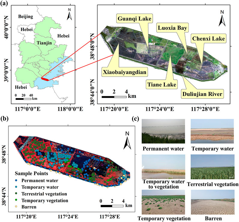
Figure 1. Location of the study area and sample points. (a) shows the geographic location of the study area, mapped with the false-color composite image of B5 (NIR), B4 (R) and B3 (G). (b) shows the spatial distribution of sample points, mapped with the true-color composite image of B4 (R), B3 (G) and B2 (b). (c) shows the field observation on 18 July 2023.

2.2 Datasets and preprocessing

2.2.1 Landsat dataset

There are all series of Landsat images on GEE, with three product types. In consideration of space, time and spectral resolution, we used Landsat-5 TM, Landsat-7 ETM+, Landsat-8 OLI and Landsat-9 OLI-2 of Level-2 types which are the surface reflectance obtained after orthophoto correction and atmospheric correction. Notably, Landsat-9 OLI-2 represents an enhanced sensor system compared to Landsat-8 OLI, featuring improved radiometric performance and enhanced signal-to-noise ratio. For each image, we selected five spectral bands: three visible bands (Blue, Green and Red), the near-infrared (NIR) band, and the short-wave infrared (SWIR) band, all with a consistent spatial resolution of 30 m. A total of 1379 images (322 Landsat-5, 654 Landsat-7, 364 Landsat-8 and 39 Landsat-9 images) covering the study area from 2000 to 2022 were collected, and the distribution of images per year is shown in Figure 2. Optical image acquisition is greatly affected by the atmosphere, and some images contain cloud noise. Therefore, we must apply cloud mask to the acquired image to remove pixels affected by clouds and cloud shadows. We used the band of “QA_PIXEL” (QA), which can detect clouds and cloud shadows of each image, to remove bad-quality observations. Finally, we generated a dataset containing all images from 2000 to 2022.

Figure 2

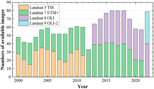
Figure 2. Numbers of Landsat images with good quality from TM/ETM+/OLI/OLI-2.

2.2.2 Meteorological dataset

In this study, we utilized the meteorological data from ERA5-Land. As a fifth-generation global climate and atmosphere reanalysis dataset, it is provided by the European Centre for Medium-Range Weather Forecasts (ECMWF), spanning from January 1950 to the present day. The spatial resolution of ERA5-Land is 9km, with an hourly temporal resolution. There are three types of datasets on GEE, including hourly, daily and monthly data. Using “ee.ImageCollection (“ECMWF/ERA5_LAND/DAILY_AGGR”), we acquired daily aggregated data, facilitating the computation of yearly data. The temperature is computed by “ee.ImageCollection.mean ()”, while the total precipitation is derived through “ee.ImageCollection.sum ()”.

2.2.3 Sample dataset

The sample points were collected on 18 July 2023. Using the Garmin eTrex 221X Outdoor Handheld GPS Navigator, we recorded the coordinates of each sample point. We recorded each type of ground objects from both sides of the road, and the areas obscured by Phragmites australis were interpreted manually aided by drone imagery. We utilized the M300 RTK equipped with a Mono×5+RGB detector, flying at an altitude of 100 m. A total of 406 sample points were collected in this study, and five classes were determined according to the actual environment: permanent water (PW), temporary water (including temporary water to vegetation) (TW, TWTV), terrestrial vegetation (TerV), temporary vegetation (TemV) and barren (B) (Figure 1b). To ensure balanced representation across all classes during training and validation, stratified random sampling method was adopted to divide all samples into two parts, with 80% allocated for training and 20% for validation. Ultimately, our dataset comprised 321 training points and 85 validation points (Table 1).

Table 1

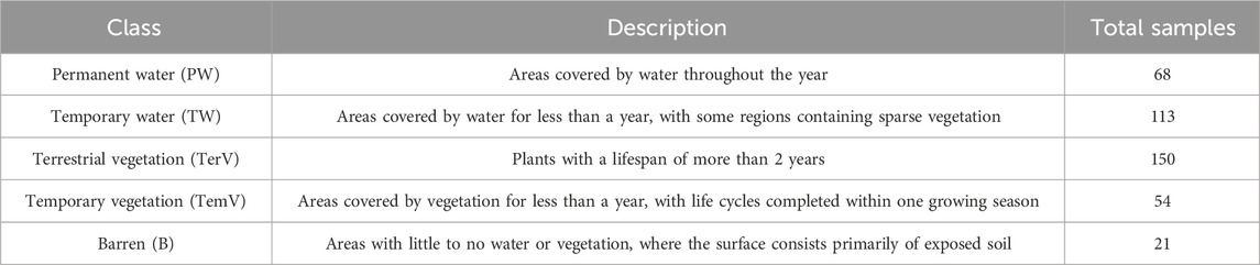
Table 1. Beidagang Wetland classification system for remote sensing.

3 Methods

In the study, GEE was utilized to analyze the dynamic changes of Beidagang Wetland during 2000–2022, including three contents. Two features, water frequency (WF) and vegetation frequency (VF), served as effective discriminators between different land types, utilizing all available images spanning the entire year. Drawing upon the prior knowledge and field observation, we delineated the ranges of WF and VF for each land type, enabling the construction of a classification rule within the Decision Tree (DT) framework. Through accuracy assessments, we obtained classification results during 2000–2022, and further analyzed these results to discern underlying driving forces shaping spatiotemporal dynamics. The overall process of the study unfolds as Figure 3.

Figure 3

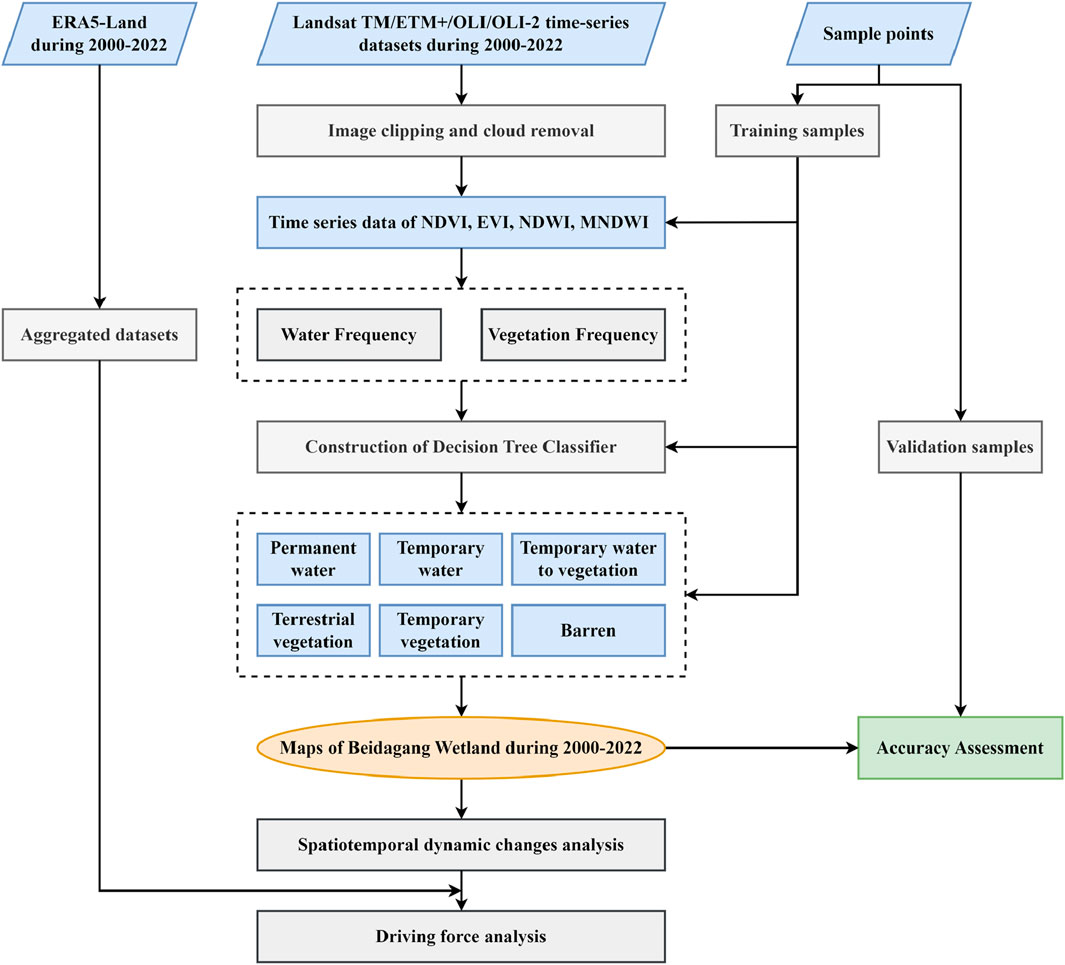
Figure 3. The framework of this study.

3.1 Identification of water pixels and vegetation pixels

Before calculating WF and VF, it is necessary to extract water and vegetation pixels. In the study, we devised methods for water and vegetation identification, employing four spectral indices: Normalized Difference Vegetation Index (NDVI), Enhanced Vegetation Index (EVI), Modified Normalized Difference Water Index (MNDWI), and Land Surface Water Index (LSWI). NDVI stands out as a robust indicator, offering insights into the spatial distribution, density, and biomass of vegetation, along with canopy background information (Tucker, 1979). EVI, an enhancement of NDVI, mitigates atmospheric interferences and exhibits heightened sensitivity in areas with high biomass (Huete et al., 2002). LSWI utilizes near-infrared and short-wave infrared bands, sensitive to moisture content of the vegetation (McFeeters, 1996). Simultaneously, we employed MNDWI, which combines green and shortwave infrared bands to enhance open water features while mitigating noise from vegetation and soil (Xu, 2006). These indices, including NDVI, NDWI, LSWI, and MNDWI, are detailed in Table 2, where ρ represents the spectral reflectance. “Blue (B)”, “Green (G)”, “Red (R)”, “NIR” and “SWIR” correspond to B1, B2, B3, B4 and B5 of Landsat-5 and Landsat-7, while for Landsat-8 and Landsat-9, they correspond to B2, B3, B4, B5, and B6.

Table 2

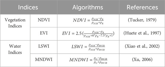
Table 2. Summary of indices.

Given the intricate wetland ecosystems and their varied structures, localized adjustments are necessary for accurately identifying water and vegetation pixels. Based on the sample points from field observation, we labeled PW points (consistently inundated throughout the year) as water pixels, and TV points (consistently vegetated throughout the year) as vegetation pixels. Additionally, we recognized the pronounced seasonal dynamics of Beidagang Wetland, particularly in its floodplain regions, which alternate between submersion and exposure. Therefore, in order to avoid bias in the final results, we utilized all available data throughout the year, to determine the threshold for identifying water and vegetation pixels.

From the preprocessed Landsat time-series data, we selected the image collection closest to the field observation time in 2022. Subsequently, time-series datasets comprising NDVI, EVI, LSWI, and MNDWI were obtained. Being overlaid with time-series datasets, each water and vegetation pixel acquired a series of index values over the course of a year. For each index, valid observations were treated as individual units, from which the three-quarters maximum, three-quarters minimum, and median values were calculated. As shown in Figure 4, “MNDWI > EVI” and “MNDWI > NDVI” serve as key indicators for identifying water pixels. Additionally, the temporal change revealed that “EVI <0.1″consistently characterizes all of water pixels throughout the year, enabling to be as a supplementary criterion. Hence, the final water pixel formula was determined as “MNDWI > EVI, MNDWI > NDVI and EVI <0.1. Furthermore, Figure 4 illustrates that EVI between 0.25 and 0.75 for vegetation pixels remains above 0 throughout the year, while NDVI values for vegetation pixels consistently exceed 0 in 2022, except for a few outliers. Therefore, we propose using these two rules for vegetation pixel identification. Additionally, apart from observations during the fifth to ninth time periods, nearly all vegetation pixel values of LSWI remained above −0.1. Consequently, we adopt “EVI ≥0, NDVI ≥0 and LSWI > −0.1″as the criteria for identifying vegetation pixels.

Figure 4

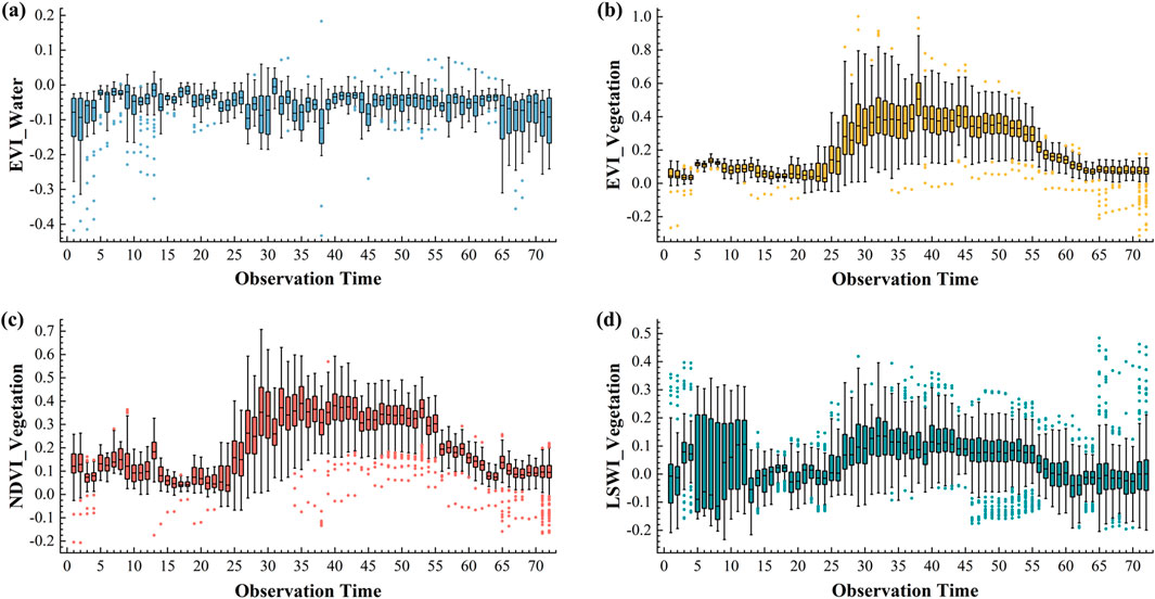
Figure 4. Temporal changes of water and vegetation pixels mapped with each index in 2022. (a) EVI of water pixels. (b) EVI of vegetation pixels. (c) NDVI of vegetation pixels. (d) LSWI of vegetation pixels.

3.2 Algorithm to identify water frequency and vegetation frequency

Due to the scarcity of good observations limited by cloud mask and the seasonal dynamics of wetland vegetation, one image or one composite image cannot fully capture the temporal changes of wetlands. In order to reduce the impact of bad-quality observations and phenological dynamics, we supposed to use frequency-based method from Landsat time-series images to characterize the differences between different land cover types. Water pixels were firstly detected using Equation 1, and then water frequency (WF) could be acquired by Equation 2.

$\sum Water=\left\{\begin{array}{l}1EVI<0.1\cap MNDWI>EVI\cap MNDWI>NDVI\\ 0Othervalues\end{array}\right.(1)$

$WF=\frac{\sum Water}{\sum Good}(2)$

Where “WF” is the frequency of water pixel occurrences within a civil year (CY), “ΣWater” represents the number of water pixels, and “ΣGood” denotes the total number of pixels with good-quality observations. In Equation 1, the criterion (MNDWI > EVI or MNDWI > NDVI) and EVI <0.1″serves as the threshold for identifying water pixels. When this criterion is met, the current pixel is classified as a water pixel, yielding a Boolean value of 1; otherwise, it returns a Boolean value of 0 for a non-water pixel. By counting the occurrences of pixels marked as 1 within a civil year, WF can be eventually obtained by Equation 2. Notably, WF’s value range from 0 to 1, with higher values indicating prolonged inundation periods throughout the year, thereby suggesting a closer resemblance to PW in terms of land cover type.

We utilized Equation 3 and Equation 4 to identify vegetation pixels and calculate vegetation frequency (VF). Pixels meeting the criterion of “(EVI ≥0 and NDVI ≥0) and LSWI > −0.1” were classified as vegetation pixels and assigned a Boolean value of 1; those failing to meet the criteria returned a Boolean value of 0 (Equation 3). Similarly, higher VF values correspond to prolonged presence of vegetation throughout the year, indicating a closer resemblance to TV.

$\sum Vegetation=\left\{\begin{array}{l}1EVI\ge 0\cap NDVI\ge 0\cap LSWI>-0.1\\ 0Othervalues\end{array}\right.(3)$

$VF=\frac{\sum Vegetation}{\sum Good}(4)$

3.3 Construction of the classification rule

Each pixel has their own WF and VF within a year, and need to be expressed in a certain way. Here, we employed the DT model to formulate a classification rule based on WF and VF. DT, an effective inductive machine learning technique, presents a hierarchical flowchart structure from root node to branch leaves, offering interpretability to a certain extent (F et al., 2016; Mueller et al., 2016). The key to constructing DT is the determination of splitting attributes (order) and splitting criteria (threshold). We collected WF and VF for all types of sample points in 2022, yielding a quantity distribution map (Figure 4). By comparing the values of WF and VF and delimiting specific ranges, we classified distinct classes within the study area.

In selecting splitting attributes, we used comparative relations between WF and VF as the root node for constructing the DT classifier. Initially, we divided land cover types into two categories: those with higher WF and those with lower WF. The former included 2 types, PW and TW. From statistical analyses (Figure 4), we established “WF-VF = 0.6″as the segmentation threshold, reflecting the most significant difference for TW delineation. For the latter, we delineated other land cover types using different criteria. Employing “WF < 0.1 and VF < 0.2,” we identified B.

Combining field observation and existing knowledge, we found Suaeda glauca and Suaeda salsa (S. glauca and S. salsa) is the dominant community in TemV. As an annual vegetation with a growing season not exceeding 6 months, we classified TemV with “VF < 0.6”, while the others belonging to TV. Additionally, we recognized a distinct land cover type, which is TW, displaying dual characteristics (Figure 5). Some points showed slightly higher WF than VF, resembling PW in spatial distribution, while others demonstrated the opposite trend, closer to TV. Therefore, we classified them separately as “WF > VF” (Figure 5b1 and “WF ≤ VF” (Figure 5b2). Considering the temporal characteristics of the growing season, we ultimately utilized “0.1≤WF ≤ 0.4 and 0.2≤VF < 0.6″to identify TemV, with the other type labelled as TWTV. The specific flow of DT is illustrated in Figure 6.

Figure 5

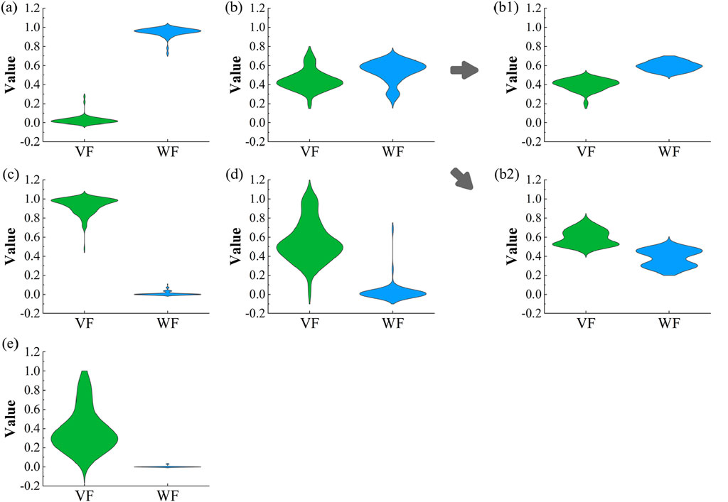
Figure 5. Map of quantity distribution in WF and VF for each type of sample points. (a) Permanent water. (b) Temporary water. (b1) Temporary water (WF > VF). (b2) Temporary water to vegetation (WF ≤ VF) (c) Terrestrial vegetation. (d) Temporary vegetation. (e) Barren.

Figure 6

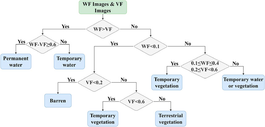
Figure 6. Construction of DT classifier based on WF and VF.

3.4 Method of validation

The accuracy of classification results is evaluated by calculating the confusion matrix based on validation samples. The confusion matrix, also known as the error matrix, is the most basic, intuitive, and simplest method to calculate the accuracy of a classification model (Svoboda et al., 2022). In image accuracy evaluation, confusion matrix is mainly used to compare classification results with actual measured points (Duro et al., 2012). More advanced classification indicators can be obtained from the confusion matrix. In the study, we selected Overall Accuracy (OA), Kappa coefficient, Producer’s Accuracy (PA) and User’s Accuracy (UA) for accuracy assessment. OA refers to the proportion of correctly classified pixels relative to the total number of pixels. The Kappa coefficient is calculated using Equation 5.

$\mathit{K}\mathit{a}\mathit{p}\mathit{p}\mathit{a}=\frac{{\mathit{P}}_{\mathbf{0}}-{\mathit{P}}_{\mathit{e}}}{\mathbf{1}-{\mathit{P}}_{\mathit{e}}}(5)$

Among them, “P0” is for OA, “Pe” is calculated as the sum of the products of the actual and predicted quantities for all categories, divided by the square of the sum of the matrix elements. The Kappa coefficient ranges from −1 to 1, usually greater than 0. The higher Kappa coefficient, the better the classification effect. What’s more, the producer’s Accuracy is the probability that the real reference data of a certain type is correctly classified (Dai et al., 2021). The user’s accuracy is calculated by dividing the reference data of a certain type by the real collected points (Dai et al., 2021).

4 Results

4.1 Accuracy assessment of classification results

Since the field observation in 2023, we have utilized the classification result in 2022, closest to the measurement period, for accuracy assessment and constructing the confusion matrix (Table 3). The OA derived from this matrix is 89.41%, with the Kappa coefficient of 0.85, indicating a high degree of accuracy. Upon the User’s Accuracy and the Producer’s Accuracy derived from the confusion matrix, we observed notable misclassifications within contiguous land cover types, particularly among TW, TV, and TemV. TemV, primarily comprising S. glauca and S. salsa, occupying dry or exposed river floodplains, is more likely to be misidentified as TW. This misidentification often occurs due to the floodplains’ intermittent submergence following sudden precipitation or ecological replenishment, resulting in a scarcity of TemV. Consequently, the spectral characteristics captured in Landsat images may exhibit similarities between TW and TemV, leading to comparable values in WF and subsequent misclassifications.

Table 3

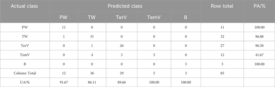
Table 3. Accuracy assessment of classification result in 2022 using the confusion matrix.

Furthermore, we also conducted an accuracy assessment of historical results from 2000, 2004, 2010, 2016, and 2020. For validation sample preparation, we employed a sample migration approach based on 2023 field observations. Spectral Angle Distance (SAD) and Euclidean Distance (ED) were used to assess spectral similarity across temporal intervals, yielding temporally consistent validation points for each target year (Huang et al., 2020). Given the limited number of migrated samples meeting stability criteria, we supplemented the validation dataset through the visual interpretation of high-resolution Google Earth (GE) images to ensure adequate representation across all land cover types. Classification accuracy was assessed using the collected validation samples for each year, with results presented in Table 4. The consistently high accuracy across all target years demonstrates that the DT-based classification method using WF and VF is reliable and suitable for long-term wetland monitoring applications.

Table 4

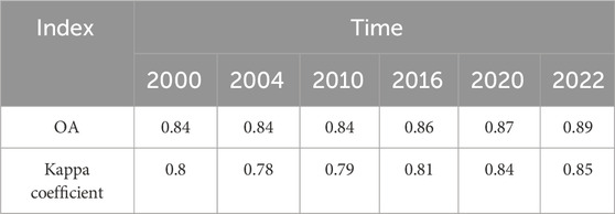
Table 4. Accuracy assessment in 2000, 2004, 2010, 2016, 2020, and 2022.

4.2 Spatial variation in Beidagang Wetland during 2000-2022

Using the DT model based on WF and VF, we generated the spatial distribution of each land cover type in Beidagang Wetland from 2000 to 2022 (Figure 7). To mitigate the impact of strip noise on classification results, data from 2005, 2008, 2011, and 2012 were excluded, resulting in a total of 19 retained classification maps from other years. The distinct spatial distribution patterns among different land cover types, each adhering to specific rules, are illustrated in Figure 7. TW and TWTV are frequently observed at the peripheries of PW. Within expansive floodplain regions, TWTV encircles TW, creating a transitional zone with TV. TemV typically thrives within the transition zone, bridging the gap between TWTV and TV. Characteristically, these patches exhibit elongated and narrow shapes, with small and highly fragmented areas.

Figure 7

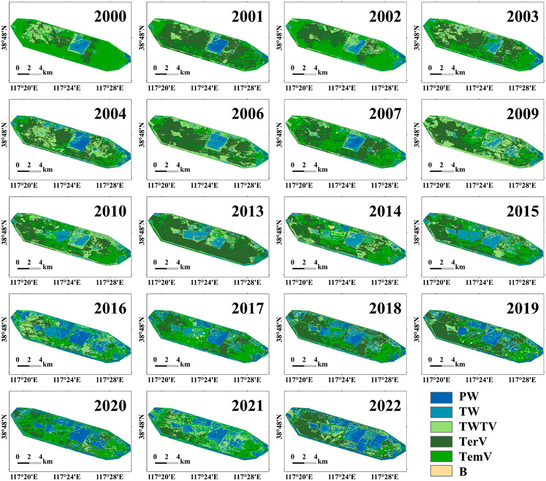
Figure 7. Spatial distribution of six land cover types in Beidagang Wetland during 2000–2022.

To present the details of land cover changes in Beidagang Wetland, the type conversion was employed in Figure 8. The dynamics of different land cover types within Beidagang Wetland exhibit a relatively intricate pattern of changes, primarily observed in four key regions: Xiaobaiyangdian, Guanqi Lake, Tiane Lake, and Chenxi Lake (Figure 8a). Xiaobaiyangdian, situated west of the study area, transitioned from extensive TemV to TV, remaining predominantly vegetated from 2000 to 2022 (Figure 8b). Conversely, a significant transformation occurred in Chenxi Lake. Previously characterized by TemV in 2000, it has evolved into PW by 2022, marking considerable interannual variations in land cover types over the past 2 decades.

Figure 8

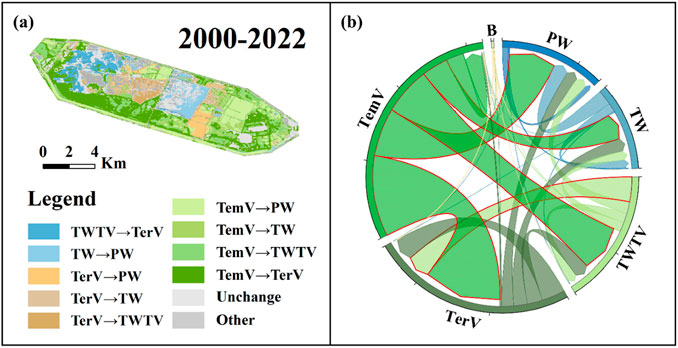
Figure 8. Type conversion during 2000–2022. (a) Shows the spatial conversion of major land cover types. (b) Shows the conversion ratio of each type and the most varied type highlighted in red.

Guanqi Lake, located centrally in the study area, depict the most pronounced interannual changes in land cover types. Since 2000, It has witnessed fluctuating changes of TV, TemV, PW and TW, with concurrent existence of TW and TWTV. Furthermore, Tiane Lake, in the middle of the study area, has remained water-covered since 2000, albeit in different forms. Notably, the expanse of PW has expanded, primarily along the eastern shoreline, while TW persisted near the western coast. Additionally, the centralized place of bird has facilitated the growth of aquatic vegetation in the lake’s central region. These areas have undergone substantial changes over the past 2 decades, with significant alterations in land cover types.

4.3 Temporal changes in Beidagang Wetland during 2000-2022

To observe the temporal changes of Beidagang Wetland, we initially conducted a Spearman correlation analysis to identify areas where NDVI, WF, and VF significantly correlated with time (p < 0.05). Subsequently, we calculated the gradient of these features over time (Figure 9a). The analysis identified three regions exhibiting notable correlations with time: Luoxia Bay, Duliujian River, Guanqi Lake and its northern area. However, differences emerged between features within these significantly correlated regions. Specifically, in Xiaobaiyangdian, an area dominated by TV, NDVI exhibited minimal gradient change, indicating relatively stable TV coverage, while VF showed a low correlation with time. This relative stability in VF, coupled with a slight increase in NDVI, suggests that TV coverage has remained largely unchanged, albeit with slight growth improvements compared to 2000.

Figure 9

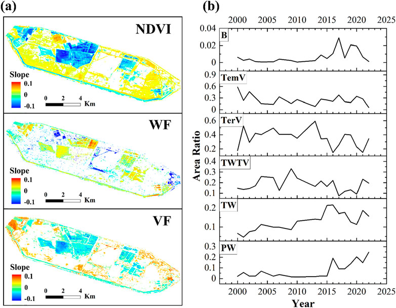
Figure 9. (a) Temporal changes of NDVI, WF and VF in Beidagang Wetland during 2000–2022. (b) The area ratio’s change of six land cover types during 2000–2022.

We also compared regions with higher gradients. The gradient changes of NDVI and VF revealed a significant reduction in Guanqi Lake over the past 20 years, whereas WF changes varied across these regions. Notably, there was a significant increase of WF in the northern areas, while within Guanqi Lake, WF exhibited differences. Specifically, WF in the west of Guanqi Lake showed a slight increase over time, while in the east, there were interannual fluctuations in WF, lacking a clear change pattern. The decline of vegetation in Guanqi Lake was accompanied by an increase of water, as evidenced by the classification map, indicating a gradual transformation to a water-dominated area in recent years.

Furthermore, we analyzed the interannual changes in the area proportion of each land cover type in Beidagang Wetland. Figure 9b reveals that the area of PW remained basically stable before 2015, with the proportion consistently below 0.1. However, substantial changes occurred after 2015, leading to an overall increasing trend. By 2022, the proportion of PW had exceeded 0.2. The area occupied by TW generally expanded since 2000, despite slight declines in some years. From 2000 to 2014, the proportion of TW increased gradually, but after 2015, significant fluctuations were observed. TW experienced a slight decrease during 2016–2020, followed by a little increase in 2021, maintaining an overall ratio between 0.1 and 0.2. The change of TW after 2016 corresponded to those of PW, suggesting a spatial redistribution between these two types.

Among various vegetation types, the proportion of transient vegetation area fluctuated slightly within the range of 0–0.3, indicating a gradual decline over time. The most significant interannual fluctuations and the absence of clear change patterns were observed in TWTV and TV. The proportion of TWTV remained low during 2016–2020, fluctuating around 0.2 in subsequent years. Although TV is the dominant community in Beidagang Wetland, its overall proportion has decreased since 2014, showing interannual instability. B has consistently constituted the smallest land cover type in Beidagang Wetland, exhibiting little change compared to water and vegetation.

In summary, the interannual changes in Beidagang Wetland can be divided into two distinct periods: from 2000 to 2014 and from 2015 to 2022. During the first period (2000–2014), the wetland was characterized by vegetation dominance and stable PW areas, with slight increases in TW. In contrast, the second period (2015–2022), saw a notable overall downward trend in vegetation types alongside an increase in PW, while TW exhibited minor fluctuations.

4.4 Long-term changes of WF and VF in Beidagang Wetland during 2000-2022

To more intuitively represent the spatial variation characteristics of Beidagang Wetland, we divided WF into four levels: 0–0.1 (poor), 0.1–0.4 (adequate), 0.4–0.9 (good), 0.9–1 (excellent) (More detailed results are provided in Supplementary Figure 1). As shown in Figure 10a, WF pixels between “0–0.1” are mainly distributed in the southwest and southeast of the study area, where the dominant land cover types are TV and TemV. Pixels in the “0.1–0.4” are unevenly distributed across years, with sparse and fragmented spatial patterns, typically found near areas with higher WF values. In contrast, the spatial distribution of pixels in the “0.4–0.9” and “0.9–1” is more stable, primarily concentrated in the central part of the study area, especially around Tiane Lake and Guanqi Lake. However, the distribution varies annually, with type shifts occurring mainly between “0.4–0.9” and “0.9–1”.

Figure 10

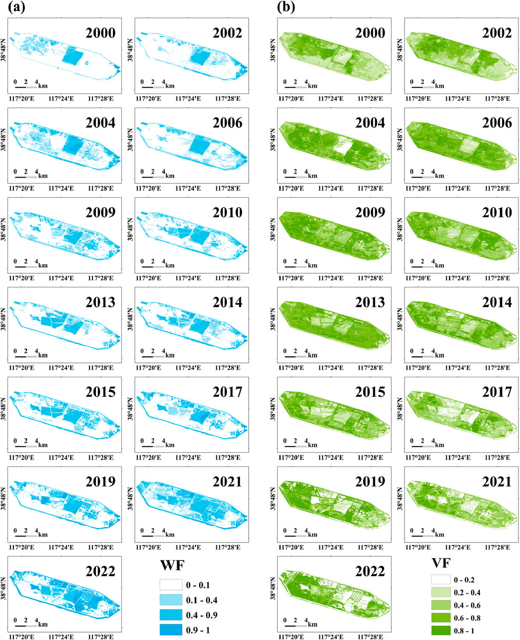
Figure 10. Spatial distribution of WF (a) and VF (b) in Beidagang Wetland during 2000–2022.

Similarly, VF was divided into five levels: 0–0.2 (poor), 0.2–0.4 (average), 0.4–0.6 (adequate), 0.6–0.8 (good), 0.8–1 (excellent). The classification results for major years are shown in Figure 10b (More detailed results are provided in Supplementary Figure 2). Overall, the vegetation distribution has gradually shifted from the center to the southwest and northwest of the study area, while Xiaobaiyangdian has consistently remained the main area of vegetation distribution. From Figure 10b, the areas of high values are gradually decreasing, with a trend toward spatial fragmentation. Precipitation fluctuations significantly impact this interannual variation, leading to a degree of mutual transformation between areas of excellent growth (0.8–1) and good growth (0.6–0.8).

There is a clear correspondence between WF and VF. Areas with higher WF tend to correspond with lower VF, consistent with the distribution of wetland water. In Xiaobaiyangdian and its surroundings, VF remains high, typically associated with WF values in the “0–0.1”. Areas with adequate (0.1–0.4) or good (0.4–0.9) levels of WF and adequate (0.4–0.6) levels of VF are mainly located near Guanqi Lake.

5 Discussion

5.1 Driving factors

The spatial and temporal dynamics of Beidagang Wetland are shaped by a combination of natural and human influences. Natural factors, such as variations in temperature and precipitation, play a significant role in these changes. Additionally, human activities, including the enhancement of legal frameworks and the implementation of wetland restoration initiative, also exert a substantial impact on the wetland ecosystem.

5.1.1 Natural factors

To test whether the fluctuations in temperature and precipitation influenced the dynamics of land cover types within Beidagang Wetland, we collected data on annual temperature, annual total precipitation in Beidagang Wetland during 2000–2022, alongside calculating WF of Duliujian River during 2000–2020. As shown in Figure 11, the temperature fluctuated between years, showing an overall increasing trend. Temperature increases can extend growing seasons and enhance the productivity of salt marsh vegetation, which is also consistent with changes of NDVI (Figure 9a). Additionally, temperature variations can indirectly induce changes of hydrological parameters, affecting the redistribution of land cover types (Zhang C. et al., 2021).

Figure 11

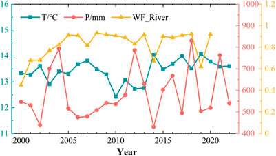
Figure 11. Temperature and precipitation of Beidagang Wetland during 2000–2022, and WF of Duliujian River (WF_River) during 2000–2020.

Precipitation serves as a vital water source for wetlands, and alterations in precipitation patterns can lead to substantial modifications in wetland hydrology and aquatic ecosystems. Figure 11 illustrates the significant year-to-year fluctuations in precipitation, whether sharp increases or decreases, resulting in notable interannual changes in land cover types across Beidagang Wetland. Increased precipitation, contracts the habitat of TemV, causing a shift in land cover towards floodplains. Conversely, decreased precipitation reduces the extent of TW, enlarging the narrow transition zone between water and vegetation.

Furthermore, water replenishment from Duliujian River also plays a pivotal role in shaping the spatiotemporal dynamics of Beidagang Wetland. Figure 11 reveals a gradual increasing trend of WF from 2000 to 2020, consistent with changes of wetland water, albeit with minor fluctuations in some years. Prior to 2005, WF of Duliujian River was lower than 0.9, essentially devoid of flow, and unable to provide water replenishment for Beidagang Wetland. Once WF stabilized at about 0.9, Duliujian River was capable of supporting additional water resources for Beidagang Wetland. However, rivers are not the primary source of water replenishment, therefore, temporary fluctuations exert little impact on the distribution of land cover types.

5.1.2 Human factors

Beidagang Wetland has experienced severe degradation over an extended period due to irrational utilization and destruction. In response, the Chinese government has implemented various efforts aimed at restoring the wetland ecosystem (Figure 12). Before 2008, the efforts focused on its conservation, scientific research, tourism and public awareness, therefore, the overall recovery progressed at a relatively slow rate. With the range adjustment and functional zoning (core, buffer, experimental areas) of Beidagang Wetland in 2008, the distribution of each land cover type gradually became more standardized. The hydrological resources in Beidagang Wetland are primarily concentrated in Tiane Lake, Luoxia Bay and Guanqi Lake, with additional water bodies radiating outward from three major areas. TerV occurs in fragmented patches adjacent to the water areas, with the highest density cencentrated occurring in the Xiaobaiyangdian (Figures 7, 10). These initiatives corresponded to the interannual changes of TW and TerV (Figure 9b), exhibiting a stable but slowly increasing trend over time.

Figure 12

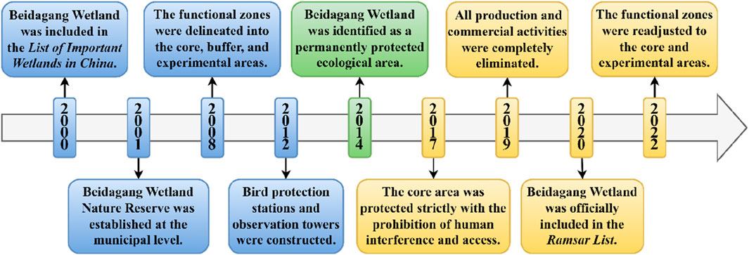
Figure 12. Changes of policies in Beidagang Wetland from 2000 to 2022.

Since 2014, ecological compensation for Beidagang Wetland has intensified. Measures including ecological water replenishment and water environment management have resulted in a noticeable expansion of wetland water (Sun and Sun, 2021). Guanqi Lake, situated within the core area, has undergone transitions from TerV to TW and TWTV. The negative correlations between NDVI, VF and time, coupled with the non-significant relationship between WF and time (Figure 9a), proved the dominant role of human factors in driving wetland transformations. Furthermore, systematic functional zoning has been implemented, with all production and living activities being phased out from the core area (Chai et al., 2020). Luoxia Bay, formerly utilized for aquaculture, has demonstrated annual increases in WF since 2017 (Figure 10a), indicating successful restoration to suitable bird habitat. Concurrently, vegetation restoration efforts utilizing native species such as Phragmites and Suaeda have been implemented, while invasive Spartina populations have been systematically controlled (Sun and Sun, 2021). These restoration measures have significantly improved the wetland’s ecological environment, abundance and diversity of migratory birds, and establishing favorable conditions for regional sustainable development.

5.2 Uncertainties and limitations

The accuracy of classification results mostly depends on the accuracy of sample points. Since there is no existing dataset to support it, only 1 year of actual sample points can be relied on to determine the classification standard, which may lead to a certain degree of error. Especially for the land cover types with large spatiotemporal variations, such as TemV, the sample points of only 1 year still cannot contain all dynamic change information. Additionally, our analysis of the confusion matrix reveals clusters of misclassifications within contiguous land cover types. Despite deliberate efforts to position sample points away from transitional zones, the intersecting numerical distributions of WF between adjacent classes pose challenges for direct classification using a binary model. While these misclassified pixels are relatively sparse and minimally affect OA, they do influence the evaluation of Kappa coefficient.

5.3 Applicability and future applications

The DT classifier based on WF and VF demonstrates potentially broad applicability for large-scale wetland monitoring. Its superior interpretability enables threshold optimization tailored to regional characteristics while facilitating the selection of classification features based on the physiological and ecological properties of vegetation. Moreover, the computational efficiency makes this method well-suited for large-scale applications where traditional machine learning approaches may encounter resource constraints (Zhang et al., 2023; Wang et al., 2020a; Wang et al., 2020b; Liu et al., 2023; Zhao et al., 2024; Zhang et al., 2020; Chen et al., 2017). Currently, deep learning and machine learning have been gradually applied to wetland classification (Chen et al., 2020; Hosseiny et al., 2022; Zhang et al., 2022; Aslam et al., 2024a; Aslam et al., 2024b; Berhane et al., 2018). Future developments will focus on synthesizing advanced computational methods with transparent, interpretable frameworks to enhance both classification accuracy and ecological understanding. As satellite data archives continue expanding, this approach can provide consistent and interpretable results for multi-decadal wetland classification across diverse geographical regions.

6 Conclusion

This study utilized Landsat-5/7/8/9 time-series images and GEE to develop a DT-based classification method for monitoring spatiotemporal dynamics of Beidagang Wetland from 2000 to 2022. The approach employed optimized thresholds of WF and VF to characterize land cover types and revealed the driving factors underlying wetland changes. The flowing conclusions drawn from our study revealed that:

(1) The DT-based classification method achieved the OA of 0.89 with the Kappa coefficient of 0.85, demonstrating the reliability of WF and VF for wetland classification.

(2) During 2000–2022, Beidagang Wetland exhibited substantial changes characterized by increasing water areas and declining vegetation communities, while other land cover types remained stable and limited spatial coverage. The areas where NDVI, WF, and VF showed significant temporal correlations were primarily located in Luoxia Bay, Duliujian River, and Guanqi Lake. In contrast, Tiane Lake displayed non-significant correlations among these three variables over time. Guanqi Lake demonstrated the largest vegetation reduction gradient; however, in the eastern areas dominated by TW and TWTV, the correlation between WF was not evident.

(3) Based on interannual variability and policy adjustments, two distinct periods were identified. From 2000 to 2014, Beidagang Wetland was characterized by TerV dominance, with PW occupying less than 10% of the total area and TW showing a gradual increase. From 2015 to 2022, PW expanded to exceed 20%, accompanied by declining TerV coverage and fluctuating TWTV at approximately 20%. TWTV and TerV presented the greatest variability over the past 2 decades, with potential spatial transitions occurring between TW and PW.

(4) Land cover types exhibited a radial distribution pattern centered on Tiane Lake, extending toward peripheral areas including Guanqi Lake and Luoxia Bay, with the Duliujian River serving as a north-south boundary. PW and TerV concentrated primarily in the Tiane Lake and Xiaobaiyangdian, while TW and TWTV occupied intermediate transitional zones.

(5) Complex type conversions occurred predominantly in four critical areas: Guanqi Lake, Tiane Lake, Xiaobaiyangdian, and eastern Luoxia Bay. Guanqi Lake, located in the center of Beidagang Wetland, exhibited the most significant change, transitioning from TerV to TW.

(6) Wetland dynamics resulted from the complex interaction of natural and anthropogenic factors. Climate variables, including rising temperatures and precipitation deficits, contributed to wetland water volume reduction and extension of transition zones. Conservation management interventions, including functional zoning, comprehensive withdrawal of human activities, and ecological restoration initiatives, facilitated wetland water area expansion, enhanced avifaunal diversity, and improved overall ecosystem integrity.

The results indicate that DT-based classification method using WF and VF effectively captures long-term wetland dynamics through annual remote sensing imagery. Compared to traditional single-date approaches and machine learning algorithms, this method offers superior interpretability, computational efficiency, and cost-effectiveness while maintaining high classification accuracy. These findings provide valuable insights for wetland ecosystem monitoring and support evidence-based conservation management at large spatiotemporal scales.

Data availability statement

The raw data supporting the conclusions of this article will be made available by the authors, without undue reservation.

Author contributions

XZ: Data curation, Formal Analysis, Investigation, Methodology, Validation, Visualization, Writing – original draft, Writing – review and editing. TW: Conceptualization, Data curation, Funding acquisition, Investigation, Methodology, Project administration, Resources, Supervision, Writing – review and editing. XH: Conceptualization, Data curation, Funding acquisition, Investigation, Methodology, Project administration, Resources, Supervision, Writing – review and editing.

Funding

The author(s) declare that financial support was received for the research and/or publication of this article. The research was supported by the Special Foundation for National Science and Technology Basic Research Program of China (Grant No. 2021FY101003) and the National Natural Science Foundation of China (Grant No. 4230010663).

Conflict of interest

The authors declare that the research was conducted in the absence of any commercial or financial relationships that could be construed as a potential conflict of interest.

Generative AI statement

The author(s) declare that no Generative AI was used in the creation of this manuscript.

Publisher’s note

All claims expressed in this article are solely those of the authors and do not necessarily represent those of their affiliated organizations, or those of the publisher, the editors and the reviewers. Any product that may be evaluated in this article, or claim that may be made by its manufacturer, is not guaranteed or endorsed by the publisher.

Supplementary material

The Supplementary Material for this article can be found online at: https://www.frontiersin.org/articles/10.3389/frsen.2025.1569617/full#supplementary-material

References

Amani, M., Mahdavi, S., Afshar, M., Brisco, B., Huang, W., Mohammad Javad Mirzadeh, S., et al. (2019). Canadian wetland inventory using google Earth engine: the first map and preliminary results. Remote Sens. 11 (7), 842. doi:10.3390/rs11070842

CrossRef Full Text | Google Scholar

Anderson, C. J., Heins, D., Pelletier, K. C., and Knight, J. F. (2023). Using voting-based ensemble classifiers to map invasive Phragmites australis. Remote Sens. 15 (14), 3511. doi:10.3390/rs15143511

CrossRef Full Text | Google Scholar

Aslam, R. W., Shu, H., and Yaseen, A. (2023). Monitoring the population change and urban growth of four major Pakistan cities through spatial analysis of open source data. Ann. GIS 29 (3), 355–367. doi:10.1080/19475683.2023.2166989

CrossRef Full Text | Google Scholar

Aslam, R. W., Naz, I., Shu, H., Yan, J., Quddoos, A., Tariq, A., et al. (2024a). Multi-temporal image analysis of wetland dynamics using machine learning algorithms. J. Environ. Manag. 371, 123123. doi:10.1016/j.jenvman.2024.123123

PubMed Abstract | CrossRef Full Text | Google Scholar

Aslam, R. W., Shu, H., Naz, I., Quddoos, A., Yaseen, A., Gulshad, K., et al. (2024b). Machine learning-based wetland vulnerability assessment in the Sindh province ramsar site using remote sensing data. Remote Sens. 16 (5), 928. doi:10.3390/rs16050928

CrossRef Full Text | Google Scholar

Aslam, R. W., Shu, H., Tariq, A., Naz, I., Ahmad, M. N., Quddoos, A., et al. (2024c). Monitoring landuse change in uchhali and khabeki wetland Lakes, Pakistan using remote sensing data. Gondwana Res. 129, 252–267. doi:10.1016/j.gr.2023.12.015

CrossRef Full Text | Google Scholar

Belgiu, M., and Drăguţ, L. (2016). Random forest in remote sensing: a review of applications and future directions. ISPRS J. Photogrammetry Remote Sens. 114, 24–31. doi:10.1016/j.isprsjprs.2016.01.011

CrossRef Full Text | Google Scholar

Berhane, T. M., Lane, C. R., Wu, Q., Autrey, B. C., Anenkhonov, O. A., Chepinoga, V. V., et al. (2018). Decision-tree, Rule-Based, and random Forest classification of high-resolution multispectral imagery for wetland mapping and inventory. Remote Sens. (Basel). 10 (4), 580. doi:10.3390/rs10040580

PubMed Abstract | CrossRef Full Text | Google Scholar

Chai, Z., Lei, W., Mo, X., Que, P., Shang, C., Yang, J., et al. (2020). Bird diversity of Beidagang wetland nature reserve in Tianjin city. Wetl. Sci. 18, 667–678. doi:10.13248/j.cnki.wetlandsci.2020.06.005

CrossRef Full Text | Google Scholar

Chen, B., Xiao, X., Li, X., Pan, L., Doughty, R., Ma, J., et al. (2017). A mangrove forest map of China in 2015: analysis of time series Landsat 7/8 and Sentinel-1A imagery in Google Earth Engine cloud computing platform. ISPRS J. Photogrammetry Remote Sens. 131, 104–120. doi:10.1016/j.isprsjprs.2017.07.011

CrossRef Full Text | Google Scholar

Chen, M., Ke, Y., Bai, J., Li, P., Lyu, M., Gong, Z., et al. (2020). Monitoring early stage invasion of exotic Spartina alterniflora using deep-learning super-resolution techniques based on multisource high-resolution satellite imagery: a case study in the Yellow River Delta, China. Int. J. Appl. Earth Observation Geoinformation 92, 102180. doi:10.1016/j.jag.2020.102180

CrossRef Full Text | Google Scholar

Dai, Y., Feng, L., Hou, X., and Tang, J. (2021). An automatic classification algorithm for submerged aquatic vegetation in shallow lakes using Landsat imagery. Remote Sens. Environ. 260, 112459. doi:10.1016/j.rse.2021.112459

CrossRef Full Text | Google Scholar

de la Fuente, A., Meruane, C., and Suarez, F. (2021). Long-term spatiotemporal variability in high Andean wetlands in northern Chile. Sci. Total Environ. 756, 143830. doi:10.1016/j.scitotenv.2020.143830

PubMed Abstract | CrossRef Full Text | Google Scholar

DeVries, B., Huang, C., Lang, M., Jones, J., Huang, W., Creed, I., et al. (2017). Automated quantification of surface water inundation in wetlands using optical satellite imagery. Remote Sens. 9 (8), 807. doi:10.3390/rs9080807

CrossRef Full Text | Google Scholar

Duro, D. C., Franklin, S. E., and Dubé, M. G. (2012). A comparison of pixel-based and object-based image analysis with selected machine learning algorithms for the classification of agricultural landscapes using SPOT-5 HRG imagery. Remote Sens. Environ. 118, 259–272. doi:10.1016/j.rse.2011.11.020

CrossRef Full Text | Google Scholar

Erwin, K. L. (2008). Wetlands and global climate change: the role of wetland restoration in a changing world. Wetl. Ecol. Manag. 17 (1), 71–84. doi:10.1007/s11273-008-9119-1

CrossRef Full Text | Google Scholar

Fisher, A., Flood, N., and Danaher, T. (2016). Comparing Landsat water index methods for automated water classification in eastern Australia. Remote Sens. Environ. 175, 167–182. doi:10.1016/j.rse.2015.12.055

CrossRef Full Text | Google Scholar

Feng, S., Li, W., Xu, J., Liang, T., Ma, X., Wang, W., et al. (2022a). Land Use/Land cover mapping based on GEE for the monitoring of changes in ecosystem types in the upper yellow River Basin over the Tibetan Plateau. Remote Sens. 14 (21), 5361. doi:10.3390/rs14215361

CrossRef Full Text | Google Scholar

Feng, K., Mao, D., Qiu, Z., Zhao, Y., and Wang, Z. (2022b). Can time-series Sentinel images be used to properly identify wetland plant communities? GIScience and Remote Sens. 59 (1), 2202–2216. doi:10.1080/15481603.2022.2156064

CrossRef Full Text | Google Scholar

Gell, P. A., Finlayson, C. M., and Davidson, N. C. (2023). “An introduction to the Ramsar Convention on Wetlands,” in Ramsar wetlands. Elsevier, 1–36.

CrossRef Full Text | Google Scholar

Gong, P., Wang, J., and Huang, H. (2024). Stable classification with limited samples in global land cover mapping: theory and experiments. Sci. Bull. (Beijing). 69 (12), 1862–1865. doi:10.1016/j.scib.2024.03.040

PubMed Abstract | CrossRef Full Text | Google Scholar

Guo, L., Zhao, S., Gao, J., Zhang, H., Zou, Y., and Xiao, X. (2022). A novel workflow for crop type mapping with a time series of synthetic aperture radar and optical images in the Google Earth engine. Remote Sens. 14 (21), 5458. doi:10.3390/rs14215458

CrossRef Full Text | Google Scholar

Han, X., Feng, L., Hu, C., and Chen, X. (2018). Wetland changes of China's largest freshwater lake and their linkage with the Three Gorges Dam. Remote Sens. Environ. 204, 799–811. doi:10.1016/j.rse.2017.09.023

CrossRef Full Text | Google Scholar

Han, M., Pan, B., Liu, Y. B., Yu, H. Z., and Liu, Y. R. (2019). Wetland biomass inversion and space differentiation: a case study of the Yellow River Delta Nature Reserve. PLoS One 14 (2), e0210774. doi:10.1371/journal.pone.0210774

PubMed Abstract | CrossRef Full Text | Google Scholar

Hao, Z., Haseeb, M., Xiangtian, Z., Tahir, Z., Mahmood, S. A., Tariq, A., et al. (2025). Multitemporal analysis of urbanization-driven slope and ecological impact using machine-learning and remote sensing techniques. IEEE J. Sel. Top. Appl. Earth Observations Remote Sens. 18, 1876–1895. doi:10.1109/jstars.2024.3509133

CrossRef Full Text | Google Scholar

Hosseiny, B., Mahdianpari, M., Brisco, B., Mohammadimanesh, F., and Salehi, B. (2022). WetNet: a spatial–temporal ensemble deep learning model for wetland classification using Sentinel-1 and Sentinel-2. IEEE Trans. Geoscience Remote Sens. 60, 1–14. doi:10.1109/tgrs.2021.3113856

CrossRef Full Text | Google Scholar

Hu, L., Xu, N., Liang, J., Li, Z., Chen, L., and Zhao, F. (2020). Advancing the mapping of mangrove forests at national-scale using Sentinel-1 and Sentinel-2 time-series data with Google Earth engine: a case Study in China. Remote Sens. 12 (19), 3120. doi:10.3390/rs12193120

CrossRef Full Text | Google Scholar

Huang, H., Wang, J., Liu, C., Liang, L., Li, C., and Gong, P. (2020). The migration of training samples towards dynamic global land cover mapping. ISPRS J. Photogrammetry Remote Sens. 161, 27–36. doi:10.1016/j.isprsjprs.2020.01.010

CrossRef Full Text | Google Scholar

Huete, A., Didan, K., Miura, T., Rodriguez, E. P., Gao, X., and Ferreira, L. G. (2002). Overview of the radiometric and biophysical performance of the MODIS vegetation indices. Remote Sens. Environ. 83 (1-2), 195–213. doi:10.1016/s0034-4257(02)00096-2

CrossRef Full Text | Google Scholar

Jamali, A., Mahdianpari, M., Brisco, B., Granger, J., Mohammadimanesh, F., and Salehi, B. (2021). Deep Forest classifier for wetland mapping using the combination of Sentinel-1 and Sentinel-2 data. GIScience and Remote Sens. 58 (7), 1072–1089. doi:10.1080/15481603.2021.1965399

CrossRef Full Text | Google Scholar

Ju, Y., and Bohrer, G. (2022). Classification of wetland vegetation based on NDVI time series from the HLS dataset. Remote Sens. 14 (9), 2107. doi:10.3390/rs14092107

CrossRef Full Text | Google Scholar

Kazemi, G. M., Weng, Q., Hossein Haghi, V., Li, Z., Kazemi Garajeh, A., and Salmani, B. (2022). Learning-Based methods for detection and monitoring of shallow flood-affected areas: impact of shallow-flood spreading on vegetation density. Can. J. Remote Sens. 48 (4), 481–503. doi:10.1080/07038992.2022.2072277

CrossRef Full Text | Google Scholar

Keddy, P. A. (2010). Wetland ecology: principles and conservation. Cambridge, United Kingdom: Cambridge University Press.

Google Scholar

Kool, J., Lhermitte, S., Hrachowitz, M., Bregoli, F., and McClain, M. E. (2022). Seasonal inundation dynamics and water balance of the Mara Wetland, Tanzania based on multi-temporal Sentinel-2 image classification. Int. J. Appl. Earth Observation Geoinformation 109, 102766. doi:10.1016/j.jag.2022.102766

CrossRef Full Text | Google Scholar

Kuchara, V., Charan, R., Mankad, A., and Solanki, H. (2023). Wetland degradation and loss due to the expansion of anthropogenic activities. Int. Assoc. Biol. Comput. Dig. 2 (2), 41–47. doi:10.56588/iabcd.v2i2.191

CrossRef Full Text | Google Scholar

Leblanc, M., Lemoalle, J., Bader, J. C., Tweed, S., and Mofor, L. (2011). Thermal remote sensing of water under flooded vegetation: new observations of inundation patterns for the ‘Small’ Lake Chad. J. Hydrology 404 (1-2), 87–98. doi:10.1016/j.jhydrol.2011.04.023

CrossRef Full Text | Google Scholar

Liu, Y., Xiao, X., Li, J., Wang, X., Chen, B., Sun, C., et al. (2023). Tracking changes in coastal land cover in the Yellow Sea, East Asia, using Sentinel-1 and Sentinel-2 time-series images and Google Earth Engine. ISPRS J. Photogrammetry Remote Sens. 196, 429–444. doi:10.1016/j.isprsjprs.2022.12.029

CrossRef Full Text | Google Scholar

Ludwig, C., Walli, A., Schleicher, C., Weichselbaum, J., and Riffler, M. (2019). A highly automated algorithm for wetland detection using multi-temporal optical satellite data. Remote Sens. Environ. 224, 333–351. doi:10.1016/j.rse.2019.01.017

CrossRef Full Text | Google Scholar

Mahdavi, S., Salehi, B., Granger, J., Amani, M., Brisco, B., and Huang, W. (2017). Remote sensing for wetland classification: a comprehensive review. GIScience and Remote Sens. 55 (5), 623–658. doi:10.1080/15481603.2017.1419602

CrossRef Full Text | Google Scholar

Mahdianpari, M., Salehi, B., Mohammadimanesh, F., and Motagh, M. (2017). Random forest wetland classification using ALOS-2 L-band, RADARSAT-2 C-band, and TerraSAR-X imagery. ISPRS J. Photogrammetry Remote Sens. 130, 13–31. doi:10.1016/j.isprsjprs.2017.05.010

CrossRef Full Text | Google Scholar

Mao, D., Wang, Z., Du, B., Li, L., Tian, Y., Jia, M., et al. (2020). National wetland mapping in China: a new product resulting from object-based and hierarchical classification of Landsat 8 OLI images. ISPRS J. Photogrammetry Remote Sens. 164, 11–25. doi:10.1016/j.isprsjprs.2020.03.020

CrossRef Full Text | Google Scholar

Mao, D., Wang, M., Wang, Y., Jiang, M., Yuan, W., Luo, L., et al. (2025). The trajectory of wetland change in China between 1980 and 2020: hidden losses and restoration effects. Sci. Bull. (Beijing). 70 (4), 587–596. doi:10.1016/j.scib.2024.12.016

PubMed Abstract | CrossRef Full Text | Google Scholar

Matarira, D., Mutanga, O., and Naidu, M. (2022). Google Earth engine for informal settlement mapping: a random Forest classification using spectral and textural information. Remote Sens. 14 (20), 5130. doi:10.3390/rs14205130

CrossRef Full Text | Google Scholar

McFeeters, S. K. (1996). The use of the Normalized Difference Water Index (NDWI) in the delineation of open water features. Int. J. remote Sens. 17 (7), 1425–1432. doi:10.1080/01431169608948714

CrossRef Full Text | Google Scholar

Mitsch, W. J., Bernal, B., Nahlik, A. M., Mander, Ü., Zhang, L., Anderson, C. J., et al. (2012). Wetlands, carbon, and climate change. Landsc. Ecol. 28 (4), 583–597. doi:10.1007/s10980-012-9758-8

CrossRef Full Text | Google Scholar

Mohseni, F., Amani, M., Mohammadpour, P., Kakooei, M., Jin, S., and Moghimi, A. (2023). Wetland mapping in Great Lakes using Sentinel-1/2 time-series imagery and DEM data in Google Earth engine. Remote Sens. 15 (14), 3495. doi:10.3390/rs15143495

CrossRef Full Text | Google Scholar

Mueller, N., Lewis, A., Roberts, D., Ring, S., Melrose, R., Sixsmith, J., et al. (2016). Water observations from space: mapping surface water from 25 years of Landsat imagery across Australia. Remote Sens. Environ. 174, 341–352. doi:10.1016/j.rse.2015.11.003

CrossRef Full Text | Google Scholar

Peng, H., Xia, H., Shi, Q., Chen, H., Chu, N., Liang, J., et al. (2022). Monitoring spatial and temporal dynamics of wetland vegetation and their response to hydrological conditions in a large seasonal lake with time series Landsat data. Ecol. Indic. 142, 109283. doi:10.1016/j.ecolind.2022.109283

CrossRef Full Text | Google Scholar

Periasamy, S., Ravi, K. P., and Tansey, K. (2022). Identification of saline landscapes from an integrated SVM approach from a novel 3-D classification schema using Sentinel-1 dual-polarized SAR data. Remote Sens. Environ. 279, 113144. doi:10.1016/j.rse.2022.113144

CrossRef Full Text | Google Scholar

Plank, S., Jüssi, M., Martinis, S., and Twele, A. (2017). Mapping of flooded vegetation by means of polarimetric Sentinel-1 and ALOS-2/PALSAR-2 imagery. Int. J. Remote Sens. 38 (13), 3831–3850. doi:10.1080/01431161.2017.1306143

CrossRef Full Text | Google Scholar

Salimi, S., Almuktar, S., and Scholz, M. (2021). Impact of climate change on wetland ecosystems: a critical review of experimental wetlands. J. Environ. Manage 286, 112160. doi:10.1016/j.jenvman.2021.112160

PubMed Abstract | CrossRef Full Text | Google Scholar

Sidhu, N., Pebesma, E., and Câmara, G. (2018). Using Google Earth Engine to detect land cover change: singapore as a use case. Eur. J. Remote Sens. 51 (1), 486–500. doi:10.1080/22797254.2018.1451782

CrossRef Full Text | Google Scholar

Sun, J., and Sun, X. (2021). Study the practice of general planning condition about Beidagang Wetland Nature Reserve. Anhui Agric. Sci. Bull. 27, 143–144. doi:10.16377/j.cnki.issn1007-7731.2021.18.052

CrossRef Full Text | Google Scholar

Svoboda, J., Štych, P., Laštovička, J., Paluba, D., and Kobliuk, N. (2022). Random Forest classification of Land Use, Land-Use Change and Forestry (LULUCF) using Sentinel-2 Data—A case Study of Czechia. Remote Sens. 14 (5), 1189. doi:10.3390/rs14051189

CrossRef Full Text | Google Scholar

Tian, S., Zhang, X., Tian, J., and Sun, Q. (2016). Random Forest classification of wetland landcovers from multi-sensor data in the arid Region of Xinjiang, China. Remote Sens. 8 (11), 954. doi:10.3390/rs8110954

CrossRef Full Text | Google Scholar

Tian, J., Wang, L., Yin, D., Li, X., Diao, C., Gong, H., et al. (2020). Development of spectral-phenological features for deep learning to understand Spartina alterniflora invasion. Remote Sens. Environ. 242, 111745. doi:10.1016/j.rse.2020.111745

CrossRef Full Text | Google Scholar

Tsyganskaya, V., Martinis, S., Marzahn, P., and Ludwig, R. (2018). SAR-based detection of flooded vegetation – a review of characteristics and approaches. Int. J. Remote Sens. 39 (8), 2255–2293. doi:10.1080/01431161.2017.1420938

CrossRef Full Text | Google Scholar

Tucker, C. J. (1979). Red and photographic infrared linear combinations for monitoring vegetation. Remote Sens. Environ. 8 (2), 127–150. doi:10.1016/0034-4257(79)90013-0

CrossRef Full Text | Google Scholar

Valjarević, A., Morar, C., Brasanac-Bosanac, L., Cirkovic-Mitrovic, T., Djekic, T., Mihajlović, M., et al. (2025). Sustainable land use in Moldova: GIS and remote sensing of forests and crops. Land Use Policy, 152. doi:10.1016/j.landusepol.2025.107515

CrossRef Full Text | Google Scholar

Wang, L., Dronova, I., Gong, P., Yang, W., Li, Y., and Liu, Q. (2012). A new time series vegetation–water index of phenological–hydrological trait across species and functional types for Poyang Lake wetland ecosystem. Remote Sens. Environ. 125, 49–63. doi:10.1016/j.rse.2012.07.003

CrossRef Full Text | Google Scholar

Wang, X., Xiao, X., Zou, Z., Chen, B., Ma, J., Dong, J., et al. (2020a). Tracking annual changes of coastal tidal flats in China during 1986-2016 through analyses of Landsat images with Google Earth Engine. Remote Sens. Environ. 238, 110987. doi:10.1016/j.rse.2018.11.030

PubMed Abstract | CrossRef Full Text | Google Scholar

Wang, X., Xiao, X., Zou, Z., Hou, L., Qin, Y., Dong, J., et al. (2020b). Mapping coastal wetlands of China using time series Landsat images in 2018 and Google Earth Engine. ISPRS J. Photogrammetry Remote Sens. 163, 312–326. doi:10.1016/j.isprsjprs.2020.03.014

PubMed Abstract | CrossRef Full Text | Google Scholar

Wang, M., Mao, D., Wang, Y., Xiao, X., Xiang, H., Feng, K., et al. (2023a). Wetland mapping in East Asia by two-stage object-based Random Forest and hierarchical decision tree algorithms on Sentinel-1/2 images. Remote Sens. Environ. 297, 113793. doi:10.1016/j.rse.2023.113793

CrossRef Full Text | Google Scholar

Wang, H., Zhou, Y., Wu, J., Wang, C., Zhang, R., Xiong, X., et al. (2023b). Human activities dominate a staged degradation pattern of coastal tidal wetlands in Jiangsu province, China. Ecol. Indic., 154. doi:10.1016/j.ecolind.2023.110579

CrossRef Full Text | Google Scholar

Wang, N., Naz, I., Aslam, R. W., Quddoos, A., Soufan, W., Raza, D., et al. (2024). Spatio-Temporal Dynamics of Rangeland Transformation using machine learning algorithms and Remote Sensing data. Rangel. Ecol. and Manag. 94, 106–118. doi:10.1016/j.rama.2024.02.008

CrossRef Full Text | Google Scholar

Wen, K., Liao, P., and Jiang, A. (2024). Integrating time series Sentinel-2 images and tide height to mapping tidal flats in the Chinese mainland. J. Hydrology 645, 132264. doi:10.1016/j.jhydrol.2024.132264

CrossRef Full Text | Google Scholar

Wu, Q., Lane, C. R., Li, X., Zhao, K., Zhou, Y., Clinton, N., et al. (2019). Integrating LiDAR data and multi-temporal aerial imagery to map wetland inundation dynamics using Google Earth Engine. Remote Sens. Environ. 228, 1–13. doi:10.1016/j.rse.2019.04.015

PubMed Abstract | CrossRef Full Text | Google Scholar

Wu, N., Shi, R., Zhuo, W., Zhang, C., Zhou, B., Xia, Z., et al. (2021). A classification of tidal flat wetland vegetation combining phenological features with Google Earth engine. Remote Sens. 13 (3), 443. doi:10.3390/rs13030443

CrossRef Full Text | Google Scholar

Xu, H. (2006). Modification of normalised difference water index (NDWI) to enhance open water features in remotely sensed imagery. Int. J. remote Sens. 27 (14), 3025–3033. doi:10.1080/01431160600589179

CrossRef Full Text | Google Scholar

Yan, F., Liu, X., Chen, J., Yu, L., Yang, C., Chang, L., et al. (2017). China’s wetland databases based on remote sensing technology. Chin. Geogr. Sci. 27 (3), 374–388. doi:10.1007/s11769-017-0872-z

CrossRef Full Text | Google Scholar

Yan, J., Du, J., Su, F., Zhao, S., Zhang, S., and Feng, P. (2022). Reclamation and ecological service value evaluation of coastal wetlands using multispectral satellite imagery. Wetl. Wilmingt. 42 (3), 20. doi:10.1007/s13157-022-01537-7

PubMed Abstract | CrossRef Full Text | Google Scholar

Zhang, X., Xiao, X., Wang, X., Xu, X., Chen, B., Wang, J., et al. (2020). Quantifying expansion and removal of Spartina alterniflora on Chongming island, China, using time series Landsat images during 1995-2018. Remote Sens. Environ. 247, 111916. doi:10.1016/j.rse.2020.111916

PubMed Abstract | CrossRef Full Text | Google Scholar

Zhang, M., Lin, H., Long, X., and Cai, Y. (2021a). Analyzing the spatiotemporal pattern and driving factors of wetland vegetation changes using 2000-2019 time-series Landsat data. Sci. Total Environ. 780, 146615. doi:10.1016/j.scitotenv.2021.146615

PubMed Abstract | CrossRef Full Text | Google Scholar

Zhang, C., Li, L., Guan, Y., Cai, D., Chen, H., Bian, X., et al. (2021b). Impacts of vegetation properties and temperature characteristics on species richness patterns in drylands: case study from Xinjiang. Ecol. Indic. 133, 108417. doi:10.1016/j.ecolind.2021.108417

CrossRef Full Text | Google Scholar

Zhang, S., An, W., Zhang, Y., Cui, L., and Xie, C. (2022). Wetlands classification using quad-polarimetric synthetic aperture radar through convolutional neural networks based on polarimetric features. Remote Sens. 14 (20), 5133. doi:10.3390/rs14205133

CrossRef Full Text | Google Scholar

Zhang, X., Xiao, X., Wang, X., Xu, X., Qiu, S., Pan, L., et al. (2023). Continual expansion of Spartina alterniflora in the temperate and subtropical coastal zones of China during 1985–2020. Int. J. Appl. Earth Observation Geoinformation 117, 103192. doi:10.1016/j.jag.2023.103192

CrossRef Full Text | Google Scholar

Zhao, L., Yang, J., Li, P., and Zhang, L. (2014). Seasonal inundation monitoring and vegetation pattern mapping of the Erguna floodplain by means of a RADARSAT-2 fully polarimetric time series. Remote Sens. Environ. 152, 426–440. doi:10.1016/j.rse.2014.06.026

CrossRef Full Text | Google Scholar

Zhao, B., Wu, J., Chen, M., Lin, J., and Du, R. (2024). Seasonally inundated area extraction based on long time-series surface water dynamics for improved flood mapping. ISPRS J. Photogrammetry Remote Sens. 217, 32–52. doi:10.1016/j.isprsjprs.2024.08.002

CrossRef Full Text | Google Scholar

Zhou, X., Zuo, Y., Zheng, K., Shao, C., Shao, S., Sun, W., et al. (2024). Monitoring the invasion of S. alterniflora on the Yangtze River Delta, China, using time series landsat images during 1990–2022. Remote Sens. 16 (8), 1377. doi:10.3390/rs16081377

CrossRef Full Text | Google Scholar