Combination of neural network models for estimating Chlorophyll-a over turbid and clear waters (CONNECT)

Estimation of Chlorophyll-a concentration (Chl-a) across diverse aquatic systems using Moderate Resolution Imaging Spectroradiometer-Aqua (MODIS-A) data has posed challenges, particularly the inability of existing algorithms to maintain consistent accuracy across varying optical water conditions, from oligotrophic clear waters to highly turbid productive systems. Traditional Blue/Green ratio approaches often show limitations over optically complex waters where colored dissolved organic matter and suspended sediments interfere with phytoplankton signal detection. In contrast, Red/NIR (Near-Infrared) models perform relatively well in productive coastal domains but are less effective in open ocean waters where phytoplankton absorption is too weak to produce detectable signals in these longer wavelengths. To address these challenges, we developed a Combination Of Neural Network models for Estimating Chlorophyll-a over Turbid and clear waters (CONNECT model) based on the principle that different Optical Water Types (OWTs) require specialized bio-optical algorithms. The methodology involves the development of two Multi-Layer Perceptron (MLP) models (NN-Clear & NN-Turbid) that are trained and evaluated on a comprehensive in-situ dataset with simultaneous measurements of Remote Sensing Reflectance (R_rs) and Chl-a gathered in various environments from clear to ultra-turbid waters (N = 5,358) with Chl-a ranging between 0.017 and 838.24 µg.L^-1. These specialized models are then combined through a weighted blending approach to produce unified Chl-a estimates that adapts to the optical conditions of various water types. In particular, the algorithm merging process involves the use of probability values corresponding to 2 groups of Optical Water Types as the blending coefficients. Accuracy evaluations performed on both in-situ and matchup datasets indicate a remarkable advancement of the CONNECT model compared to the traditional Blue/Green approaches over different trophic conditions with an improvement of 49.65% on the matchup validation considering the Symmetric Signed Percentage Bias (SSPB) metric.

1 Introduction

Reliable estimation of Chlorophyll-a concentration (Chl-a) from remotely sensed data is essential for monitoring the health of aquatic ecosystems and supporting environmental policy decisions (El Serafy et al., 2021; Melet et al., 2020; Muller-Karger et al., 2018). One of the major ecological concerns related to Chl-a is eutrophication, which occurs due to the presence of excessive nutrients within the water bodies. This leads to a sequence of negative events including increased phytoplankton growth, harmful algal blooms (HABs), oxygen depletion, and ultimately water quality degradation (Anderson et al., 2002; Smith and Schindler, 2009). Additionally, phytoplankton communities play a key role in the global carbon cycle by consuming carbon dioxide (CO₂) from the atmosphere to produce their own biomass through the process of photosynthesis (Behrenfeld et al., 2006). This biological pump acts as a natural mechanism for modulating the Earth’s climate by mitigating the greenhouse effect (DeVries et al., 2012). The assimilation of satellite archives through Chl-a estimations can help detect regions at risk of eutrophication, monitor the progression of HABs and effectively support the development of environmental strategies (Schaeffer et al., 2013).

Moderate Resolution Imaging Spectroradiometer - AQUA (MODIS-A) satellite data, operational since 2002, provides the longest available time series from a single sensor. While the merged products such as those from the Ocean Colour Climate Change Initiative (OC-CCI) (Sathyendranath et al., 2021) and the GlobColour projects by the European Space Agency (ESA) and ACRI-ST, respectively, aim to combine data from multiple space sensors to produce comprehensive time series. The reliability of such products for long-term monitoring purposes still needs to be evaluated, especially for coastal waters, in terms of consistency due to the integration of data from multiple satellite sensors with different characteristics (e.g., different spatial and temporal resolutions, spectral bands, and calibration methods) (Mélin et al., 2017). Therefore, MODIS-A remains the only platform currently providing the most comprehensive continuous time series data considering mono-sensor products.

The traditional inversion algorithms for estimating Chl-a based on the Blue/Green ratio (i.e., Gohin et al., 2002; O’Reilly et al., 1998; O’Reilly and Werdell, 2019) have proven the effectiveness in oligotrophic to mesotrophic waters typically known as Case-1 waters where variations in the optical properties of the water are predominantly characterized by phytoplankton community (IOCCG, 2000; Morel and Prieur, 1977). Such approaches, however, often fail to produce accurate predictions over turbid productive regions. This failure largely stems from the high turbidity and the presence of optically active constituents such as suspended particulate matter (SPM) and colored dissolved organic matter (CDOM) in Case-2 waters, which significantly alter the inherent optical properties (IOPs) of the seawater (Dierssen and Karl, 2010; Lavigne et al., 2021; Loisel et al., 2017; Neil et al., 2019; Tran et al., 2023).

In addition, the spectral range between 665 nm and 709 nm appears as an important region for Chl-a retrievals in optically complex environments, as it captures the signature of phytoplankton absorption while minimizing the effects of SPM and CDOM. Typical Red/NIR (Near-Infrared) algorithms (i.e., Mishra and Mishra, 2012; Tran et al., 2023) rely on the advantages of this spectral range to empirically derive Chl-a for operational sensors such as Envisat MEdium Resolution Imaging Spectrometer (MERIS) and Ocean and Land Colour Instrument (OLCI). However, the absence of the 709 nm spectral band in MODIS-A observations, indeed, makes it more difficult to infer information about phytoplankton biomass accurately.

Since the performance of Blue/Green and Red/NIR band ratios varies across different water types, it is necessary to develop systematic approaches to establish bio-optical algorithms that facilitate the use of ocean color data by end-users. Several studies have utilized machine learning-based approaches and/or combined multiple inversion algorithms tailored to multiple groups of Optical Water Types (OWTs) to achieve seamless predictions of Chl-a across various trophic conditions (Lavigne et al., 2021; Pahlevan et al., 2020; Smith et al., 2018; Tran et al., 2023). These methods, however, have not been specifically optimized for MODIS-A applications. In addition, the significant variability in the performance of existing models over different water bodies, along with the challenges associated with optically complex waters highlight a critical gap in the conventional methodological approaches, necessitating the development of adaptive and/or more sophisticated models (Schofield et al., 2004).

In response to the challenges to retrieve Chl-a from ocean color archives including the spectral limitations of MODIS-A, algorithmic inflexibility of a single bio-optical model for various water types, and spatial discontinuity issues that potentially arise when performing algorithm switching, this paper proposes a novel methodological approach that involves the combination of two Multi-Layer Perceptron (MLP) neural network models to improve Chl-a retrievals from MODIS-A observations and to better exploit its long time series for comprehensive environmental monitoring applications. These models are designed to specialize in two groups of OWTs aiming at enhancing the accuracy of Chl-a estimation by taking advantage of machine learning’s capabilities to model non-linear patterns in the data. By integrating two neural networks, this approach aims to dynamically adjust to the optical characteristics of both oceanic and coastal waters, thereby overcoming the limitations of the conventional inversion algorithms. The following sections of this manuscript provides a detailed description of the datasets used to develop and validate the neural network models, the development of the Chl-a inversion algorithm, and its performance assessment through an inter-comparison with historical models. Finally, the matchup validation and discussion on the visual assessment are provided for practical monitoring of Chl-a across multiple OWTs of seawater using MODIS-A satellite archives.

2 Materials and methods

The overall methodological approach employed in this study is illustrated in Figure 1, which presents the comprehensive workflow for the development and validation of the CONNECT model.

Figure 1

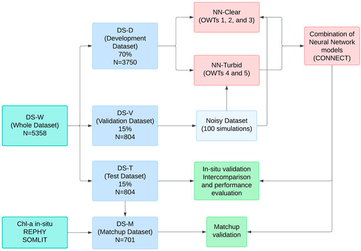
Figure 1. Flowchart of the methodological framework showing the development and validation process of the combined Chl-a model.

2.1 In-situ dataset

The in-situ dataset (used as a training and validation dataset for the Chl-a inversion model development) is composed of different data subsets including (Tran et al., 2023; Lehmann et al., 2023; Valente et al., 2022; Oliveira et al., 2016). The geographical distribution of the in-situ measurements (Figure 2) includes very contrasted water bodies in terms of optical properties as illustrated by the coverage of five OWTs implying clear to ultra-turbid waters previously defined in (Tran et al., 2023). The sampling locations encompass diverse eutrophic states and turbidity levels of the aquatic ecosystems including inland, coastal, and open ocean environments worldwide distributed.

Figure 2

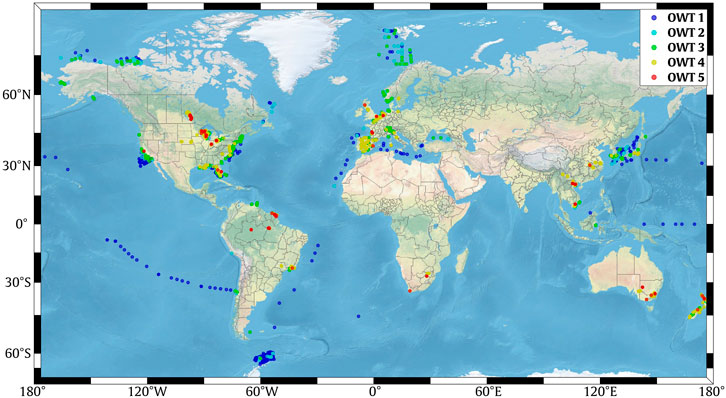
Figure 2. Spatial distribution of the whole in-situ dataset (DS-W) gathering simultaneous Chl-a and radiometric measurements.

Following a standard quality control procedure documented in (Lehmann et al., 2023; Tran et al., 2023), which accounts for the flagged measurements (e.g., noisy and negative spectra, uncertain samples, etc.), this dataset contains 5,358 paired observations of both radiometric hyperspectral and multispectral remote sensing reflectance (R_rs) and surface Chl-a concentrations ranging from 0.017 to 838.24 µg.L^-1 with an average of 17.67 µg.L^-1. The summary statistics of the in-situ Chl-a is provided in Table 1.

Table 1

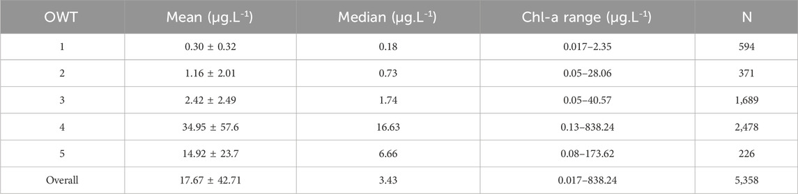
Table 1. Summary statistics of the in-situ Chlorophyll-a dataset across five OWTs.

The whole dataset (DS-W) was randomly partitioned into three subsets: (1) a development dataset (DS-D, 70%) for training; (2) a validation dataset (DS-V, 15%) for generating noise simulations to perform the atmospheric sensitivity validation of the two neural network models; and (3) a test dataset (DS-T, 15%) serving as an independent dataset for evaluating the developed Chl-a model against existing inversion algorithms (Figures 1, 3).

Figure 3

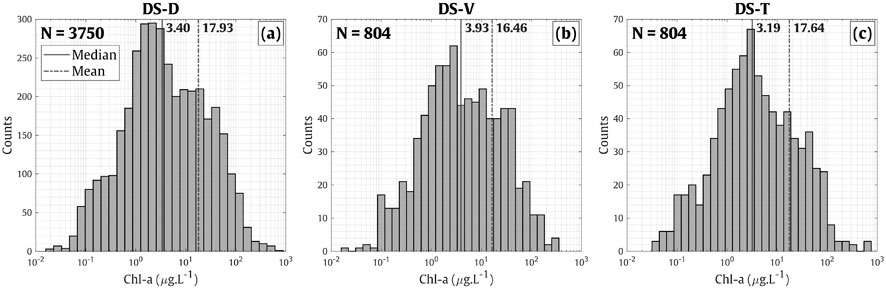
Figure 3. Frequency distribution of the Chl-a concentration on (a) the development dataset (DS-D), (b) the validation dataset (DS-V), and (c) the test datasets (DS-T).

2.2 Matchup dataset

A matchup dataset (DS-M) was constructed by integrating exclusively in-situ Chl-a measurements from the (Lehmann et al., 2023; Valente et al., 2022) datasets for which the corresponding radiometric data for MODIS-A wavebands are not available (these data points are not included in the DS-D and DS-V), and additional Chl-a samples from the long lasting data collected in the framework of French monitoring programs including the Network Monitoring Phytoplankton (REPHY, https://www.seanoe.org/data/00361/47248) and Coastal Environment Observation Service (SOMLIT, https://www.somlit.fr/en/) (Figure 4). To ensure the robustness of the evaluation, the DS-M and DS-T are independent from the development of the algorithm and have in common 228 data points.

Figure 4

Figure 4. Spatial distribution of the Matchup Dataset (DS-M).

In this matchup validation, the daily level L1A MODIS-A archives with 1 × 1 km² spatial resolution of visible wavebands were collected from the database of Ocean Biology Processing Group of National Aeronautics and Space Administration (OBPG of NASA, https://oceandata.sci.gsfc.nasa.gov/) according to the dates and times when in-situ measurements were acquired. Here, we utilized two atmospheric correction (AC) processors including Ocean Color - Simultaneous Marine and Aerosol Retrieval Tool (OC-SMART) (Fan Y. et al., 2021) and Sea, earth, atmosphere Data Analysis System (SeaDAS) to retrieve Level-2 R_rs data. The selection of these processors in the present study is based on their specific advantages. The SeaDAS processor, developed and officially supported by NASA, implements the traditional ocean color approach (Mobley et al., 2016) and is known as the standard atmospheric correction for MODIS-A. On the other hand, OC-SMART, employing MLP neural networks, appears to be a promising machine-learning-based model for retrieving R_rs from satellite data in optically complex environments (Bui et al., 2022; Valerio et al., 2024).

In practice, to perform the matchup validation analysis, the collected in-situ datasets were matched with corresponding MODIS-A satellite images to extract data from a 3 × 3-pixel window centered on the in-situ measurements. The selection of matchup data was controlled using a standard protocol (Werdell et al., 2009) including the following criteria:

• The time difference between the satellite observations and the in-situ data collection was limited to less than 3 h.

• The coefficient of variation (CV) within each 3 × 3-pixel window was kept below 30%. This threshold was established to ensure the spatial homogeneity of the satellite data.

• The matchup extraction process also requires that the number of valid pixels within each 3 × 3-pixel window is spatially representative defining a limit of at least five valid pixels.

The median value of all valid pixels was then calculated for the matchup exercise. In addition, these criteria were applied specifically to the R_rs at 547 nm, as the retrieved errors are typically lowest at this band due to its less absorption by water constituents compared to those in blue or red regions (Goyens et al., 2013; Jamet et al., 2011; Mograne et al., 2019). After applying these selection criteria, the resulting dataset consists of 701 data points, as shown in Figure 4, with Chl-a concentrations ranging from 0.029 to 119.724 µg.L^-1 with an average of 6.88 ± 15.643 µg.L^-1.

2.3 Historical Chlorophyll-a algorithms

2.3.1 OC3M algorithm

The OC3M algorithm is an empirical algorithm with adapted wavebands of MODIS-A sensor. This Chl-a model is developed based on the relationship between the maximum band ratio (MBR) of the blue-to-green reflectance (Equation 2) and Chl-a through a fourth-order polynomial function (Equation 1) (O’Reilly et al., 1998). The updated coefficients and the formulation of the OC3M algorithm follow the recent study by (O’Reilly and Werdell, 2019) and can be described as below:

$\text{Chl}-\mathrm{a}={10}^{{\mathrm{a}}_0+{\mathrm{a}}_1\times \mathrm{R}+{\mathrm{a}}_2\times {\mathrm{R}}^2+{\mathrm{a}}_3\times {\mathrm{R}}^3{+\mathrm{a}}_4\times {\mathrm{R}}^4}(1)$

where

${\mathrm{R}=\log }_{10}\left(\frac{\max \left({\mathrm{R}}_{\text{rs}}\left(442\right),{\mathrm{R}}_{\text{rs}}\left(488\right)\right)}{{\mathrm{R}}_{\text{rs}}\left(547\right)}\right)(2)$

The coefficients for this model are a₀ = 0.26294, a₁ = − 2.64669, a₂ = 1.28364, a₃ = 1.08209, a₄ = − 1.76828.

2.3.2 OC5-Gohin algorithm

The OC5-Gohin model refers to a five-channel model introduced in (Gohin et al., 2002), which was designed to correct the overestimation of Chl-a estimated by the OC4 model (O’Reilly et al., 1998) over coastal environments with the presence of moderately turbid conditions associated with high CDOM levels. This model relies on sensor-specific look-up tables (LUTs) developed from an extensive in-situ dataset to empirically retrieve Chl-a.

2.3.3 MuBR algorithm

The MuBR model is a band-ratio-based algorithm recently proposed by (Tran et al., 2023) to retrieve Chl-a for Sentinel-2/MSI and Sentinel-3/OLCI. In this study, the coefficients of this algorithm were re-tuned for MODIS-A sensor by considering an additional band ratio of reflectance between the red and NIR spectral bands. The model (Equation 3) incorporates four band ratios (Equations 4–7) that capture different spectral signatures across the visible and NIR spectrum.

${\text{Chl}}_{\text{MuBR}}={10}^{{\mathrm{a}}_0+{\mathrm{a}}_1\mathrm{R}1+{\mathrm{a}}_2\mathrm{R}2+{\mathrm{a}}_3\mathrm{R}3+{\mathrm{a}}_4\mathrm{R}4}(3)$

where

$\mathrm{R}1={\log }_{10}\left(\frac{{\mathrm{R}}_{\text{rs}}\left(488\right)}{{\mathrm{R}}_{\text{rs}}\left(442\right)}\right)(4)$

$\mathrm{R}2={\log }_{10}\left(\frac{{\mathrm{R}}_{\text{rs}}\left(547\right)}{{\mathrm{R}}_{\text{rs}}\left(488\right)}\right)(5)$

$\mathrm{R}3={\log }_{10}\left(\frac{{\mathrm{R}}_{\text{rs}}\left(667\right)}{{\mathrm{R}}_{\text{rs}}\left(547\right)}\right)(6)$

$\mathrm{R}4={\log }_{10}\left(\frac{{\mathrm{R}}_{\text{rs}}\left(748\right)}{{\mathrm{R}}_{\text{rs}}\left(667\right)}\right)(7)$

and a₀ = 1.4203, a₁ = −3.2205, a₂ = 2.4194, a₃ = 0.5486, a₄ = 0.3391.

2.4 Multinomial Logistic Regression (MLR)

Multinomial Logistic Regression (MLR) (Hausman and Wise, 1978) is a supervised classification approach used to predict categorical outcomes from one or more independent variables. In this study, we employed MLR to associate each observation with to the corresponding OWT, where the categorical outcomes are the defined OWTs, and the independent variables are the normalized R_rs (${\mathrm{R}}_{\text{rs}}^{\text{norm}}$) values at different wavelengths. The MLR model estimates the log-odds values (Equation 8) corresponding to each OWT through a fitting process in the log-odd transformed axis. The log-odds for OWT_i can be expressed using the following equation:

${\mathrm{Z}}_{\mathrm{i}}={\mathrm{\beta }}_{\mathrm{i}0}+{\mathrm{\beta }}_{\mathrm{i}1}{\mathrm{X}}_1+{\mathrm{\beta }}_{\mathrm{i}2}{\mathrm{X}}_2+\dots +{\mathrm{\beta }}_{\text{in}}{\mathrm{X}}_{\mathrm{n}}(8)$

where ${\mathrm{Z}}_{\mathrm{i}}$ is the log-odd values of OWT_i, n is the number of spectral bands involved in the classification, ${\mathrm{\beta }}_{\mathrm{i}0}$, ${\mathrm{\beta }}_{\mathrm{i}1}$,…, ${\mathrm{\beta }}_{\text{in}}$ are the optimized coefficients, and X₁, X₂, … , X_n are the independent variables (${\mathrm{R}}_{\text{rs}}^{\text{norm}}$). The coefficients are estimated through an iterative process to maximize the likelihood function (Murphy, 2012).

Once the log-odds are obtained, the probability P_i(X) of a given data point to belong to the OWT_i can be then computed through softmax normalization (Equation 9):

${\mathrm{P}}_{\mathrm{i}}\left(\mathrm{X}\right)=\frac{{\mathrm{e}}^{{\mathrm{z}}_{\mathrm{i}}}}{{\displaystyle {\sum }_{\mathrm{j}}^{\mathrm{K}}}{\mathrm{e}}^{{\mathrm{z}}_{\mathrm{j}}}}(9)$

where K is the total number of defined OWTs, ${\mathrm{e}}^{{\mathrm{z}}_{\mathrm{i}}}$ is the exponentiated log-odds for OWT_i, and ${\sum }_{\mathrm{j}}^{\mathrm{K}}{\mathrm{e}}^{{\mathrm{z}}_{\mathrm{j}}}$ is the sum of the exponentiated log-odds for all OWTs. Each observation is then assigned to the OWT according to the highest probability yielded from the MLR.

2.5 Multi-Layer Perceptron (MLP)

Multi-Layer Perceptron (MLP) is a type of Artificial Neurals Networks (ANNs) that is particularly effective in solving regression problems. Its application has immensely contributed to the facilitation of intricate and non-linear patterns in the data in various practical scenarios, including those related to the field of ocean color remote sensing (D’Alimonte and Zibordi, 2003; Doerffer and Schiller, 2007; Gross et al., 2000; Jamet et al., 2012; Rubbens et al., 2023). The architecture of an MLP typically involves an input layer (here the MODIS-A R_rs), one or more hidden layers, and an output layer (Chl-a). Each layer is composed of fully connected neurons through adjustable weights. These weights or connections are optimized as the network is trained through an iterative back-propagation process (Bishop, 1995).

In regression tasks, the input layer captures the input data of independent variables, which is then passed and processed through the hidden layers. Each neuron in these layers employs an activation function on its inputs, allowing the network to learn complex features of the data (Bishop and Nasrabadi, 2006). The output layer subsequently produces continuous output values, representing the prediction from MLP. During the training process, the MLP adjusts weights of the neural network to minimize the error between the it’s prediction and the actual data, which is typically calculated through a loss function (Bishop and Nasrabadi, 2006).

Historical neural network approaches to retrieve Chl-a have typically relied on a single model to estimate the entire range of Chl-a (Chen et al., 2024; D’Alimonte and Zibordi, 2003; Pahlevan et al., 2020). In an effort to better exploit the advantages of machine learning, this study contributes to the optimization of Chl-a retrievals from satellite data through the development and combination of MLP models. This combination was performed by using the weights for different groups of OWTs with the aim to obtain more accurate and seamless Chl-a estimates across various trophic conditions.

2.6 Statistic indicators

To evaluate the performance of the considered models, we adopted a set of statistical indicators computed between in-situ observations and model-derived estimates. The computation of these performance metrics can be expressed as follows:

${\mathrm{R}}_{\log }^2=1-\frac{{\displaystyle {\sum }_{\mathrm{i}}^{\mathrm{N}}}{\left({\log }_{10}\left({\mathrm{y}}_{\mathrm{i}}^{\text{obs}}\right)-{\log }_{10}\left({\mathrm{y}}_{\mathrm{i}}^{\mathrm{mod}}\right)\right)}^2}{{\displaystyle {\sum }_{\mathrm{i}}^{\mathrm{N}}}{\left({\log }_{10}\left({\mathrm{y}}_{\mathrm{i}}^{\text{obs}}\right)-\frac{1}{\mathrm{N}}{\displaystyle {\sum }_{\mathrm{i}=1}^{\mathrm{N}}}{\log }_{10}\left({\mathrm{y}}_{\mathrm{i}}^{\text{obs}}\right)\right)}^2}(10)$

${\text{Slope}}_{\log }=\sqrt[2]{\begin{array}{c}\left(\frac{{\displaystyle {\sum }_{\mathrm{i}=1}^{\mathrm{N}}}\left({\log }_{10}\left({\mathrm{y}}_{\mathrm{i}}^{\text{obs}}\right)-\overline{{\log }_{10}\left({\mathrm{y}}_{\mathrm{i}}^{\text{obs}}\right)}{\left)\times (\log \right.}_{10}\left({\mathrm{y}}_{\mathrm{i}}^{\mathrm{mod}}\right)-\overline{{\log }_{10}\left({\mathrm{y}}_{\mathrm{i}}^{\mathrm{mod}}\right)}\right)}{{\displaystyle {\sum }_{\mathrm{i}=1}^{\mathrm{N}}}{\left({\log }_{10}\left({\mathrm{y}}_{\mathrm{i}}^{\text{obs}}\right)-\overline{{\log }_{10}\left({\mathrm{y}}_{\mathrm{i}}^{\text{obs}}\right)}\right)}^2}\right)\\ \times \left(\frac{{\displaystyle {\sum }_{\mathrm{i}=1}^{\mathrm{N}}}\left({{\log }_{10}\left({\mathrm{y}}_{\mathrm{i}}^{\mathrm{mod}}\right)-\overline{{\log }_{10}\left({\mathrm{y}}_{\mathrm{i}}^{\mathrm{mod}}\right)})\times (\log }_{10}\left({\mathrm{y}}_{\mathrm{i}}^{\text{obs}}\right)-\overline{{\log }_{10}\left({\mathrm{y}}_{\mathrm{i}}^{\text{obs}}\right)}\right)}{{\displaystyle {\sum }_{\mathrm{i}=1}^{\mathrm{N}}}{\left({\log }_{10}\left({\mathrm{y}}_{\mathrm{i}}^{\mathrm{mod}}\right)-\overline{{\log }_{10}\left({\mathrm{y}}_{\mathrm{i}}^{\mathrm{mod}}\right)}\right)}^2}\right)\end{array}}(11)$

$\text{MAPD}=\text{median}\left(\frac{\left|{\mathrm{y}}^{\mathrm{mod}}-{\mathrm{y}}^{\text{obs}}\right|}{{\mathrm{y}}^{\text{obs}}}\right)\times 100\%(12)$

$\text{SSPB}=\text{sign}\left(\text{median}\left(\frac{{\log }_{10}\left({\mathrm{y}}^{\mathrm{mod}}\right)}{{\log }_{10}\left({\mathrm{y}}^{\text{obs}}\right)}\right)\right)\times \left({10}^{\left|\text{median}\left(\frac{{\log }_{10}\left({\mathrm{y}}^{\mathrm{mod}}\right)}{{\log }_{10}\left({\mathrm{y}}^{\text{obs}}\right)}\right)\right|}-1\right)\times 100\%(13)$

where ${\mathrm{y}}^{\text{obs}}$ represents the in-situ observations and ${\mathrm{y}}^{\mathrm{mod}}$ is the model-derived estimates. ${\mathrm{R}}_{\log }^2$ and ${\text{Slope}}_{\log }$ are the determination coefficient and the Slope of type II regression calculated from the logtransformed data, respectively (Equations 10, 11). MAPD represents Median Absolute Percentage Difference computed in linear scale and SSPB stands for Symmetric Signed Percentage Bias (Equations 12, 13). Here, we also used the radar chart derived from the normalized values (Equations 14-18) of the mentioned metrics and the number of not valid (NV) data points that a model can output to assess the performance of the candidate model j (Nguyen et al., 2024; Tran et al., 2023).

${\mathrm{R}}_{\text{norm}}^2\left(\mathrm{j}\right)=\frac{\min \left({\mathrm{R}}_{\log }^2\left(\mathrm{j}\right),\mathrm{j}=1,\mathrm{k}\right)}{{\mathrm{R}}_{\log }^2\left(\mathrm{j}\right)}(14)$

${\text{Slope}}_{\text{norm}}\left(\mathrm{j}\right)=\frac{\left|1-{\text{Slope}}_{\log }\left(\mathrm{j}\right)\right|}{\max \left(\left|1-{\text{Slope}}_{\log }\left(\mathrm{j}\right)\right|,\mathrm{j}=1,\mathrm{k}\right)}(15)$

${\text{MAPD}}_{\text{norm}}\left(\mathrm{j}\right)=\frac{\text{MAPD}\left(\mathrm{j}\right)}{\max \left(\text{MAPD}\left(\mathrm{j}\right),\mathrm{j}=1,\mathrm{k}\right)}(16)$

${\text{SSPB}}_{\text{norm}}\left(\mathrm{j}\right)=\frac{\left|\text{SSPB}\left(\mathrm{j}\right)\right|}{\max \left(\left|\text{SSPB}\left(\mathrm{j}\right)\right|,\mathrm{j}=1,\mathrm{k}\right)}(17)$

${\text{NV}}_{\text{norm}}\left(\mathrm{j}\right)=\frac{\text{NV}\left(\mathrm{j}\right)}{\max \left(\text{NV}\left(\mathrm{j}\right),\mathrm{j}=1,\mathrm{k}\right)}(18)$

The area computed from the radar chart, (Equation 19) denoted as ${\text{area}}_{\text{norm}}$, will then be used as a score metric to rank the accuracy of the inversion algorithms considered in the inter-comparison. A lower ${\text{area}}_{\text{norm}}$ indicates better overall algorithm performance, as it represents smaller errors across all statistical indicators. This metric represents the synthetic information of the five mentioned statistical indicators and can be computed as:

${\text{area}}_{\text{norm}}=\frac{1}{2}\times \frac{\mathrm{\pi }}{5}\times \left[{\mathrm{R}}_{\text{norm}}^2\left(\mathrm{j}\right)\times {\text{Slope}}_{\text{norm}}\left(\mathrm{j}\right)+{\text{Slope}}_{\text{norm}}\left(\mathrm{j}\right)\times {\text{MAPD}}_{\text{norm}}\left(\mathrm{j}\right)+{\text{MAPD}}_{\text{norm}}\left(\mathrm{j}\right)\times {\text{SSPB}}_{\text{norm}}\left(\mathrm{j}\right)+{\text{SSPB}}_{\text{norm}}\left(\mathrm{j}\right)\times {\text{NV}}_{\text{norm}}\left(\mathrm{j}\right)+{\text{NV}}_{\text{norm}}\left(\mathrm{j}\right)\times {\mathrm{R}}_{\text{norm}}^2\right](19)$

3 Results and discussion

3.1 Development of CONNECT algorithm

In response to the challenges posed by differences in optical properties between Case-1 and Case-2 waters as aforementioned, adopting and/or merging multiple bio-optical models along with the use of appropriate blending approaches have proven the effectiveness in better retrieving precise information about water constituents such as SPM (i.e., Han et al., 2016) and Chl-a (i.e., Lavigne et al., 2021; Smith et al., 2018). This adaptive approach, which applies different bio-optical algorithms based on their performance in specific water types, allows more precise quantification of water constituents across diverse aquatic environments (Stramski et al., 2023).

The principle of developing multiple neural network models or ensemble learning for solving regression problems relies on its advantages to optimize the accuracy and robustness compared to a single model as each model can capture different aspects of the data and eventually mitigate individual model biases and errors (Moreira et al., 2012; Yang et al., 2013). This is also demonstrated through the results obtained from our initial test where the combination of the two neural network models, tailored to different groups of OWTs exhibits an improvement compared to the case of a single model trained on the entire in-situ dataset.

For this reason, the first model, referred to as ‘NN-Clear’, was trained to specifically estimate Chl-a over clear to moderately turbid waters. This model requires R_rs at six MODIS-A visible bands (412 nm, 443 nm, 488 nm, 531 nm, 547 nm, and 667 nm) as the inputs. Here, R_rs (748) was excluded from the NN-Clear model since water-leaving radiance at NIR wavelengths is typically negligible in open ocean waters, following the black pixel assumption (Gordon and Wang, 1994; Goyens et al., 2013). The second model (NN-Turbid) is designed particularly for turbid and ultra-turbid waters with parameterization of seven variables including R_rs values at six MODIS-A visible bands and the NIR band at 748 nm. In addition, we also considered the OWT-specific probability in the development of each neural network model to ensure the spatial continuity in the Chl-a maps.

3.1.1 Optical water type labelling technique

In this study, we further extend the work done by (Tran et al., 2023), in which OWTs 1 to 3 were identified as clear to moderately turbid waters, while OWTs 4 and 5 are related to higher level of Chl-a and SPM, typically associated with coastal and inland waters. To retrieve the OWTs, an MLR model was established using the same training dataset of the 5 OWTs used in (Tran et al., 2023), with a specific adaptation considering the spectral bands of MODIS-A sensor. Such method was applied to the normalized R_rs (${\mathrm{R}}_{\text{rs}}^{\text{norm}}$) to obtain the probability values that represent the degree of membership to each OWT as detailed in section 2.4. In this way, the model provides information about the confidence level of a given pixel or data point to belong to each defined OWT, which is valuable for the model training and merging processes. In addition, our tests suggest that the MLR approach can provide relatively balanced probability values, which is theoretically beneficial to produce fine gradient in the transition zone where one algorithm switches to another.

3.1.2 Development of two neural network models

The data preprocessing step involves the division of the DS-W into DS-D and DS-V for development and validation purposes (see section 2.1). Then, we applied the z-score standardization technique on the input R_rs data using a standard scaler as it is less sensitive to outliers compared to the min-max normalization method (Fan C. et al., 2021). This data transformation step is crucial for accelerating training convergence as well as enhancing overall model performance (Ioffe and Szegedy, 2015; Jamet et al., 2012, Jamet et al., 2005; Jamet et al., 2004). The z-score standardization of the input R_rs (λ) can be expressed as in the following equation:

${{\mathrm{R}}_{\text{rs}}\left(\mathrm{\lambda }\right)}_{\text{scaled}}=\frac{{\mathrm{R}}_{\text{rs}}\left(\mathrm{\lambda }\right)-\mathrm{\mu }}{\mathrm{\sigma }}(20)$

where R_rs (λ)_scaled is the scaled Rrs at the wavelength λ (nm), R_rs (λ) is the raw input reflectance, µ is the mean, and σ is the standard deviation of the input R_rs data (Equation 20). Besides, we also applied a logarithmic transformation to the Chl-a data for two keys reasons: 1) Chl-a concentrations in natural waters tend to follow a lognormal distribution (Campbell, 1995; Mélin and Vantrepotte, 2015). 2) log-transforming the data allows for a more effective training process (Feng et al., 2014).

The training process was implemented using Adaptive Moment Estimation (ADAM) optimizer (Kingma and Ba, 2017) available within the tensorflow library for machine learning in Python (Raschka and Mirjalili, 2019). Here, we used the Neural Architecture Search (NAS) technique where the number of hidden layers and the associated neurons of the MLP were dynamically tested along with the iterative adjustments of the L2 regularization values (Neumaier, 1998) to avoid the risk of getting an over-fitting issue. The Rectified Linear Unit (ReLU) activation function was employed to transform the propagated data in each hidden layer, allowing the network to learn complex patterns of the data (Agarap, 2019). To further improve the model’s predictive consistency across diverse aquatic environments, we also adopted dropout and early stopping techniques during the training phase (Prechelt, 1998). The objective of this comprehensive training procedure is to generate a set of candidate models, which were then evaluated to select the most pertinent MLP model to predict Chl-a concentrations. To accomplish this, we incorporated random Gaussian noise into the validation dataset through 100 simulations following the work of (Nguyen et al., 2024) to simulate the uncertainties stemming from atmospheric disturbances based on the mean MAPD values derived from the in-situ and satellite-derived R_rs matchups of OC-SMART and SeaDAS AC algorithms (see Table 3). Then, these noise-augmented datasets were then used as indicators for the sensitivity assessment where the model yielded the lower standard deviation value on the simulated noisy datasets exhibits lower sensitivity to atmospheric interference.

The selection of model architectures for NN-Clear and NN-Turbid models was performed independently through the NAS process, which objectively identifies the optimal number of layers and neurons from the prediction error on the DS-V. The NAS algorithm determined that NN-Turbid required a deeper architecture (three hidden layers with 17, 8, and 4 neurons) compared to NN-Clear (two hidden layers with 12 and 6 neurons) due to the greater complexity of the regression problem for OWTs 4 and 5, which represent turbid and ultra-turbid waters. In these conditions, the relationships between R_rs and Chl-a are typically influenced by optical contributions from other co-existing constituents such as suspended sediments and CDOM, making the retrieval of Chl-a more challenging. The increased architectural complexity of the NN-turbid reflects the need for a more complex neural network to accurately estimate Chl-a in optically complex environments, while a simpler network suffices for the case of clear to medium turbid waters (OWTs 1–3) where the optical signal is mainly driven by phytoplankton biomass.

To ensure the complementarity of the two MLP models, while allowing the possibility for each model to specialize in one group of OWTs, we incorporated weights corresponding to the probability of belonging to each group of OWTs in the loss function (see Equation 9; Equation 21). More specifically, the NN-Clear model was trained on the entire DS-D with the incorporation of the probability values corresponding to OWTs 1, 2, and 3, whereas the NN-Turbid model was trained by considering of the probability values for OWTs 4 and 5. The integration of OWT-specific probability values into the loss function allows each model to optimize its performance in its designated water types while preserving gradual transitions between two OWT groups. As a result, this helps to avoid the spatial discontinuity issue potentially appears in the Chl-a map when combining multiple inversion models.

Thus, the mathematical formulation of the loss function, ${\mathrm{L}}_{\text{weighted}}$, for the training process is defined as:

${\mathrm{L}}_{\text{weighted}}=\frac{1}{\mathrm{N}}{\displaystyle \sum _{\mathrm{i}=1}^{\mathrm{n}}}\mathrm{P}\times {\left({\mathrm{y}}_{\mathrm{i}}^{\mathrm{mod}}-{\mathrm{y}}_{\mathrm{i}}^{\text{obs}}\right)}^2(21)$

where p is the probability values for the designated group of OWTs (e.g., $\mathrm{P}={\mathrm{p}}_1+{\mathrm{p}}_2+{\mathrm{p}}_3$ for NN-Clear and $\mathrm{P}={\mathrm{p}}_4+{\mathrm{p}}_5$ for NN-Turbid, in which ${\mathrm{p}}_1,{\mathrm{p}}_2,{\mathrm{p}}_3,{\mathrm{p}}_4$, and ${\mathrm{p}}_5$ are the probability values corresponding to the five OWTs) and ${\mathrm{y}}^{\text{obs}}$ represents the in-situ Chl-a observations and ${\mathrm{y}}^{\mathrm{mod}}$ is the model-derived estimates after each training iteration.

The performance of NN-Clear on the DS-D and DS-V is shown in Figure 5 where the Chl-a estimates demonstrate a consistency on both datasets, implying an effective avoidance of overfitting with the approximate MAPD values of 38.58% and 41.69% on the DS-D and DS-V, respectively. Furthermore, the establishment of the NN-Turbid model leads to a good performance on the in-situ dataset, as evidenced by the Slope_log and MAPD values of 0.91% and 38.54% on the DS-V (Figure 6b). The inclusion of the OWT 4 and OWT 3 data points for the NN-Clear and NN-Turbid models, respectively, in the scatterplots is to ensure that our trained models did not result in any artificial saturation effects at the boundaries with the complementary OWT group, demonstrating the effectiveness of incorporating probability values in the loss function.

Figure 5

Figure 5. Relationship between the in-situ vs. estimated Chl-a from the NN-Clear model on the in-situ observations corresponding to OWTs 1, 2, 3, and 4 in (a) the DS-D dataset (N = 3,596) and (b) the DS-V dataset (N = 764).

Figure 6

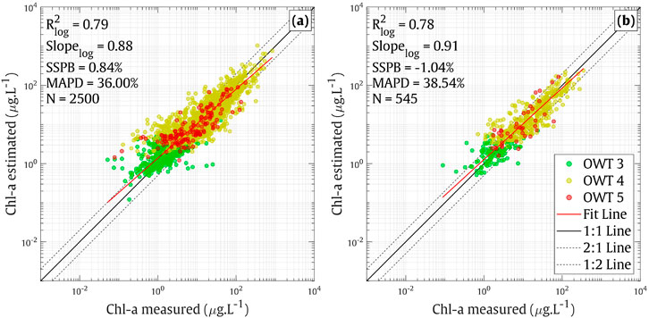
Figure 6. Relationship between the in-situ vs. estimated Chl-a from the NN-Turbid model on the in-situ observations corresponding to OWTs 3, 4 and 5 in (a) the DS-D dataset (N = 2,500) and (b) the DS-V dataset (N = 545).

3.1.3 Combination of two neural network models

The combination of the two trained neural network models for estimating Chl-a was conducted using the sum of the probability values corresponding to each group of OWTs obtained from the MLR model. In this way, the CONNECT model presented here, utilizes these probability values as the blending coefficients to perform the algorithm merging process, which can be expressed in the following equation:

$\text{Chl}-\mathrm{a}=\left({\mathrm{p}}_1+{\mathrm{p}}_2+{\mathrm{p}}_3\right)\times {\text{Chl}-\mathrm{a}}_{\text{clear}}+\left({\mathrm{p}}_4+{\mathrm{p}}_5\right)\times {\text{Chl}-\mathrm{a}}_{\text{turbid}}(22)$

where ${\mathrm{p}}_1$, ${\mathrm{p}}_2$, ${\mathrm{p}}_3$, ${\mathrm{p}}_4$, and ${\mathrm{p}}_5$ are the probability values corresponding to the five OWTs (see section 2.5), ${\text{Chl}-\mathrm{a}}_{\text{clear}}$ and ${\text{Chl}-\mathrm{a}}_{\text{turbid}}$ are the Chl-a estimates obtained from the NN-Clear and NN-Turbid models, respectively (see section 3.1.1). In practice, for any given water pixel, the MLR model assigns probability values (${\mathrm{p}}_1$ to ${\mathrm{p}}_5$) to the five predefined OWTs. These probabilities represent the likelihood of the water pixel to belong to one of the OWTs, with the sum equals to 1 (or 100%). Then, the two MLP models NN-Clear and NN-Turbid independently estimate the Chl-a concentration (${\text{Chl}-\mathrm{a}}_{\text{clear}}$ and ${\text{Chl}-\mathrm{a}}_{\text{turbid}}$) for the same pixel. However, instead of simply choosing one estimate over the other, the model used a weighted average based on the water type probabilities (Equation 22). The primary objective of this combination process is to incorporate the Chl-a estimates from both MLP models without introducing artificial discontinuity in the final Chl-a maps. Consequently, the approach maintains a smooth spatial transition between different water conditions, resulting in a more realistic representation of the Chl-a distribution across multiple OWTs.

3.2 Intercomparison and performance evaluation

The inter-comparison of the accuracy of Chl-a retrievals for MODIS-A sensor between CONNECT and the historical algorithms on the in-situ DS-V is illustrated in Figure 7. The estimated Chl-a for each model is calculated according as described in section 2.3. More detailed information about the statistical metrics (see section 2.4) for each considered Chl-a model with respect to five OWTs is presented in Table 2.

Figure 7

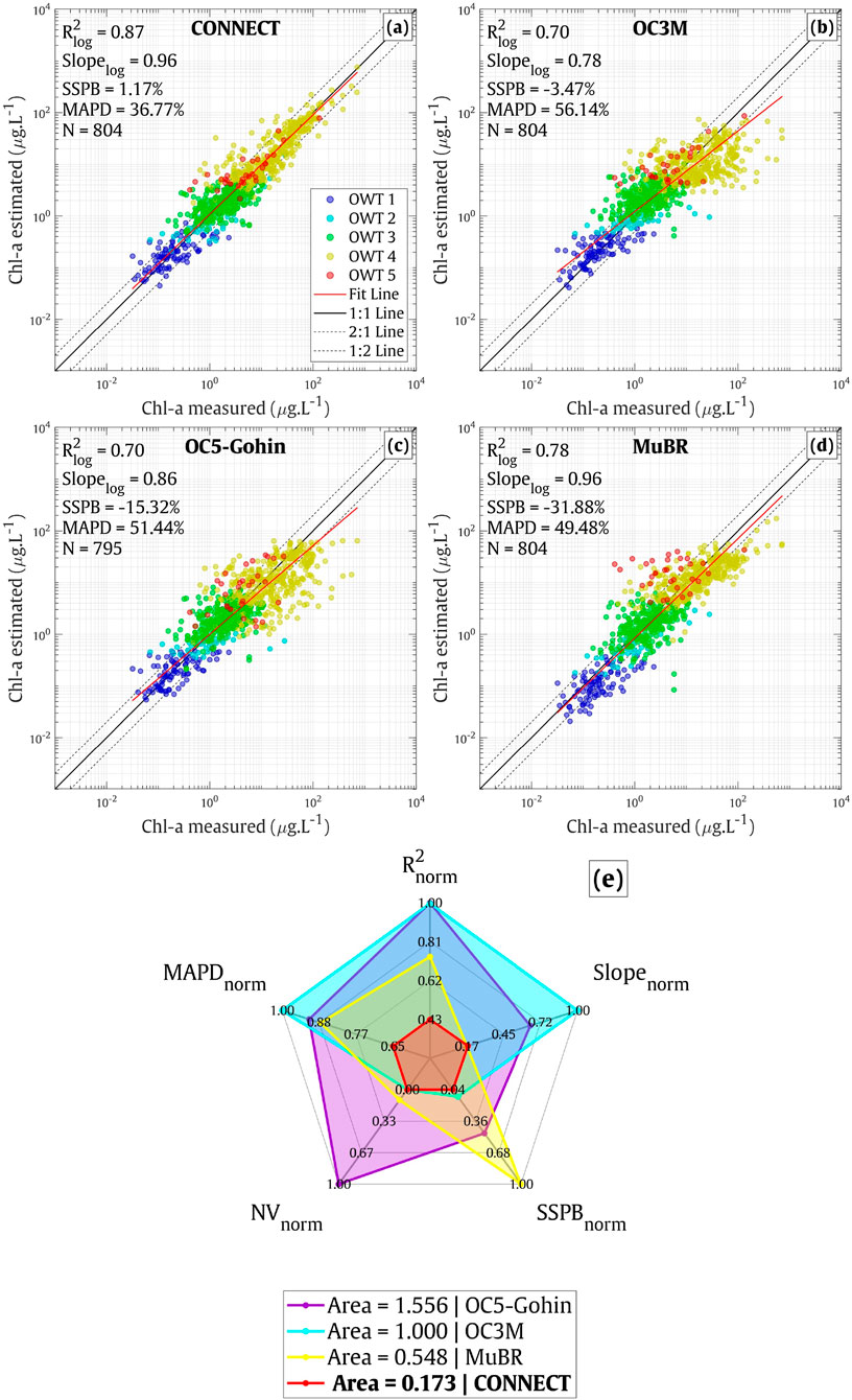
Figure 7. Scatterplots (log–log scale) of the in-situ Chl-a (DS-T) vs. Chl-a estimated from different Chl-a models (a) CONNECT, (b) OC3M, (c) OC5-Gohin, (d) MuBR. (e) Summary of the performance of the Chl-a inversion models where the lowest area of the polygon associated with each model represented in the radar plot corresponds to the best model.

Table 2

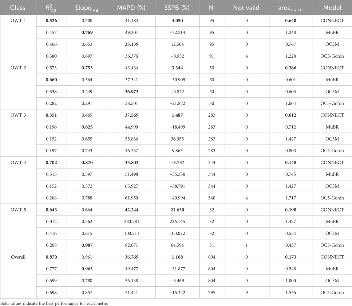
Table 2. Statistical indicators evaluating the Chl-a retrieval performance of the CONNECT model vs. the 3 Blue/Green models: OC5-Gohin, OC3M, and MuBR. The metrics were computed using in-situ DS-T Chl-a measurements and model-derived estimates over the five OWTs.

The results obtained from this investigation show that the CONNECT model generally outperforms the existing models, as evidenced by the smallest area (0.173) on the radar chart as well as its superior performance found for all metrics considering the entire DS-T. The scatterplots in Figures 7b–d further emphasize the lower performance of typical Blue/Green algorithms (i.e., OC3M, OC5-Gohin) over turbid coastal and inland waters, indicated by higher uncertainties associated with OWTs 4 and 5 (Table 2). This finding aligns with previous studies as the Blue/Green approaches are better suited to offshore clear environments where the optical signal is dominated by phytoplankton pigments (Dierssen and Karl, 2010; Neil et al., 2019; Tran et al., 2023). In addition, the OC5-Gohin model appears to be more reliable than the OC3M model in retrieving Chl-a over moderately turbid water (OWT 3) while the opposite situation was found in clearer environments (OWT 2). This difference is understandable given that the OC5-Gohin model was specifically adapted for French coastal waters. Although the MuBR model generally yields a satisfactory performance over mesotrophic conditions with a relatively good Slope value of 0.82 recorded for OWT 3, the machine learning-based algorithm introduced in the present study shows clear improvements over all trophic levels in the DS-T, especially for eutrophic waters (OWT 4) where the Chl-a can reach up to 838.236 µg.L^-1. This indicates that the combination of adapted OWT-specific neural network models represents a remarkable enhancement in retrieving Chl-a in our in-situ dataset.

3.3 Matchup analysis

3.3.1 Performance of atmospheric correction methods

Before studying the quality of the Chl-a estimates from MODIS-A sensor, two atmospheric correction algorithms (SeaDAS and OC-SMART) were validated, as shown in Figure 8. The statistical parameters per wavelength are provided in Table 3.

Figure 8

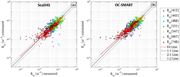
Figure 8. Performance of (a) SeaDAS and (b) OC-SMART AC algorithms to retrieve R_rs on the DS-M (concomitant matchups).

Table 3

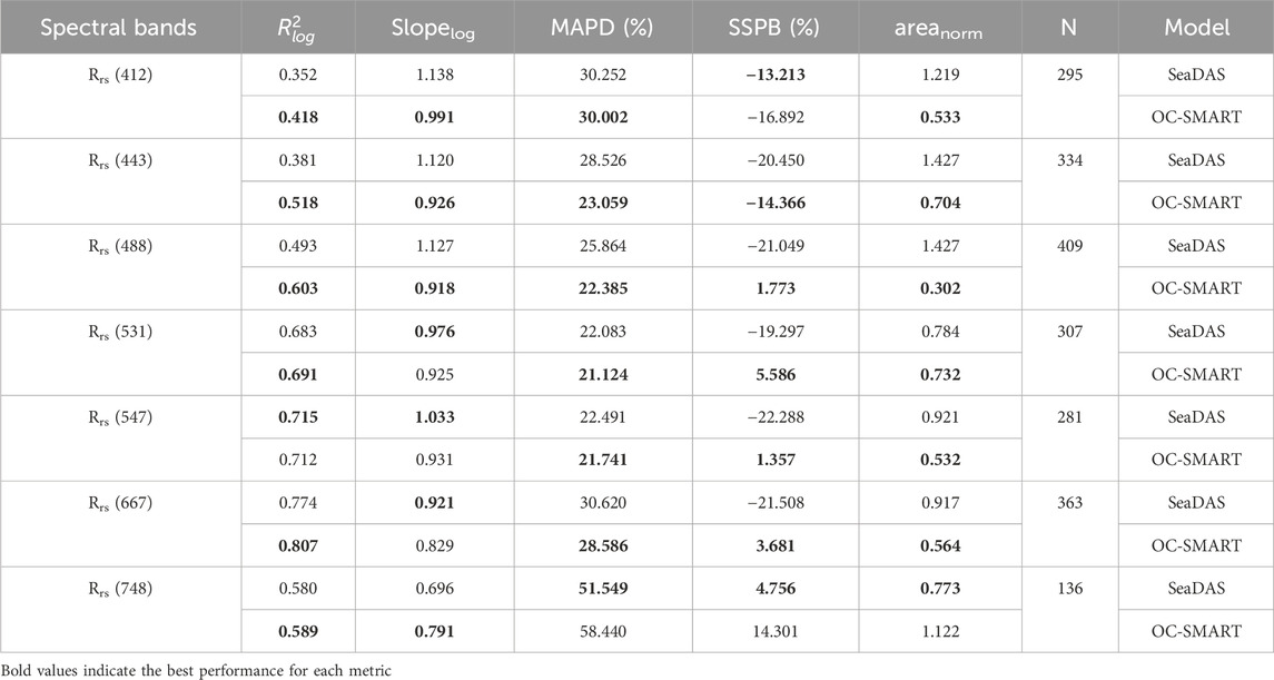
Table 3. Statistical metrics evaluating the R_rs retrieval performance of the SeaDAS and OC-SMART AC processors. The metrics were computed using in-situ R_rs measurements and satellite-derived estimates considering MODIS-A’s spectral bands. The difference in number of data points for each wavelength here is attributed to the availability of our in-situ R_rs measurements.

Although OC-SMART retrieved more matchups without producing negative R_rs compared to SeaDAS (l2gen) (not shown), we only highlighted the analysis on the common matchups to obtain a fair performance evaluation of these two AC processors on the same data samples of 2,125 data points across all considered wavelengths. Scatterplots in Figure 8 indicates that OC-SMART and SeaDAS processors exhibited a fairly comparable accuracy in retrieving R_rs from the TOA signals, evidenced by an approximation in the MAPD values (SeaDAS: 27.8%, OC-SMART: 25.16%). Detailed information about different statistical metrics, considering each individual wavelength as shown in Table 3, generally shows better accuracy of retrieving R_rs in the green bands and a lower performance towards the blue and NIR bands, which is in good agreement with earlier studies (Mograne et al., 2019; Pahlevan et al., 2021). Results from this examination also indicate that OC-SMART exhibits a fairly better performance compared to SeaDAS in the visible spectral bands. The lower performance found for both AC methods at the wavelength of 748 nm emphasizes the need to improve the AC in the NIR domain (Mograne et al., 2019).

3.3.2 Chl-a retrieval accuracy

Although the OC3M model showed limitations to derive accurate Chl-a estimates over coastal turbid environments as shown in our examination on the in-situ observations (see section 3.3.1), this model has been known as one of the standard Chl-a algorithms for MODIS-A and its reliability in terms of accuracy has been extensively evaluated in various studies (Clay et al., 2019; Pereira and Garcia, 2018; Tilstone et al., 2013). Therefore, in this analysis, a cross comparison between OC3M and CONNECT models was performed using the common matchups, defined by simultaneously applying the flags produced by both OC-SMART and SeaDAS AC processors (see section 3.3.1).

The scatterplots in Figures 9a–d illustrate the overall performance of the CONNECT and OC3M models with respect to the two considered AC approaches. The areas in the radar chart Figure 9e) suggest an overall better performance of the machine learning-based approach presented in this work compared to the OC3M Chl-a algorithm considering both clear and turbid environments. This is further illustrated by higher ${\mathrm{R}}_{\log }^2$ values (SeaDAS: 0.85, OC-SMART: 0.83) and Slope_log (SeaDAS: 0.99, OC-SMART: 0.94) and lower values of SSPB (SeaDAS: 11.65%, OC-SMART: 15.71%) for the CONNECT model (N = 701). In addition, the OC3M model produced consistently overestimated Chl-a concentrations for water bodies classified as OWT 3, regardless of the atmospheric correction method applied. The CONNECT model, on the other hand, successfully overcame this overestimation issue and provided more accurate Chl-a retrievals over such moderately turbid waters which is typically associated with coastal environments. This finding aligns with the statistical analysis on our in-situ dataset presented in Table 2, where OWT-3 data points processed by the OC3M model exhibited a remarkably high SSPB value of 36.9%.

Figure 9

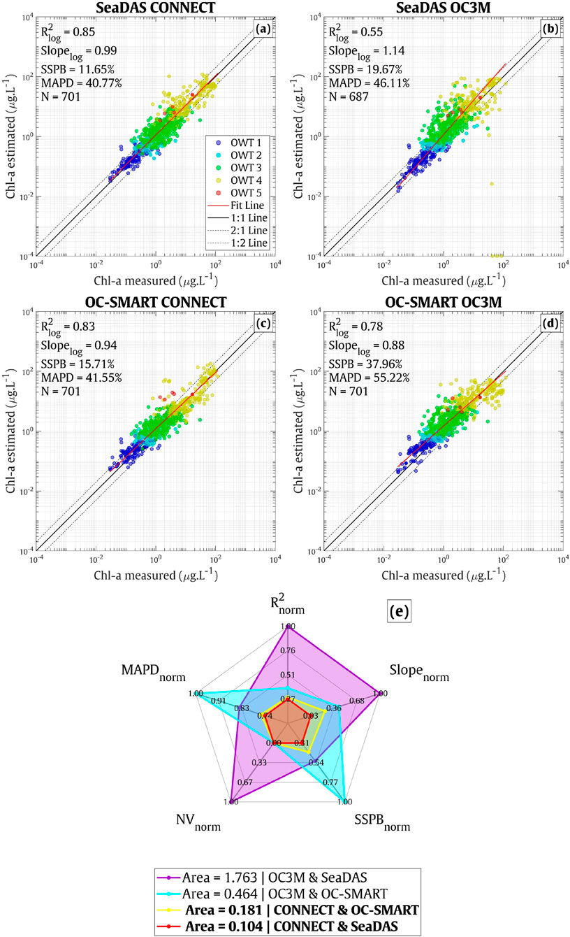
Figure 9. Chl-a matchup validation of the CONNECT (a,c) and OC3M (b,d) models using the Rrs obtained from SeaDAS (a,b) and OC-SMART (c,d) AC processors. (e) Summary radar chart comparing normalized performance metrics.

Regarding clear to moderately turbid waters (OWTs 1, 2, and 3), Chl-a retrievals from R_rs SeaDAS and OC-SMART processing exhibit a comparable accuracy considering both CONNECT and OC3M Chl-a models with fairly approximate ${\mathrm{R}}_{\log }^2$ values (e.g., CONNECT & SeaDAS: 0.73, CONNECT & OC-SMART: 0.72) and MAPD values (e.g., CONNECT & SeaDAS: 40.9%, CONNECT & OC-SMART: 42.8%), respectively. Interestingly, in turbid waters (OWTs 4 and 5), Chl-a estimations obtained from OC-SMART demonstrates a remarkable improvement, emphasizing the reliability of this AC algorithm in turbid coastal environments, evidenced through the recorded SSPB values (CONNECT & OC-SMART: 7.94% vs. CONNECT & SeaDAS: 17.58%) and MAPD values (CONNECT & OC-SMART: 36.58% vs. CONNECT & SeaDAS: 40.47%).

In addition, the result obtained for the CONNECT and OC3M models in extremely turbid waters should be interpreted with caution due to very limited sample size for OWT 5 (only five matchup data points) given the poor performance of the OC3M model in the in-situ dataset for this OWT (see section 3.2; Figure 7). Another explanation is that high uncertainties associated with the retrievals of R_rs in the NIR region particularly at the waveband 748 nm by OC-SMART might contribute to the lower performance of the bio-optical algorithms over such optically complex environments (Pahlevan et al., 2021).

3.4 Visual assessment of Chl-a CONNECT product

To further understand the spatial distribution of Chl-a generated by the CONNECT model as well as its sensitivity to different AC methods on Chl-a products, several MODIS-A scenes covering three different locations were examined across different trophic levels and optical conditions with coastal to offshore gradients associated with multiple OWTs. The selected area were the Guanabara Bay (turbid, ultra-eutrophic waters (Martins et al., 2016; Oliveira et al., 2016)), the English Channel (moderately turbid, mesotrophic waters (Gohin et al., 2020, Gohin et al., 2019)), and the lower Mekong River (ultra-turbid, mesotrophic waters (Loisel et al., 2017, Loisel et al., 2014)). This visual assessment is conducted considering the same inputs with previous sections, where the CONNECT model is compared to OC3M with respect to the SeaDAS and OC-SMART AC processors.

Figure 10 illustrates the MODIS-derived Chl-a products and their corresponding OWTs over the Bay of Rio on 13th July 2019. When comparing the bio-optical algorithms, it is evident that the CONNECT model, paired with the OC-SMART AC method, successfully produces Chl-a products that are more closely aligned with the actual conditions in the Guanabara Bay at approximately 43° W, 23° S where the Chl-a level was recorded up to approximately 500 µg.L^-1 in our in-situ dataset (Oliveira et al., 2016). In contrast, the OC3M model yields lower Chl-a concentrations, suggesting a potential underestimation in its Chl-a retrievals in eutrophic waters as previously observed in the analysis performed on the in-situ dataset (Figure 7). From the MODIS maps Figure 10d and historical research findings, it can be inferred that the results from the CONNECT are more consistent with the documented eutrophic gradient between Guanabara Bay and Sepetiba Bay, with higher Chl-a levels observed in Guanabara Bay (Cotovicz et al., 2018; Rezende et al., 2010). Furthermore, the consistency in the Chl-a distribution derived from the OC3M and CONNECT models, especially in the transition areas between OWTs 3 and 4, confirms a smooth transition where the NN-Clear switches to NN-Turbid (see sections 3.1.1 and 3.1.2). This result demonstrates the spatial effectiveness of using probability values as blending weights to combine multiple bio-optical models, ensuring gradual changes in Chl-a estimations across different water types (Mélin et al., 2011; Tran et al., 2023; Vantrepotte et al., 2012).

Figure 10

Figure 10. Comparison of MODIS-A ocean color data processing methods and their results for the coastal region near the Bay of Rio on 13^th July 2019 (a) True color composite image from satellite data showing the study area. (b) SeaDAS-derived OWTs: Ocean Water Types (OWTs) classified using the SeaDAS software. (c) OC-SMART-derived OWTs: Ocean Water Types (OWTs) classified using OC-SMART AC method. (d) SeaDAS CONNECT: Chl-a concentration estimated from the CONNECT algorithm using the SeaDAS AC method. (e) OC-SMART CONNECT: Chl-a concentration estimated from the CONNECT algorithm using the OC-SMART AC method. (f) SeaDAS OC3M: Chl-a concentration derived from the OC3M algorithm using the SeaDAS AC method. (g) OC-SMART OC3M: Chl-a concentration derived from the OC3M algorithm using the OC-SMART AC method.

In addition, our analysis reveals limitations in SeaDAS’s retrieval accuracy of R_rs in turbid waters with nutrient-rich environments, as evidenced through the misclassification observed in Guanabara Bay. More specifically, water pixels in this region were identified as OWT 1, which is mainly attributed to the negative R_rs produced by SeaDAS over the visible wavebands. This is further confirmed via the absence of Chl-a retrievals for these pixels from OC3M (Figure 10e). Moreover, OC-SMART yields more valid pixels around cloud-adjacent areas than those produced by SeaDAS, which partly explains why more matchup samples were found for OC-SMART as aforementioned in section 3.3.1.

Two examples over the English Channel and the lower Mekong River, representing moderately and highly turbid environments featuring lower Chl-a concentrations, are described in Figure 11 to better understand the sensitivity of the CONNECT model to different trophic states. In this analysis, we focus exclusively on the OC-SMART AC method owing to its suitability for coastal waters as discussed in the previous sections. Overall, a consistency in the distribution of Chl-a level between the two models was found across the studied regions. The main difference is, however, observed over OWT 4 pixels where the estimated Chl-a concentrations derived from OC3M processing were higher than those generated by CONNECT. For instance, the OC3M model tends to produce higher Chl-a estimates in the river plume from the Orne River mouth at ∼ 0.3° W, 49.4° N and the western coast of the Mekong Delta at ∼105° E between 9° N and 10° N (Figure 11c,g). This reflects a potential overestimation posed by OC3M model over turbid coastal waters associated with low levels of Chl-a, which is consistent with our findings from our examination on the in-situ and matchup datasets (sections 3.2 and 3.3.2). In addition, the presence of missing values detected along the river mouths and coastal zone of the lower Mekong Delta in Figures 11.e–h (also visible in the R_rs data, not shown) highlights a limitation of the MODIS-A sensor in retrieving useful information over OWT 5 pixels. This observation also helps to explain the lack of data points in extremely turbid waters (OWT 5) from our matchup analysis (Figure 11).

Figure 11

Figure 11. Same as Figure 10 but only for OC-SMART. MODIS-A scenes capturing (a-d) the English Channel on 14^th September 2023 and (e-h) the lower Mekong River on 30^th December 2023. The unretrieved pixels along the Vietnamese coast in panels (f–h) due to the saturation effect of the MODIS-A sensor in extremely turbid water are masked and replaced as the true color of the image.

4 Conclusion

This work presents an innovative machine learning-based inversion algorithm to optimize the estimation Chl-a over multiple trophic states for MODIS-A observations based on the combination of two MLP models designed specifically for clear toward turbid waters. This neural network algorithm (CONNECT, https://github.com/manhtranduy/Chl-CONNECT/) has demonstrated superior performance over conventional Blue/Green models in both in-situ and matchup validation analyses. Although the model OC3M performs well in clear waters, this model showed limitations to derive accurate information about phytoplankton biomass in optically complex environments. The OC-SMART AC processor has shown a more reliable accuracy in retrieving R_rs over coastal turbid waters, whereas a comparable situation is found in clear to moderately turbid environments considering both OC-SMART and SeaDAS AC methods. Furthermore, the MODIS-A sensor showed a limitation due to unretrieved pixels over extremely turbid waters, leading to missing information of Chl-a estimates in such aquatic systems. The results of this study suggest that the CONNECT algorithm is relevant for retrieving more accurate Chl-a over various water conditions for the MODIS-A sensor. This integrated approach represents an improvement in Chl-a observations from space, offering more precise and reliable data for environmental monitoring and research.

Data availability statement

Publicly available datasets were analyzed in this study. This data can be found here: https://doi.pangaea.de/10.1594/PANGAEA.948492, https://essd.copernicus.org/articles/14/5737/2022/, https://www.seanoe.org/data/00361/47248/, https://www.somlit.fr/en/.

Author contributions

MT: Conceptualization, Formal Analysis, Methodology, Writing – original draft. VV: Conceptualization, Funding acquisition, Methodology, Project administration, Supervision, Writing – review and editing. RE: Methodology, Writing – review and editing, Conceptualization. DJ: Writing – review and editing, Investigation, Validation. MK: Writing – review and editing, Funding acquisition, Validation. JD: Writing – review and editing, Investigation, Validation. EO: Writing – review and editing, Investigation, Validation. RP: Writing – review and editing, Investigation, Validation. CJ: Methodology, Writing – review and editing, Conceptualization.

Funding

The author(s) declare that financial support was received for the research and/or publication of this article. This work was funded by the COCOBRAZ project funded by the São Paulo Research Foundation (FAPESP, grant number 21/04128-8) and the French National Research Agency (ANR, grant code ANR-21-CE01-0026) and the PPR Futurobs (M.D.T research grant).

Acknowledgments

The authors acknowledge CNRS International Research Project VELITROP research projects and Guanabara Bay data funded by PELD Guanabara, CNPq (314655/2023-9), and FAPERJ (201.112/2021) for gathering parts of the in-situ dataset. NASA OBPG for providing MODIS-Aqua satellite archives. All researchers who contributed to the acquisition of the in-situ measurements are also acknowledged. We are thankful to organizations and the teams who have maintained the long-term monitoring programs over French coastal waters including SOMLIT and REPHY. The codes for retrieving the OWT and Chl-a derived from the CONNECT model are available through https://github.com/manhtranduy/Chl-CONNECT/

Conflict of interest

The authors declare that the research was conducted in the absence of any commercial or financial relationships that could be construed as a potential conflict of interest.

Generative AI statement

The author(s) declare that no Generative AI was used in the creation of this manuscript.

Any alternative text (alt text) provided alongside figures in this article has been generated by Frontiers with the support of artificial intelligence and reasonable efforts have been made to ensure accuracy, including review by the authors wherever possible. If you identify any issues, please contact us.

Publisher’s note

All claims expressed in this article are solely those of the authors and do not necessarily represent those of their affiliated organizations, or those of the publisher, the editors and the reviewers. Any product that may be evaluated in this article, or claim that may be made by its manufacturer, is not guaranteed or endorsed by the publisher.

References

Agarap, A. F. (2019). Deep learning using rectified linear units (ReLU).

Google Scholar

Anderson, D. M., Glibert, P. M., and Burkholder, J. M. (2002). Harmful algal blooms and eutrophication: nutrient sources, composition, and consequences. Estuaries 25, 704–726. doi:10.1007/bf02804901

CrossRef Full Text | Google Scholar

Behrenfeld, M. J., O’Malley, R. T., Siegel, D. A., McClain, C. R., Sarmiento, J. L., Feldman, G. C., et al. (2006). Climate-driven trends in contemporary ocean productivity. Nature 444, 752–755. doi:10.1038/nature05317

PubMed Abstract | CrossRef Full Text | Google Scholar

Bishop, C. M. (1995). Neural networks for pattern recognition. Clarendon Press Google Sch. 2, 223–228.

Google Scholar

Bishop, C. M., and Nasrabadi, N. M. (2006). Pattern recognition and machine learning. Springer.

Google Scholar

Bui, Q.-T., Jamet, C., Vantrepotte, V., Mériaux, X., Cauvin, A., and Mograne, M. A. (2022). Evaluation of sentinel-2/MSI atmospheric correction algorithms over two contrasted French coastal waters. Remote Sens. 14, 1099. doi:10.3390/rs14051099

CrossRef Full Text | Google Scholar

Campbell, J. W. (1995). The lognormal distribution as a model for bio-optical variability in the sea. J. Geophys. Res. 100, 13237–13254. doi:10.1029/95JC00458

CrossRef Full Text | Google Scholar

Chen, K., Zhang, J., Zheng, Y., and Xie, X. (2024). A study on global oceanic chlorophyll-a concentration inversion model for MODIS using machine learning algorithms. IEEE Access 12, 128843–128859. doi:10.1109/ACCESS.2024.3456481

CrossRef Full Text | Google Scholar

Clay, S., Peña, A., DeTracey, B., and Devred, E. (2019). Evaluation of satellite-based algorithms to retrieve chlorophyll-a concentration in the Canadian atlantic and pacific oceans. Remote Sens. 11, 2609. doi:10.3390/rs11222609

CrossRef Full Text | Google Scholar

Cotovicz, L. C., Knoppers, B. A., Brandini, N., Poirier, D., Costa Santos, S. J., Cordeiro, R. C., et al. (2018). Predominance of phytoplankton-derived dissolved and particulate organic carbon in a highly eutrophic tropical coastal embayment (Guanabara Bay, Rio de Janeiro, Brazil). Biogeochemistry 137, 1–14. doi:10.1007/s10533-017-0405-y

CrossRef Full Text | Google Scholar

DeVries, T., Primeau, F., and Deutsch, C. (2012). The sequestration efficiency of the biological pump. Geophys. Res. Lett. 39. doi:10.1029/2012GL051963

CrossRef Full Text | Google Scholar

Dierssen, H. M., and Karl, D. M. (2010). Perspectives on empirical approaches for ocean color remote sensing of chlorophyll in a changing climate. Proc. Natl. Acad. Sci. 107, 17073–17078. doi:10.1073/PNAS.0913800107

CrossRef Full Text | Google Scholar

Doerffer, R., and Schiller, H. (2007). The MERIS Case 2 water algorithm. Int. J. Remote Sens. 28, 517–535. doi:10.1080/01431160600821127

CrossRef Full Text | Google Scholar

D’Alimonte, D., and Zibordi, G. (2003). Phytoplankton determination in an optically complex coastal region using a multilayer perceptron neural network. IEEE Trans. Geosci. Remote Sens. 41, 2861–2868. doi:10.1109/tgrs.2003.817682

CrossRef Full Text | Google Scholar

El Serafy, G. Y. H., Schaeffer, B. A., Neely, M.-B., Spinosa, A., Odermatt, D., Weathers, K. C., et al. (2021). Integrating inland and coastal water quality data for actionable knowledge. Remote Sens. 13, 2899. doi:10.3390/rs13152899

PubMed Abstract | CrossRef Full Text | Google Scholar

Fan C., C., Chen, M., Wang, X., Wang, J., and Huang, B. (2021). A review on data preprocessing techniques toward efficient and reliable knowledge discovery from building operational data. Front. Energy Res. 9, 652801. doi:10.3389/fenrg.2021.652801

CrossRef Full Text | Google Scholar

Fan Y., Y., Li, W., Chen, N., Ahn, J.-H., Park, Y.-J., Kratzer, S., et al. (2021). OC-SMART: a machine learning based data analysis platform for satellite ocean color sensors. Remote Sens. Environ. 253, 112236. doi:10.1016/j.rse.2020.112236

CrossRef Full Text | Google Scholar

Feng, C., Wang, H., Lu, N., Chen, T., He, H., Lu, Y., et al. (2014). Log-transformation and its implications for data analysis. Shanghai Arch. Psychiatry 26, 105–109. doi:10.3969/j.issn.1002-0829.2014.02.009

PubMed Abstract | CrossRef Full Text | Google Scholar

Gohin, F., Druon, J. N., and Lampert, L. (2002). A five channel chlorophyll concentration algorithm applied to SeaWiFS data processed by SeaDAS in coastal waters. Int. J. Remote Sens. 23, 1639–1661. doi:10.1080/01431160110071879

CrossRef Full Text | Google Scholar

Gohin, F., Van der Zande, D., Tilstone, G., Eleveld, M. A., Lefebvre, A., Andrieux-Loyer, F., et al. (2019). Twenty years of satellite and in situ observations of surface chlorophyll-a from the northern Bay of Biscay to the eastern English Channel. Is the water quality improving? Remote Sens. Environ. 233, 111343. doi:10.1016/j.rse.2019.111343

CrossRef Full Text | Google Scholar

Gohin, F., Bryère, P., Lefebvre, A., Sauriau, P. G., Savoye, N., Vantrepotte, V., et al. (2020). Satellite and in situ monitoring of chl-a, turbidity, and total suspended matter in coastal waters: experience of the year 2017 along the French coasts. J. Mar. Sci. Eng. 8, 1–25. doi:10.3390/jmse8090665

CrossRef Full Text | Google Scholar

Gordon, H. R., and Wang, M. (1994). Influence of oceanic whitecaps on atmospheric correction of ocean-color sensors. Appl. Opt. 33, 7754–7763. doi:10.1364/ao.33.007754

PubMed Abstract | CrossRef Full Text | Google Scholar

Goyens, C., Jamet, C., and Schroeder, T. (2013). Evaluation of four atmospheric correction algorithms for MODIS-Aqua images over contrasted coastal waters. Remote Sens. Environ. 131, 63–75. doi:10.1016/j.rse.2012.12.006

CrossRef Full Text | Google Scholar

Gross, L., Thiria, S., Frouin, R., and Mitchell, B. G. (2000). Artificial neural networks for modeling the transfer function between marine reflectance and phytoplankton pigment concentration. J. Geophys. Res. Oceans 105, 3483–3495. doi:10.1029/1999JC900278

CrossRef Full Text | Google Scholar

Han, B., Loisel, H., Vantrepotte, V., Mériaux, X., Bryère, P., Ouillon, S., et al. (2016). Development of a semi-analytical algorithm for the retrieval of suspended particulate matter from remote sensing over clear to very turbid waters. Remote Sens. 8, 211. doi:10.3390/rs8030211

CrossRef Full Text | Google Scholar

Hausman, J. A., and Wise, D. A. (1978). A conditional probit model for qualitative choice: discrete decisions recognizing interdependence and heterogeneous preferences. Econometrica 46, 403–426. doi:10.2307/1913909

CrossRef Full Text | Google Scholar

IOCCG (2000). Remote sensing of ocean colour in coastal, and other optically-complex, waters, 144. Dartmouth, Canada: IOCCG. doi:10.25607/OBP-95

CrossRef Full Text | Google Scholar

Ioffe, S., and Szegedy, C. (2015). Batch normalization: accelerating deep network training by Reducing Internal Covariate Shift. doi:10.48550/arXiv.1502.03167

CrossRef Full Text | Google Scholar

Jamet, C., Moulin, C., and Thiria, S. (2004). Monitoring aerosol optical properties over the Mediterranean from SeaWiFS images using a neural network inversion. Geophys. Res. Lett. 31, 2004GL019951. doi:10.1029/2004GL019951

CrossRef Full Text | Google Scholar

Jamet, C., Thiria, S., Moulin, C., and Crépon, M. (2005). Use of a neurovariational inversion for retrieving oceanic and atmospheric constituents from ocean color imagery: a feasibility study. J. Atmos. Ocean. Technol. 22, 460–475. doi:10.1175/jtech1688.1

CrossRef Full Text | Google Scholar

Jamet, C., Loisel, H., Kuchinke, C. P., Ruddick, K., Zibordi, G., and Feng, H. (2011). Comparison of three SeaWiFS atmospheric correction algorithms for turbid waters using AERONET-OC measurements. Remote Sens. Environ. 115, 1955–1965. doi:10.1016/j.rse.2011.03.018

CrossRef Full Text | Google Scholar

Jamet, C., Loisel, H., and Dessailly, D. (2012). Retrieval of the spectral diffuse attenuation coefficient K d (λ) in open and coastal ocean waters using a neural network inversion. J. Geophys. Res. Oceans 117. doi:10.1029/2012jc008076

CrossRef Full Text | Google Scholar

Kingma, D. P., and Ba, J. (2017). Adam: a method for Stochastic optimization. doi:10.48550/arXiv.1412.6980

CrossRef Full Text | Google Scholar

Lavigne, H., Zande, D., Ruddick, K., Santos, J., Gohin, F., Brotas, V., et al. (2021). Quality-control tests for OC4, OC5 and NIR-red satellite chlorophyll-a algorithms applied to coastal waters. Remote Sens. Environ. 255, 112237. doi:10.1016/j.rse.2020.112237

CrossRef Full Text | Google Scholar

Lehmann, M. K., Gurlin, D., Pahlevan, N., Alikas, K., Conroy, T., Anstee, J., et al. (2023). GLORIA - a globally representative hyperspectral in situ dataset for optical sensing of water quality. Sci. Data 10, 100. doi:10.1038/s41597-023-01973-y

PubMed Abstract | CrossRef Full Text | Google Scholar

Loisel, H., Mangin, A., Vantrepotte, V., Dessailly, D., Ngoc Dinh, D., Garnesson, P., et al. (2014). Variability of suspended particulate matter concentration in coastal waters under the Mekong’s influence from ocean color (MERIS) remote sensing over the last decade. Remote Sens. Environ. 150, 218–230. doi:10.1016/j.rse.2014.05.006

CrossRef Full Text | Google Scholar

Loisel, H., Vantrepotte, V., Ouillon, S., Ngoc, D. D., Herrmann, M., Tran, V., et al. (2017). Assessment and analysis of the chlorophyll-a concentration variability over the Vietnamese coastal waters from the MERIS ocean color sensor (2002–2012). Remote Sens. Environ. 190, 217–232. doi:10.1016/j.rse.2016.12.016

CrossRef Full Text | Google Scholar

Martins, J. M., Silva, T. S., Fernandes, A. M., Massone, C. G., and Carreira, R. S. (2016). Characterization of particulate organic matter in a Guanabara Bay-coastal ocean transect using elemental, isotopic and molecular markers. Panam. J. Aquat. Sci. 11, 276–291.

Google Scholar

Melet, A., Teatini, P., Le Cozannet, G., Jamet, C., Conversi, A., Benveniste, J., et al. (2020). Earth observations for monitoring marine coastal Hazards and their Drivers. Surv. Geophys. 41, 1489–1534. doi:10.1007/s10712-020-09594-5

CrossRef Full Text | Google Scholar

Mélin, F., and Vantrepotte, V. (2015). How optically diverse is the coastal ocean? Remote Sens. Environ. 160, 235–251. doi:10.1016/j.rse.2015.01.023

CrossRef Full Text | Google Scholar

Mélin, F., Vantrepotte, V., Clerici, M., D’Alimonte, D., Zibordi, G., Berthon, J.-F., et al. (2011). Multi-sensor satellite time series of optical properties and chlorophyll-a concentration in the Adriatic Sea. Prog. Oceanogr. 91, 229–244. doi:10.1016/j.pocean.2010.12.001

CrossRef Full Text | Google Scholar

Mélin, F., Vantrepotte, V., Chuprin, A., Grant, M., Jackson, T., and Sathyendranath, S. (2017). Assessing the fitness-for-purpose of satellite multi-mission ocean color climate data records: a protocol applied to OC-CCI chlorophyll-a data. Remote Sens. Environ. 203, 139–151. doi:10.1016/j.rse.2017.03.039

PubMed Abstract | CrossRef Full Text | Google Scholar

Mishra, S., and Mishra, D. R. (2012). Normalized difference chlorophyll index: a novel model for remote estimation of chlorophyll-a concentration in turbid productive waters. Remote Sens. Environ. 117, 394–406. doi:10.1016/j.rse.2011.10.016

CrossRef Full Text | Google Scholar

Mobley, C. D., Werdell, J., Franz, B., Ahmad, Z., and Bailey, S. (2016). Atmospheric correction for satellite ocean color radiometry.

Google Scholar

Mograne, M., Jamet, C., Loisel, H., Vantrepotte, V., Mériaux, X., and Cauvin, A. (2019). Evaluation of five atmospheric correction algorithms over French optically-complex waters for the sentinel-3A OLCI Ocean Color sensor. Remote Sens. 11, 668. doi:10.3390/rs11060668

CrossRef Full Text | Google Scholar

Moreira, J., Soares, C., Jorge, A., and Sousa, J. (2012). Ensemble approaches for regression: a Survey. ACM Comput. Surv. 45 (10), 1–40. doi:10.1145/2379776.2379786

CrossRef Full Text | Google Scholar

Morel, A., and Prieur, L. (1977). Analysis of variations in ocean color. Limnol. Oceanogr. 22, 709–722. doi:10.4319/lo.1977.22.4.0709

CrossRef Full Text | Google Scholar

Morley, S. K., Brito, T. V., and Welling, D. T. (2018). Measures of model performance based on the log accuracy ratio. Space weather. 16, 69–88. doi:10.1002/2017SW001669

CrossRef Full Text | Google Scholar

Muller-Karger, F. E., Hestir, E., Ade, C., Turpie, K., Roberts, D. A., Siegel, D., et al. (2018). Satellite sensor requirements for monitoring essential biodiversity variables of coastal ecosystems. Ecol. Appl. 28, 749–760. doi:10.1002/eap.1682

PubMed Abstract | CrossRef Full Text | Google Scholar

Murphy, K. P. (2012). Machine learning: a probabilistic perspective, Adaptive computation and machine learning series. Cambridge, MA: MIT Press.

Google Scholar

Neil, C., Spyrakos, E., Hunter, P. D., and Tyler, A. N. (2019). A global approach for chlorophyll-a retrieval across optically complex inland waters based on optical water types. Remote Sens. Environ. 229, 159–178. doi:10.1016/j.rse.2019.04.027

CrossRef Full Text | Google Scholar

Neumaier, A. (1998). Solving ill-conditioned and singular linear systems: a tutorial on regularization. SIAM Rev. 40, 636–666. doi:10.1137/S0036144597321909

CrossRef Full Text | Google Scholar

Nguyen, V. S., Loisel, H., Vantrepotte, V., Mériaux, X., and Tran, D. L. (2024). An empirical algorithm for estimating the absorption of colored dissolved organic matter from sentinel-2 (MSI) and landsat-8 (OLI) observations of coastal waters. Remote Sens. 16, 4061. doi:10.3390/rs16214061

CrossRef Full Text | Google Scholar

Oliveira, E. N., Fernandes, A. M., Kampel, M., Cordeiro, R. C., Brandini, N., Vinzon, S. B., et al. (2016). Assessment of remotely sensed chlorophyll-a concentration in Guanabara Bay, Brazil. J. Appl. Remote Sens. 10, 026003. doi:10.1117/1.jrs.10.026003

CrossRef Full Text | Google Scholar

O’Reilly, J. E., and Werdell, P. J. (2019). Chlorophyll algorithms for ocean color sensors - OC4, OC5 and OC6. Remote Sens. Environ. 229, 32–47. doi:10.1016/j.rse.2019.04.021

PubMed Abstract | CrossRef Full Text | Google Scholar

O’Reilly, J. E., Maritorena, S., Mitchell, B. G., Siegel, D. A., Carder, K. L., Garver, S. A., et al. (1998). Ocean color chlorophyll algorithms for SeaWiFS. J. Geophys. Res. Oceans 103, 24937–24953. doi:10.1029/98JC02160

CrossRef Full Text | Google Scholar

Pahlevan, N., Smith, B., Schalles, J., Binding, C., Cao, Z., Ma, R., et al. (2020). Seamless retrievals of chlorophyll-a from Sentinel-2 (MSI) and Sentinel-3 (OLCI) in inland and coastal waters: a machine-learning approach. Remote Sens. Environ. 240, 111604. doi:10.1016/j.rse.2019.111604

CrossRef Full Text | Google Scholar

Pahlevan, N., Mangin, A., Balasubramanian, S. V., Smith, B., Alikas, K., Arai, K., et al. (2021). ACIX-Aqua: a global assessment of atmospheric correction methods for Landsat-8 and Sentinel-2 over lakes, rivers, and coastal waters. Remote Sens. Environ. 258, 112366. doi:10.1016/j.rse.2021.112366

CrossRef Full Text | Google Scholar

Pereira, E. S., and Garcia, C. A. (2018). Evaluation of satellite-derived MODIS chlorophyll algorithms in the northern Antarctic Peninsula. Deep Sea Res. Part II Top. Stud. Oceanogr. 149, 124–137. doi:10.1016/j.dsr2.2017.12.018

CrossRef Full Text | Google Scholar

Prechelt, L. (1998). “Early stopping - but when?,” in Neural networks: tricks of the trade. Editors G. B. Orr, and K.-R. Müller (Berlin, Heidelberg: Springer), 55–69. doi:10.1007/3-540-49430-8_3

CrossRef Full Text | Google Scholar

Raschka, S., and Mirjalili, V. (2019). Python machine learning: machine learning and deep learning with Python, scikit-learn, and TensorFlow 2. Birmingham, UK: Packt publishing ltd.

Google Scholar

Rezende, C. E., Pfeiffer, W. C., Martinelli, L. A., Tsamakis, E., Hedges, J. I., and Keil, R. G. (2010). Lignin phenols used to infer organic matter sources to Sepetiba Bay – RJ, Brasil. Estuar. Coast. Shelf Sci. 87, 479–486. doi:10.1016/j.ecss.2010.02.008

CrossRef Full Text | Google Scholar

Rubbens, P., Brodie, S., Cordier, T., Destro Barcellos, D., Devos, P., Fernandes-Salvador, J. A., et al. (2023). Machine learning in marine ecology: an overview of techniques and applications. ICES J. Mar. Sci. 80, 1829–1853. doi:10.1093/icesjms/fsad100

CrossRef Full Text | Google Scholar

Sathyendranath, S., Jackson, T., Brockmann, C., Brotas, V., Calton, B., Chuprin, A., et al. (2021). ESA Ocean Colour climate change initiative (Ocean_Colour_cci): version 5.0 data. doi:10.5285/1DBE7A109C0244AAAD713E078FD3059A

CrossRef Full Text | Google Scholar

Schaeffer, B. A., Schaeffer, K. G., Keith, D., Lunetta, R. S., Conmy, R., and Gould, R. W. (2013). Barriers to adopting satellite remote sensing for water quality management. Int. J. Remote Sens. 34, 7534–7544. doi:10.1080/01431161.2013.823524

CrossRef Full Text | Google Scholar

Schofield, O., Arnone, R., Bissett, P., Dickey, T., Davis, C., Finkel, Z., et al. (2004). Watercolors in the coastal zone: what can we see? Oceanography 17, 24–31. doi:10.5670/oceanog.2004.44

CrossRef Full Text | Google Scholar

Smith, V. H., and Schindler, D. W. (2009). Eutrophication science: where do we go from here? Trends Ecol. Evol. 24, 201–207. doi:10.1016/j.tree.2008.11.009

PubMed Abstract | CrossRef Full Text | Google Scholar

Smith, M. E., Lain, L. R., and Bernard, S. (2018). An optimized chlorophyll a switching algorithm for MERIS and OLCI in phytoplankton-dominated waters. Remote Sens. Environ. 215, 217–227. doi:10.1016/j.rse.2018.06.002

CrossRef Full Text | Google Scholar

Stramski, D., Constantin, S., and Reynolds, R. A. (2023). Adaptive optical algorithms with differentiation of water bodies based on varying composition of suspended particulate matter: a case study for estimating the particulate organic carbon concentration in the western Arctic seas. Remote Sens. Environ. 286, 113360. doi:10.1016/j.rse.2022.113360

CrossRef Full Text | Google Scholar

Subirade, C., Jamet, C., Duy, M. T., Vantrepotte, V., and Han, B. (2024). Evaluation of twelve algorithms to estimate suspended particulate matter from OLCI over contrasted coastal waters. Opt. Express. 32, 45719. doi:10.1364/OE.529712

CrossRef Full Text | Google Scholar

Tilstone, G. H., Lotliker, A. A., Miller, P. I., Ashraf, P. M., Kumar, T. S., Suresh, T., et al. (2013). Assessment of MODIS-Aqua chlorophyll-a algorithms in coastal and shelf waters of the eastern Arabian Sea. Cont. Shelf Res. 65, 14–26. doi:10.1016/j.csr.2013.06.003

CrossRef Full Text | Google Scholar

Tran, M. D., Vantrepotte, V., Loisel, H., Oliveira, E. N., Tran, K. T., Jorge, D., et al. (2023). Band ratios combination for estimating chlorophyll-a from sentinel-2 and sentinel-3 in coastal waters. Remote Sens. 15, 1653. doi:10.3390/RS15061653

CrossRef Full Text | Google Scholar

Valente, A., Sathyendranath, S., Brotas, V., Groom, S., Grant, M., Jackson, T., et al. (2022). A compilation of global bio-optical in situ data for ocean colour satellite applications – version three. Earth Syst. Sci. Data 14, 5737–5770. doi:10.5194/essd-14-5737-2022

CrossRef Full Text | Google Scholar

Valerio, A. M., Kampel, M., Vantrepotte, V., Ballester, V., and Richey, J. (2024). Assessment of atmospheric correction algorithms for sentinel-3 OLCI in the amazon river continuum. Remote Sens. 16, 2663. doi:10.3390/rs16142663

CrossRef Full Text | Google Scholar

Vantrepotte, V., Loisel, H., Dessailly, D., and Mériaux, X. (2012). Optical classification of contrasted coastal waters. Remote Sens. Environ. 123, 306–323. doi:10.1016/j.rse.2012.03.004

CrossRef Full Text | Google Scholar

Werdell, P. J., Bailey, S. W., Franz, B. A., Harding Jr, L. W., Feldman, G. C., and McClain, C. R. (2009). Regional and seasonal variability of chlorophyll-a in Chesapeake Bay as observed by SeaWiFS and MODIS-Aqua. Remote Sens. Environ. 113, 1319–1330. doi:10.1016/j.rse.2009.02.012

CrossRef Full Text | Google Scholar

Yang, J., Zeng, X., Zhong, S., and Wu, S. (2013). Effective neural network ensemble approach for improving generalization performance. IEEE Trans. Neural Netw. Learn. Syst. 24, 878–887. doi:10.1109/TNNLS.2013.2246578

PubMed Abstract | CrossRef Full Text | Google Scholar