Analyzing satellite and airborne Ka-band passive microwave observations over land for temperature and vegetation monitoring

Passive microwave observations at Ka-band (36-37 GHz) have been widely available for decades, but their full potential for land applications has been hardly exploited. This study analyzed Ka-band observations at different spatial scales. Between September and October 2019, a series of airborne flights carrying L- and Ka-band instruments were conducted at the Yanco study area in southeastern Australia. Complementary satellite-based passive microwave data, including Ka-band observations from the Advanced Microwave Scanning Radiometer 2 (AMSR2), were also collected. These data were compared against LST from the Moderate Resolution Imaging Spectroradiometer (MODIS) and Landsat 8, as well as vegetation indices such as the Normalized Difference Vegetation Index (NDVI). A strong correlation (R² = 0.98) was found between Ka-band vertically polarized brightness temperature from AMSR2 and MODIS LST over a 12-year period. Airborne Ka-band observations similarly showed a strong spatial correlation with Landsat 8 LST (R² = 0.70), but only for areas with dense vegetation (NDVI ≥ 0.6). At lower NDVI values, the observations became more sensitive to soil surface characteristics, particularly soil wetness (soil moisture > 0.3 m³ m⁻³), causing up to 20 K drops in brightness temperature. The Ka-band Vegetation Optical Depth (VOD) was derived using a radiative transfer model for both satellite and airborne data. The satellite-derived Ka-band VOD closely matched published VOD products from other frequencies, and the aircraft-based VOD provided realistic spatial patterns over different landscapes. At the satellite scale, a clear relationship between VOD and NDVI was observed. The aircraft-based VOD signal was noisier and had a weak spatial correlation with NDVI, although it demonstrated similar trends as at the satellite scale. These results highlight the promising capability of Ka-band observations for land applications, and its varying sensitivity across scales, with local variability being more pronounced at higher spatial resolutions.

1 Introduction

The use of passive microwave observations for the derivation of land surface information has a long history. It started in the 1970s with multiple field (Njoku and Kong, 1977; Wang et al., 1980), and airborne (Schmugge et al., 1974) campaigns, with a strong focus on soil moisture. This was further accelerated by the launch of the Scanning Multichannel Microwave Radiometer (SMMR) on board NASA’s Nimbus-7 satellite in 1978. In the 1980s, when data from this satellite sensor became more accessible to researchers, multiple algorithms and methods were developed to extract various land surface properties. Owe et al. (1988) used SMMR observations in combination with optical data to derive soil moisture over the US Southern Great Plains. Chang et al. (1987) developed a multifrequency approach to derive snow cover parameters, and Becker and Choudhury (1988) introduced a passive microwave-based vegetation index for detecting desertification. During this period, the Ka-band (37 GHz) measurements of SMMR garnered significant interest and were frequently used. This was particularly true for vegetation monitoring, and a series of studies were published to demonstrate how this frequency could be used to characterize vegetation dynamics (e.g., Choudhury, 1993; Choudhury et al., 1990; Van de Griend and Owe, 1994).

In 1988, a field experiment was conducted in Northern Italy involving radiometric measurements of different frequencies, including Ka-band. The measurements were taken over bare and vegetated soils from a ground-based platform and a helicopter (Paloscia et al., 1993; Paloscia and Pampaloni, 1992). In this experiment, the researchers concluded that the sensitivity of Ka-band was too low for practical applications in vegetation and soil moisture monitoring. Other experiments conducted in the 1990s in Southeast France, using a radiometer mounted on a mobile crane over a soybean field (Wigneron et al., 1993) and a dense wheat field (Wigneron et al., 1995) demonstrated similar results. In these experiments the Ka-band could only detect the initial stages of crop growth and exhibited very limited sensitivity to soil moisture (Calvet et al., 2011). These findings somewhat contradicted studies in which satellite observations of the Ka-band were used for vegetation characterization, suggesting a change in sensitivity to moisture and vegetation at the Ka-band when moving to higher spatial resolution.

Over the years, interest in using satellite Ka-band observations for vegetation monitoring purposes began to wane. Its sensitivity to precipitable water in the atmosphere and its rapid saturation over dense vegetation cover made it a less attractive frequency for that purpose. In the present, only the lower frequencies (<20 GHz) are used for vegetation monitoring (Frappart et al., 2020; Moesinger et al., 2019). The ability to simultaneously isolate vegetation information, in terms of the Vegetation Optical Depth (VOD), and soil moisture with a retrieval model (e.g., Jones et al., 2009; Konings et al., 2016; Liu et al., 2011) played an important role, as it enabled the derivation of vegetation characteristics from lower frequencies, which are less sensitive to atmospheric conditions. Nowadays, VOD has become a crucial microwave vegetation parameter in a relatively short period of time. Numerous examples illustrate the applications for VOD information, including but not limited to, quantifying above ground biomass (Rodríguez-Fernández et al., 2018), improving evaporation fluxes (Kumar et al., 2020; Miralles et al., 2024), determining woody encroachment (Andela et al., 2013), identifying water stress (Konings et al., 2021), predicting tree mortality (Rao et al., 2019), and estimating gross primary production (Teubner et al., 2019; Wild et al., 2022).

A Ka-band-based VOD could complement existing VOD products, because it has shown sensitivity to short vegetation in semi-arid regions (Choudhury et al., 1990). It offers higher spatial resolution than other microwave frequencies, and remains relatively unaffected by radio frequency interference (Shen et al., 2019). Furthermore, Ka-band observations have been continuously available from satellites since 1978. With the anticipated launch of ESA’s Copernicus Imaging Microwave Radiometer (CIMR), the spatial resolution at Ka-band is expected to improve to 4.5 km (Donlon, 2023). However, no study has yet utilized a Ka-band-based VOD product.

Beyond well-established work on snow (e.g., Larue et al., 2018; Tedesco et al., 2015; Wang et al., 2021), research on the Ka-band frequency over land has focused more on the derivation of surface emissivity (Prigent et al., 2006; 1997) and Land Surface Temperatures (LST) (Duan et al., 2020; Holmes et al., 2009; Owe and Van De Griend, 2001). While surface emissivity has primarily been used to support atmospheric and cloud parameter retrievals (Prakash et al., 2018), researchers have also employ it as input for deriving LST (Prigent et al., 2016). Microwave observations are particularly attractive for LST monitoring because they provide reliable temperature estimates even during cloudy conditions (Parinussa et al., 2016). Therefore, microwave observations are considered a useful alternative when traditional approaches using thermal infrared sensors fail due to unfavorable atmospheric conditions. Various LST retrieval approaches have been developed, ranging from simple linear relationships (Holmes et al., 2009) to more sophisticated emissivity models (Prigent et al., 2016) and multifrequency approaches (Sun et al., 2019). In general, Ka-band based LST estimates achieving a Root Mean Square Error (RMSE) ranging from 2 to 5 K (Duan et al., 2020).

Despite advancements in satellite observations, ground and airborne experiments with Ka-band over land surfaces remain rare. After the ground and aircraft experiments conducted in the 1980s and 1990s in Italy (Paloscia et al., 1993) and France (Wigneron et al., 1993), only a handful of experiments have been executed. Morland et al. (2003) studied the sensitivity of horizontally polarized Ka-band aircraft data for soil moisture over Ontario (Canada), while Montpetit et al. (2018) analyzed Ka-band brightness temperature data from ground sensors over frozen soils in Northeastern Canada. More recently, He et al. (2021) analyzed the differences in Ku- and Ka-band observations for various surfaces using a mobile platform at the Xianghe observation site in China. Most of these studies focused on the derivation of surface parameters rather than the changes in sensitivity when transitioning from ground observations to satellite scale. This gap can be addressed by leveraging a recent series of Ka-band aircraft campaigns over a well-known study area in Australia (Wu et al., 2019).

The goal of this study is to demonstrate the differences and similarities in sensitivities to vegetation and temperature dynamics between satellite and aircraft observations at Ka-band. This analysis will provide key insights into the suitability of Ka-band for land monitoring at different spatial scales. To our knowledge a comprehensive study in which both aircraft and satellite data of Ka-band observations have been compared and analyzed has never been conducted. Such a study can help improve our understanding of the mismatch between the promising satellite-based vegetation studies in the 1990s (e.g., Choudhury, 1993; Choudhury et al., 1990; Van de Griend and Owe, 1994) and the more pessimistic results from ground and aircraft studies (e.g., Paloscia et al., 1993; Wigneron et al., 1993; Calvet et al., 2011).

To this end, satellite data, aircraft data, and additional ground data have been collected for the Yanco research area in southeastern Australia. The analysis began with Ka-band data from a satellite for LST mapping, which was followed by an analysis using aircraft observations. These observations were then compared to independent LST datasets, and their sensitivity to moisture and vegetation was investigated. Subsequently, the analyses shifted focus to vegetation. Ka-band VOD was derived using a radiative transfer model for both satellite and aircraft observations, and the results were compared to other available vegetation datasets. Overall, this study aims to demonstrate the importance of these airborne campaigns in advancing the use of both existing and future passive microwave satellite missions.

2 Study region and datasets

2.1 Study region

The airborne campaign was conducted over a 40 km × 40 km region in the Yanco study region, located in the western flat plains of the Murrumbidgee catchment. This semi-arid region has been studied extensively in numerous other campaigns (e.g., Du et al., 2022; Merlin et al., 2008; Panciera et al., 2014; Ye et al., 2021). The vegetation cover is predominantly cropland and grassland, with some forest patches in the eastern part of the region. A 3-week campaign took place in September-October 2019 and was part of the P-band Radiometer Inferred Soil Moisture Project (PRISM). PRISM is a series of tower and airborne campaigns initiated in 2017. Data from this campaign, referred to as PRISM-19 (Wu et al., 2019), included airborne P-band, L-band and Ka-band observations, along with additional ground-based measurements. Figure 1 presents the location of the study area with a land use map in the background. This land use map is based on the 50 m Catchment Scale Land Use of Australia data (CLUM) from December 2020 (ABARES, 2021).

Figure 1

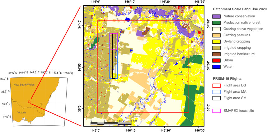
Figure 1. Location of the Yanco study region in southeastern Australia, with the areas captured by the various flights represented in different colors. The land use map in the background is based on the 50 m CLUM data (ABARES, 2021).

2.2 Datasets airborne campaign

2.2.1 Instruments on the aircraft

During the campaign, the aircraft carried a payload with multiple scientific instruments (Wu et al., 2019). Here, only the instruments used in this study are described. The Polarimetric K-band Scanning Radiometer (PKSR) was used for the Ka-band measurements. It is a horn-shaped radiometer with a center frequency of 36.5 GHz ($\lambda$ = 0.008 m) and a bandwidth of 1.8 GHz. It measured the brightness temperatures in both vertical (V) and horizontal (H) polarizations, with a 3 dB width of 3.9°. The Polarimetric L-band Multibeam Radiometer (PLMR) was also used in this study and measured brightness temperatures in both V and H polarizations at a center frequency of 1.413 GHz ($\lambda$ = 0.212 m) with a bandwidth of 24 MHz. The PLMR used a single receiver and measured at approximate incidence angles of 7°, 21.5°, and 38.5°. Warm and sky calibration were conducted for both the PLMR and PKSR before and after the flights, and water calibration was performed over Lake Wyangan during each flight.

2.2.2 Flights

Multiple flight strategies with various purposes were executed during the PRISM-19 campaign. For this study, three strategies were utilized. The first strategy, referred to as DS (Down Scaling) according to the original workplan (Wu et al., 2019), provided multi-angle observations of the Ka-band from the PKSR over the entire 40 km × 40 km region. The flights were conducted at an altitude of approximately 3,100 m (ASL), resulting in 3 dB footprints ranging from 200 to 400 m. For this study, the L-band PLMR observations from these DS flights were also utilized. These observations had larger footprints, ranging from 700 to 1,600 m. Five DS flights were included in this study to isolate and analyze the vegetation information from the Ka-band observations.

The second strategy, called SM (Soil Moisture) consisted of seven useful flights. These flights employed a fixed incidence angle of 15° and were conducted at a very low altitude of 300 m (ASL), resulting in 3 dB footprints ranging from 10 to 14 m. The SM flights were performed early in the morning to align with the overpass time of the Soil Moisture Active Passive (SMAP) satellite mission.

The third strategy used in this study was called MA (Multi-Angle). Although its name suggests otherwise, the Ka-band observations were taken at a fixed angle of 21°. The 7 MA flights took place on the same days as the SM flights but occurred later in the day. These flights were operated at a slightly higher altitude of approximately 430 m (ASL), resulting in 3 dB footprints of 20–24 m. Both the SM and MA flights were used in the LST analysis.

Table 1 provides a summary of all the flights used in this study and more details of this flight campaign can be found in Wu et al. (2019).

Table 1

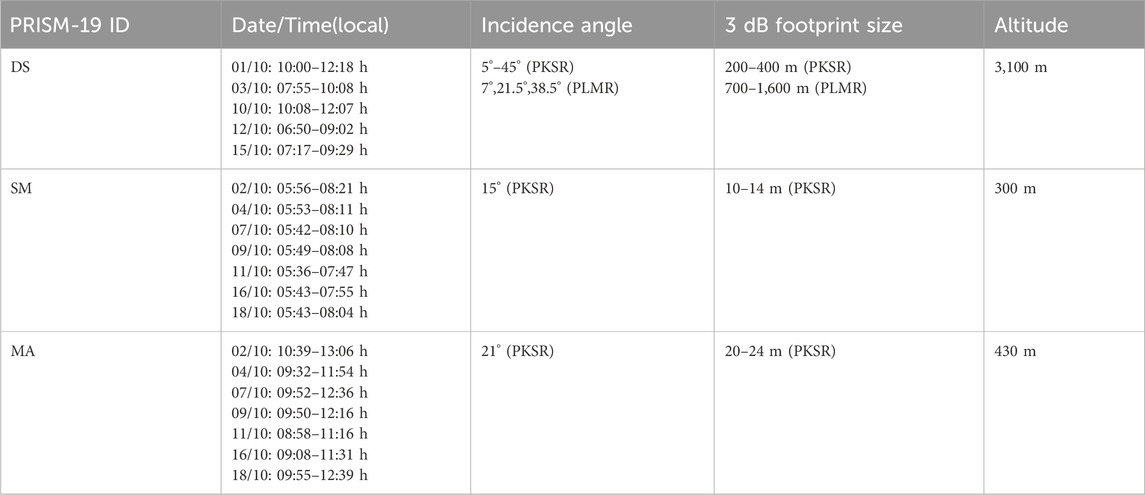
Table 1. Summary of the flights used in this study. The same flight IDs as described in Wu et al. (2019) are used, and the location of these flights is shown in Figure 1.

2.2.3 Ground sampling

Surface soil moisture sampling was measured at a depth of 0–5 cm was done using the Hydroprobe Data Acquisition System (HDAS) (Merlin et al., 2007). Measurements were taken across multiple agricultural fields at 50 m spacing over a 3-week period between 29 September and 18 October 2019. Ancillary information, including irrigation and vegetation type was collected alongside the soil moisture measurements. The soil moisture data was used in this study to analyze the sensitivity of the PKSR Ka-band observations to variations in moisture under different types of vegetation cover.

2.3 Satellite datasets

2.3.1 AMSR2

AMSR2 Level 3 (v.2.2, standard product) 0.25-degree gridded vertically and horizontally polarized brightness temperatures (Maeda et al., 2016) were collected for the study region, centered at 34.8528°S, 146.2276°E. The instrument is a conical scanning passive microwave radiometer onboard the Global Change Observation Mission–Water (GCOM-W) satellite platform of the Japan Aerospace Exploration Agency (JAXA). The satellite operates at an altitude of 700 km, with an ascending equator crossing time of 1:30 p.m. and a descending time of 1:30 a.m. Both the ascending and the descending observations of the 36.5 GHz channel were used. This frequency has a bandwidth of 1,000 MHz, a 3 dB ground resolution of 7 km × 12 km, and a radiometric resolution and sensitivity (i.e., Noise Equivalent delta Temperature NEdT) of 0.6 K. The instrument has an incidence angle of approximately 55°. Data for the period from July 2012 to October 2024 were obtained from the JAXA data portal (JAXA, 2024).

2.3.2 MODIS

Vegetation, LST and atmosphere products from the Moderate Resolution Imaging Spectroradiometer (MODIS) instrument on the Aqua spacecraft were used as reference data in this study. Daily day and night 1 km LST (MYD11A1 v6.1), 250 m NDVI (MYD13Q1 v6.1), and 1 km 16-day NDVI (MYD13A2 v6.1) products were obtained from the Application for Extracting and Exploring Analysis Ready Samples (AppEEARS, 2024) using the boundaries of the study region. Daily 1° total column precipitable water vapor (MYD08_D3 v6.1) and daily mean liquid cloud water (MYD08_D3 v6.1) were collected from the Earth Observing System Data and Information System (EOSDIS, 2024) for the period spanning July 2012 to October 2024.

2.3.3 Landsat

Two Landsat 8 images were used in this study. The Landsat scenes of October 2 and 18 October 2019, with path 93 and row 84, were selected. The overpass time of these images was approximately 10:08 a.m. local time. NDVI was calculated from the Level 2 surface reflectance estimates of the red band (Band 4) and the near-infrared band (Band 5), with a spatial resolution of 30 m. LST was derived from the thermal infrared Band 10, which has a resolution of 100 m. These two Landsat scenes only cover the area of the SM and MA flights. All data was obtained from the Earth Explorer data portal (Earth Explorer, 2024).

2.3.4 Satellite derived VOD and soil moisture

Moreover, VOD products were obtained from the VOD Climate Archive v2 (VODCA v2) dataset (Zotta et al., 2024a). Data for the study region, centered at 34.8528°S, 146.2276°E were collected. The data were available at a daily temporal resolution and a spatial resolution of 0.25°. Single frequency VOD data was extracted from this data set and made available for this study. AMSR2-based VOD data from C-, X-, and Ku-band were extracted for the period from July 2012 to December 2021. For L-band, the SMAP-based VOD data was extracted from the same dataset. For this frequency data were obtained for the period from April 2015 to December 2021. VOD was derived using the Land Parameter Retrieval Model (Owe et al., 2008; van der Schalie et al., 2017). Data from VODCA v2 are freely accessible and described in detail by Zotta et al. (2024b).

Soil moisture time series from the same period were extracted from the European Space Agency Climate Change Initiative Soil Moisture (ESA CCI SM) data record (Dorigo et al., 2017; Gruber et al., 2019). ESA CCI SM (v08.1) was downloaded from the Comprehensive Environmental Data Archive (CEDA, 2024) and for this study, only the passive microwave retrievals from SMAP at 0.25° resolution were used.

3 Methods

Passive microwave Ka-band observations over land, as derived from the satellite and airborne platform, were investigated. Various statistical techniques were applied and a radiative transfer model was used for the extraction of the vegetation signal from the original Ka-band observations. In the following sections, both the model and the statistical analysis are described.

3.1 Radiative transfer model for Ka-band

The brightness temperatures measured by microwave radiometers can be simulated by radiative transfer models. Here, the updated model for Ka-band prediction introduced by Holmes et al. (2009) was used, which is based on a commonly used description of microwave emission of vegetation cover (Mo et al., 1982). Accordingly, the brightness temperature as measured at the satellite can be described by

$T_{B,P}=T_{B,extra}+T_{B,P,au}+{\mathrm{\Gamma }}_a\left[{\mathrm{\Gamma }}_v\left(1-R_{rs,P}\right)T_S+\left(1-{\mathrm{\Gamma }}_v\right)\left(1-\omega \right)T_v+\left(1-{\mathrm{\Gamma }}_v\right)\left(1-\omega \right)T_v{R}_{rs,P}{\mathrm{\Gamma }}_v+T_{B,P,ad}{R}_{rs,P}{\mathrm{\Gamma }}_v^2\right](1)$

where $T_{B,extra}$ is the extraterrestrial background cosmic radiation. This is estimated to be 2.7 K and is independent of frequency and incidence angle (Ulaby et al., 1981). $T_{B,P,au}$ and $T_{B,P,ad}$ are the upward and downward atmospheric brightness temperature at polarization P ([V] or [H]) and ${\mathrm{\Gamma }}_a$ is the atmospheric transmissivity. ${\mathrm{\Gamma }}_v$ is the vegetation transmissivity, $\omega$ is the single scattering albedo of the vegetation and $R_{rs,P}$ the rough surface reflectivity. The rough surface reflectivity ($\left.R_{rs,P}\right)$ is equal to 1 minus the rough surface emissivity ($e_{rs,P}$). $T_S$ is the soil temperature and $T_v$ the vegetation canopy temperature, both in Kelvin.

The rough surface reflectivity can be derived from the Fresnel relationships in combination with a roughness model. Fresnel describes the smooth surface reflectivity ($R_{ss,P}$), as a function of the dielectric constant of the soil. The dielectric constant of the soil is directly linked to soil moisture and can be modelled with a dielectric mixing model (e.g., Calvet et al., 1995; Park et al., 2019; Wang and Schmugge, 1980). The rough surface reflectivity ($R_{rs,P}$) can be calculated from the smooth surface reflectivity ($R_{ss,P}$), by correcting for the effect of roughness using the Q parameter for cross polarization and h for the roughness height (Wang and Choudhury, 1981) according to

$R_{rs,\left[V\right]}=\left(Q{R}_{ss,\left[H\right]}+\left(1-Q\right)R_{ss,\left[V\right]}\right){\mathit{exp}}^{-h\cos \left(u\right)}(2)$

$R_{rs,\left[H\right]}=\left(Q{R}_{ss,\left[V\right]}+\left(1-Q\right)R_{ss,\left[H\right]}\right){\mathit{exp}}^{-h\cos \left(u\right)}(3)$

where u is the incidence angle.

The atmospheric transmissivity is a function of the zenith atmospheric opacity (${\tau }_a$) and incidence angle ($u$) and can be described by

${\mathrm{\Gamma }}_a={\mathit{exp}}^{-{\tau }_a\sec \left(u\right)}(4)$

The atmospheric opacity ${\tau }_a$ is a function of atmospheric water content and can be estimated using the approximation of Choudhury et al. (1992) where the ${\tau }_a$ of Ka-band was described as a function of precipitable water (V) and cloud liquid water content (L) in mm according to

${\tau }_a=0.030+0.0022V+0.155L(5)$

Moreover, $T_{B,P,au}$ is a function of the effective air temperature ($T_e$) and ${\mathrm{\Gamma }}_a$ according to

$T_{B,P,au}=T_e\left(1-{\mathrm{\Gamma }}_a\right)(6)$

while $T_{B,P,ad}$ is equal to the sum of $T_{B,P,au}$ and the cosmic background radiation $T_{B,extra}$. The vegetation transmissivity is a function of VOD (${\tau }_v$) and the incidence angle (u) such that

${\mathrm{\Gamma }}_v={\mathit{exp}}^{-{\tau }_v\sec \left(u\right)}(7)$

The VOD (${\tau }_v$) can be derived using the analytical solution of Meesters et al. (2005) as

${\tau }_v=\cos \left(u\right)\ln \left(ad+\sqrt{{\left(ad\right)}^2+a+1}\right)(8)$

where

$a=\frac{1}{2}\left[\frac{\left(e_{rs,\left[V\right]}-e_{rs,\left[H\right]}\right)}{MPDI}-e_{rs,\left[V\right]}-e_{rs,\left[H\right]}\right](9)$

and

$d=\frac{1}{2}\frac{\omega }{\left(1-\omega \right)}(10)$

The Microwave Polarization Difference Index (MPDI) is defined as

$MPDI=\frac{T_{B,\left[V\right]}-T_{B,\left[H\right]}}{T_{B,\left[V\right]}+T_{B,\left[H\right]}}(11)$

The VOD (${\tau }_v$) is presented in numerous studies and Frappart et al. (2020) provides a review of this complex parameter. It is determined by the dielectric properties of the vegetation layer as well as by the vegetation architecture (e.g., density, structure and orientation) (Grant et al., 2016). When describing the VOD as a measurement of attenuation of radiation by the vegetation it can be expressed as

${\tau }_v=H_v\left(\frac{4\pi }{\lambda }\sqrt{{ℇ}_v^{″}}\right)\frac{1}{1-\omega }(12)$

where is $H_v$ is the height of the vegetation layer in m, $\lambda$ the wavelength in m, and ${ℇ}_v^{″}$ the imaginary part of the dielectric constant of the vegetation layer. The dielectric constant of the vegetation is strongly related to the vegetation water content.

For observations close to the Earth surface (i.e., ground observations, or observations from an aircraft) the microwave signal does not have to cross the entire atmosphere. Therefore, for the aircraft observations, Equation 1 can be simplified to

$T_{B,P}={\mathrm{\Gamma }}_v\left(1-R_{rs,P}\right)T_S+\left(1-{\mathrm{\Gamma }}_v\right)\left(1-\omega \right)T_v+\left(1-{\mathrm{\Gamma }}_v\right)\left(1-\omega \right)T_v{R}_{rs,P}{\mathrm{\Gamma }}_v+T_{B,P,ad}{R}_{rs,P}{\mathrm{\Gamma }}_v^2(13)$

3.2 Statistical analysis

The Ka-band satellite and aircraft data were analyzed to reveal their sensitivity to temperature and vegetation at different scales. First, the vertically polarized Ka-band satellite brightness temperatures were compared to MODIS LST to better understand their relationship for the study region. Regression analyses were applied to quantify this relationship, and the influence of vegetation and moisture was investigated using MODIS NDVI and SMAP soil moisture. A similar analysis was then conducted on the aircraft data, using LST and vegetation (NDVI) data from Landsat, and ground observations of soil moisture from HDAS. Only the SM and MA flights were used because these flights produced the highest spatial resolution and had similar overpass times to Landsat and the ground observations. By using this two-step approach, the similarities and differences in sensitivity between the Ka-band observations from the aircraft and those from the satellite were demonstrated.

Second, the VOD was calculated using a radiative transfer model for Ka-band as described in the previous section using Equation 1 – 13. The VOD was calculated for both the satellite and aircraft data to isolate the vegetation signal. The Ka-band VOD at satellite scale was compared to VOD satellite products from other frequencies, including L-, C-, X-, and Ku-band. These single frequency VOD products were extracted from the VODCA v2 dataset. In addition, NDVI maps from MODIS were also included in this comparison analysis and regression analyses were applied to obtain the relationship between the different data products.

The aircraft Ka-band VOD was derived from the observations with an incidence angle between 35° and 45° degrees and compared to MODIS NDVI maps. Here, only the observations from the DS flights were used, as these flights provided observations at angles greater than 35°. These wider angles impose a constraint on providing a realistic VOD derivation using the analytical solution of Meesters et al. (2005), as described in Equations 8–11. In addition, the aircraft Ka-band observatons were also compared to L-band aircraft observations (PLMR) to assess the change in vegetation sensitivity across frequencies. These statistical analyses allow for a better assessment into the usability of the Ka-band observations for land monitoring applications at different scales.

4 Results

4.1 Land surface temperature (LST)

4.1.1 Satellite observations

The Ka-band vertically polarized brightness temperatures as measured by the AMSR2 satellite instrument were compared to the daily LST data from MODIS for the Yanco study region for the period from July 2012 to October 2024. Both instruments were on the same platform (Aqua), which made it possible to provide collocated measurements on both the ascending (day) and descending (night) nodes. A regression analysis with these two categorical covariates was applied. This resulted in an R² of 0.98, for 3,175 observations with a Root Mean Square Error (RMSE) of 2.1 K. The Standard Error of the estimated LST (SE) is 2.2 K for the ascending and 2.1 K for the descending observations.

Figure 2 provides a graphical presentation of this relationship. A regression analysis with categorical covariates was also applied to variations in vegetation and moisture using MODIS NDVI and SMAP soil moisture, respectively (not shown). The average soil moisture value of SMAP was 0.19 m³ m⁻³ with a standard deviation of 0.10 m³ m⁻³ for this region. The average MODIS NDVI was 0.43 with a standard deviation of 0.14. Despite the variability in both soil moisture and vegetation, none of these combinations resulted in a p-value <0.05 indicating that these categories were not able to significantly differentiate the linear relationship between LST and the vertically polarized Ka-band observations.

Figure 2

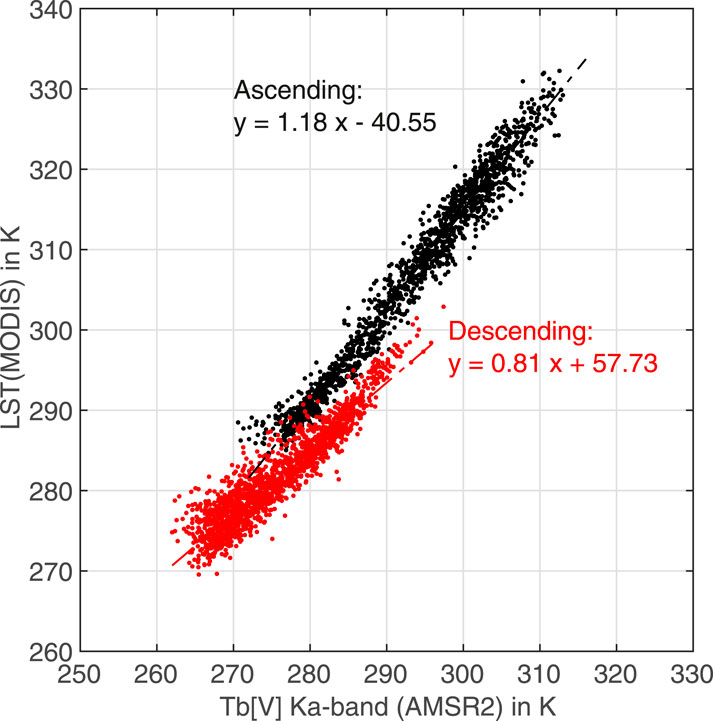
Figure 2. Comparison between vertically polarized Ka-band observations from AMSR2 and MODIS LST for the ascending (day) and descending (night) observations.

4.1.2 Aircraft observations

In Figures 3, 4, the vertically polarized brightness temperatures measured by the PKSR were mapped for each individual flight. Figure 3 presents the high-resolution SM flights conducted early in the morning, while Figure 4 depicts the MA flights. For visualization purposes the individual 3 dB footprints were enlarged by a factor of 5 (i.e., to 75 m) for the SM flights, and a factor of 3 (i.e., to 75 m) for the MA flights. The images are cut-outs of the SMAPEX site as shown in Figure 2.

Figure 3

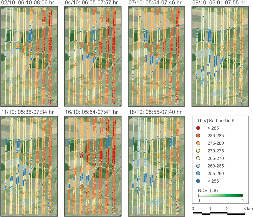
Figure 3. An overview of the Ka-band PKSR observations during the SM flights used in this study. The footprint size is increased by a factor of five (i.e., to 75 m) for visualization purposes, with the background being a Landsat 8 NDVI image from 18 October 2019.

Figure 4

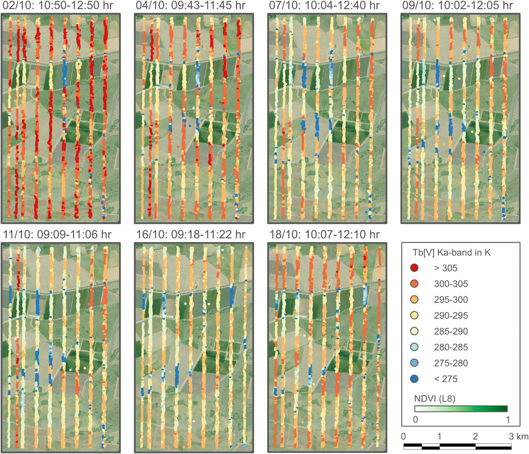
Figure 4. An overview of the Ka-band PKSR observations during the MA flights used in this study. The footprint size is increased by a factor of 3 (i.e., to 75 m) for visualization purposes, with the background being a Landsat 8 NDVI image from 18 October 2019.

Both figures show consistent spatial clusters, with low brightness temperature values over agricultural/vegetated sites and higher values over sparsely vegetated regions. In Figure 3, a clear temperature trend is observed from west to east, corresponding to a LST increase during the flight as the day progressed. This trend is less pronounced in the MA flights, where the warming gradient is much smaller as compared to the early morning flights. Additionally, low brightness temperature values are observed in the southwestern part of both the SM and MA flights over the bare agricultural fields. These low values start to appear around October 4 and become more evident from October 9 onwards, likely due to irrigation events in these areas.

The vertically polarized Ka-band observations from the MA flights on October 2 and October 18 are selected and compared to LST and NDVI from Landsat 8. The Ka-band observations were detrended over time to account for the temperature increase during the flight. Only stable observations (i.e., those recorded at a flight altitude between 420 and 440 m) were included, and the data were limited to a 1.5-h time frame relative to the Landsat overpass. Observations over water bodies and drainage canals were excluded from the analysis.

Figure 5 presents four scatterplots that clearly illustrate the impact of vegetation on the spatial temperature pattens. For four NDVI bins (i.e., < 0.2, 0.2–0.4, 0.4–0.6 and ≥0.6) the relationship between Ka-band and LST was plotted. For the low NDVI values (up to 0.6) the scatter is high with low R² values ranging from 0.24 to 0.43 as shown in Figures 5A–C. Within this NDVI range the vertically polarized Ka-band observations appeared to be more sensitive to surface and soil characteristics. However, with higher NDVI values the Pearson correlation increases, reaching an R² of 0.7 for locations with Landsat NDVI ≥0.6 as illustrated in Figure 5D. Table 2 provides the details of this analysis including the evaluation metrics of the individual days and the metrics where both days are used.

Figure 5

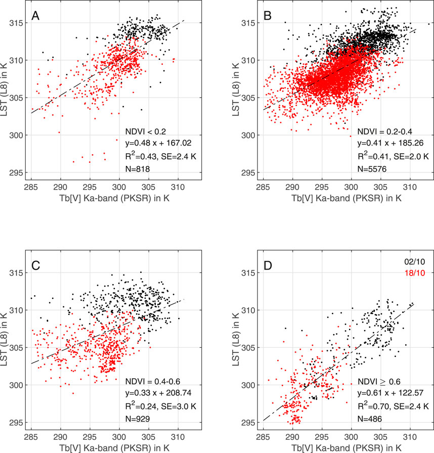
Figure 5. Four scatterplots of the aircraft vertically polarized Ka-band observations from PKSR and LST from two Landsat 8 (L8) images. The black dots represent the image of 2 October and the red dots the image of 18 October. In plot (A) all data where Landsat NDVI <0.2 are plotted, (B) only datapoints where NDVI is between 0.2 and 0.4, (C) where NDVI is between 0.4 and 0.6 and (D) where NDVI ≥0.6. The statistics of this analysis are summarized in Table 2.

Table 2

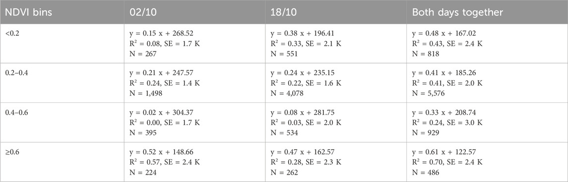
Table 2. Summary of the linear regression analysis between vertical polarized Ka-band observations from the MA flights and LST from Landsat 8 for four different NDVI bins.

The Ka-band vertically polarized brightness temperatures were also compared to soil moisture. Observations from SM flights were used for this analysis due to their high spatial resolution and their overpass time being close to the in situ soil moisture measurements. Soil moisture was measured at 50 m intervals, so only data pairs with a maximum distance of 25 m between the soil moisture measurements and the aircraft observations were selected. Furthermore, only observations within a 2-h time frame of the aircraft overpass were included, based on the assumption that soil moisture changes were negligible within this period.

It was assumed that the Landsat NDVI image from October 2 was representative of the flights conducted on October 2, 4, 7, and 9, while the Landsat NDVI image from October 18 was considered representative of the flights on October 11, 16 and 18. Data pairs were divided into two groups based on the NDVI values: one group with NDVI <0.6 and another with NDVI ≥0.6. The brightness temperatures were plotted against the measured soil moisture (Figure 6).

Figure 6

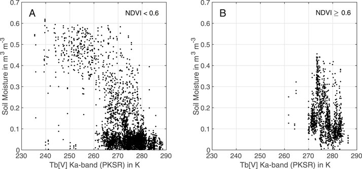
Figure 6. Scatter plot comparing the vertically polarized Ka-band observations of PKSR with ground measurements of soil moisture. Two subsets are displayed. (A) scatterplot where only data with Landsat 8 NDVI values <0.6 are selected and (B) scatterplot where only Landsat 8 NDVI values ≥0.6 are selected.

The results indicate that when NDVI values were high, the vertically polarized brightness temperatures showed limited sensitivity to soil moisture. Conversely, when NDVI values were low, the brightness temperatures exhibited a stronger sensitivity to soil moisture. Particularly wet soils (soil moisture >0.3 m³ m⁻³) can cause a reduction in brightness temperatures of approximately 20 K.

4.2 Vegetation optical depth (VOD)

4.2.1 Satellite observations

The VOD for the AMSR2 Ka-band satellite observations was calculated using the radiative transfer model described in Section 3.1. Only the descending (nighttime) observations were used to align with the available VODCA v2 products, which are soley based on descending observations (Zotta et al., 2024b). Soil temperature (T_s) was estimated from vertically polarized Ka-band brightness temperatures using the equation for descending observations as provided in Figure 2 in Section 4.1. At this time of day, the vegetation canopy temperature (T_v) was assumed to be equal to the soil temperature. The atmospheric opacity (${\tau }_a$) was parameterized using the MODIS precipitable water vapor and liquid cloud water products, resulting in an average opacity of 0.075 +/− 0.020. The effective air temperature (T_e) was calculated as a direct function of T_s, based on the formulation of Bevis et al. (1992). A surface roughness height (h) of 0.1, a cross-polarization parameter (Q) of 0.1 and a single scattering albedo ($\omega$) of 0.03 were used. These three parameters were iteratively derived to achieve full convergence between the simulated and observed brightness temperatures. The Ka-band VOD was subsequently calculated using Equation 8 based on Meesters et al. (2005). Table 3 provides a summary of these different input parameters.

Table 3

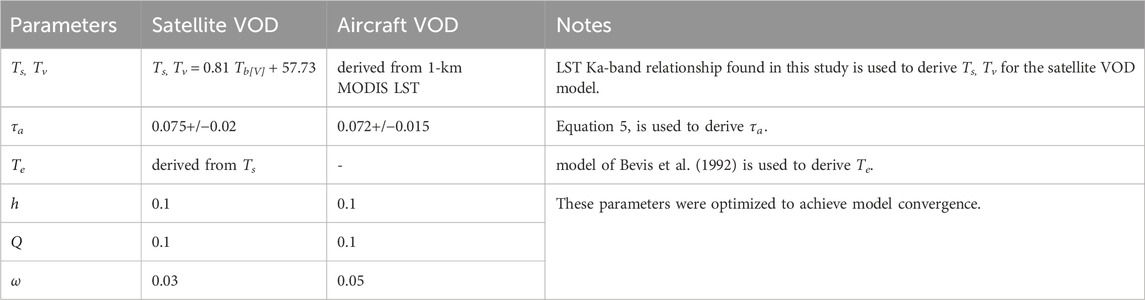
Table 3. Input parameters for the radiative transfer model used to derive VOD.

The derived AMSR2 VOD was compared to the VODCA v2 products (Zotta et al., 2024b) at various frequencies based on AMSR2 and SMAP. The results of this comparison are presented in Figure 7. The Ka-band VOD exhibits a strong linear relationship with the Ku-, X- and C-band VOD with an R² decreasing from 0.79 to 0.69 as the frequency decreases. The L-band VOD, derived from the SMAP satellite, showed a poor correlation with the Ka-band VOD, with an R² of only 0.14. The range of VOD at Ka-band was approximately between 0.4 and 1.3. This range, as well as the absolute VOD values, decreased for lower frequencies. For Ku-band, the range is between 0.2 and 0.9, while at L-band, the range narrowed further to between 0 and 0.2.

Figure 7

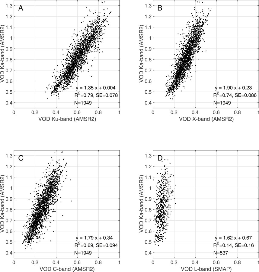
Figure 7. Four scatterplots showing the relationship of AMSR2 Ka-band VOD with the other frequencies. The Ka-band VOD is compared to (A) AMSR2 Ku-band, (B) AMSR2 X-band, (C) AMSR2 C-band and (D) SMAP L-band from the VODCA v2 dataset.

A time series of the VOD products is presented in Figure 8, alongside the NDVI time series for comparison. The 1 km, 16-day NDVI data from MODIS were averaged over the study region to align with the spatial resolution of the VOD data. The AMSR-2 based VODs span a period over 12 years (2012–2024), while the L-band VOD from SMAP begins in 2015 corresponding to the satellite’s launch. The time-series revealed strong seasonal and interannual variability in both VOD and NDVI. The Ka-, Ku-, X-, and C- band VOD demonstrated strong temporal similarities and matched well with NDVI variability. However, the L-band VOD appeared noisier and less responsive to vegetation variations, as it is more sensitive to non-green tissues like branches and trunks (Frappart et al., 2020).

Figure 8

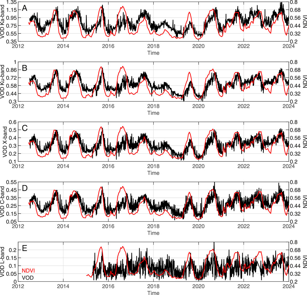
Figure 8. Time series of the satellite derived VOD (black) and MODIS NDVI (red). (A) AMSR2 Ka-VOD, (B) AMSR2 Ku-band VOD, (C) AMSR2 X-band VOD, (D) AMSR2 C-band VOD, and (E) SMAP L-band VOD. The VOD time series as presented in (A) was derived in this study. The VODs in (B–E) are from the VODCA v2 dataset.

Despite the strong similarities, small phase shifts in seasonality between the NDVI and VOD were observed. These shifts have been found in multiple studies (e.g., Jones et al., 2012; Andela et al., 2013; Grant et al., 2016) and reflects the biophysical differences in the phenology parameters measured by the two different vegetation proxies (Jones et al., 2011). The NDVI is synergistic with vegetation greenness, whereas VOD is more related to vegetation water content and biomass. Therefore, both may follow a different seasonal cycle depending on vegetation type and weather conditions.

Figure 9 compares all VODs to NDVI, with both Pearson (R2) and Spearman rank (R2s) correlation coefficients to account for potential non-linear relationships. The Ka- and Ku-band VOD yield similar statistics with R2svalues of 0.52 and 0.53, and R2 values of 0.45 and 0.46, respectively (Figures 9A,B). The highest correlations were observed for the X- and C-band VOD, with R2s values of 0.58 and 0.57, respectively (Figures 9C,D). For NDVI values above 0.4, the spread in data points increased, and maximum VOD values appeared to saturate. At L-band, the correlation between VOD and NDVI was weak, with an R2 value of 0.1 and a R2s value of 0.14 (Figure 9E). At this frequency, the spread in data points remained consistent across the entire NDVI range.

Figure 9

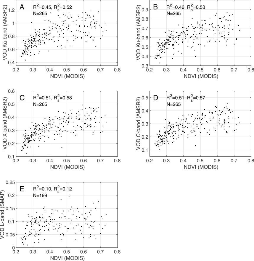
Figure 9. Scatterplots comparing the satellite derived VODs with NDVI. (A) Ka-band VOD, (B) Ku-band, (C) X-band VOD, (D) C-band VOD, and (E) L-band VOD. The VOD data as presented in (A) were derived in this study. The VODs in (B–E) are from the VODCA v2 dataset. The correlation coefficients are based on Pearson (R²) and Spearman rank (${\mathit{R}}_{\mathit{s}}^{\mathbf{2}}$) correlations.

4.2.2 Aircraft observations

The VOD derivation method as proposed by Meesters et al. (2005) and applied in this study to estimate the Ka-band VOD for AMSR2 uses the MPDI as a tool to isolate the microwave vegetation signal. The size and range of the MPDI are influenced by the incidence angle. Figure 10 illustrates this effect, showing MPDI observations from the PKSR plotted against the incidence angle during their high-altitude DS flights. At angles below 20° the difference between horizontally polarized and vertically polarized brightness temperature is minimal, making it challenging to differentiate the vegetation signal. With an increasing angle the range in MPDI increased up to 0.03 for the highest angles.

Figure 10

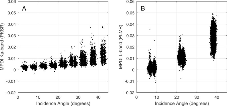
Figure 10. The incidence angle compared to the MPDI for (A) the PKSR Ka-band observations and (B) the PLMR L-band observations. For this plot the observations of the DS flight of 3 October 2019 were used. Plots of the other four flights provided similar results.

For comparison, this relationship is also presented for airborne L-band observations from the PLMR. Although only three angle bins were used for L-band data, the results show a significantly larger MPDI range at higher angles, with values increasing up to 0.01–0.05 for the largest angle bins. Notably, the MPDI range at L-band was approximately twice as large as that at Ka-band. In addition, the lowest MPDI values at the highest angle bins were approximately 0.01 at L-band. At Ka-band these values were lower at around 0.004.

When cross-comparing both plots (i.e., Figures 10A, B), the range in MPDI values for incidence angles below 10° seems to be substantially smaller for Ka-band (Standard Deviation (SD) MPDI = 8.23 × 10⁻⁴ for 0°–5°, and SD MPDI = 8.59 × 10⁻⁴ for 5°–10°), whereas for L-band (SD MPDI = 2.06 × 10⁻³ for 5°–10°). At these low angles, the brightness temperatures of the two different polarizations should behave similarly; therefore, the demonstrated MPDI range could be associated with the capabilities of each microwave instrument. This suggests a higher sensitivity in measuring MPDI with the Ka-band sensor compared to that of L-band. Conversely, the range at L-band is larger for the higher angles (>35°), primarily due to its increased sensitivity to soil moisture resulting from lower vegetation attenuation. Consequently, both instrumental uncertainty in measuring MPDI and the characteristics of the given frequency define how well the vegetation dynamics can be measured.

The airborne MPDI values were also plotted against the NDVI to analyze their relationship. The 250 m 16-day NDVI MODIS data was used, as it matched the spatial resolution of the PKSR observations during the DS flights and provided complete coverage of the flight area. Landsat 8 scenes, which were used in prior analysis, were unsuitable here due to limited coverage of the DS flight areas. Figure 11 presents three scatter density plots, selecting only MPDI values with incidence angles between 35° and 40° for the PKSR and PLMR measurements. In Figures 11A, B, the MPDI values for the Ka-band and L-band, respectively, were plotted against the average MODIS NDVI values derived from data from September 30 and October 16. Both bands showed a negative correlation with NDVI, having R² = 0.21 (R = −0.46) and $R_s^2$ = 0.26 for Ka-band (N = 3,470), while having R² = 0.33 (R = −0.57) and $R_s^2$ = 0.32 for L-band (N = 40,958). All correlations were statistically significant (p-value <0.05), though the correlation strength was relatively low. The L-band demonstrated a broader range at higher NDVI values, suggesting reduced saturation for denser vegetation cover compared to the Ka-band. Notably, the spread in data points was high for both bands. Figure 11C compares the MPDI values of the Ka-band (PKSR) with those of the L-band (PLMR). Data pairs were selected based on a maximum distance of 100 m between the footprint centers of the two observations, resulting in 1925 data points. The scatter plot indicates a positive correlation between the two bands, albeit weak, with R² = 0.30 and $R_s^2$ = 0.32. The correlation is statistically significant (p-value <0.05), suggesting some degree of consistency between the two bands despite the differences in frequency and observation characteristics.

Figure 11

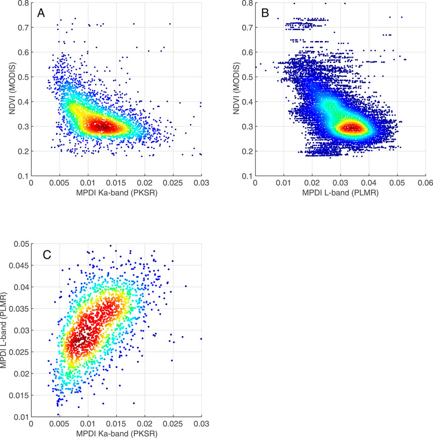
Figure 11. Scatter density plots of MPDI observations from the DS flights at incidence angles between 35° and 40°. (A) MPDI of Ka-band (PKSR) versus NDVI (MODIS), (B) MPDI of L-band (PLMR) versus the NDVI (MODIS), and (C) Ka-band MPDI(PKSR) compared to the L-band (PLMR). The color scale represents the probability density, where dark blue indicates the lowest and dark red represents the highest probability density estimation.

The VOD for the airborne Ka-band (PKSR) observations from the DS flights was calculated for incidence angles between 35° and 45° using the radiative transfer model as described in Equation 13. This equation considers the lower observation altitude of the aircraft as compared to the satellite, resulting in a smaller atmospheric contribution. Unfortunately, the soil temperature (T_s) could not be derived from the vertically polarized Ka-band brightness temperatures from the PKSR due to its sensitivity to variations in surface characteristics, as demonstrated in Section 4.1.2. Therefore, the daily 1-km MODIS LST was used as an alternative approximation for both the soil (T_s) and the vegetation canopy temperature (T_v). MODIS LST had different overpass times compared to the flights, which could easily result in incorrect temperature estimation. To mitigate this issue of time differences, only flights with a similar morning overpass were selected. In addition, only days when MODIS LST was not hindered by clouds were used. This selection criterion resulted in two flights that were eligible for the VOD calculation: the DS flights of 3 October and 15 October.

The Ka-band observations were detrended over time to account for the temperature increase during the flight. Using the atmospheric data of MODIS, the atmospheric opacity (${\tau }_a$) was estimated to be 0.072 +/− 0.015. The surface roughness height (h), and cross-polarization parameter (Q) were assumed to have the same value as those at the satellite scale (both 0.1), and a single scattering albedo ($\omega$) of 0.05 was iteratively derived to achieve model convergence. Table 3 provides a summary of these input parameters. The derived Ka-band VOD from the PKSR had a comparable range as the satellite VOD and ranged from approximately 0.3–1. The VOD estimates are presented in Figure 12. The VOD values of both days were plotted in one map to achieve a better coverage. Despite the noisy spatial VOD signal, some consistent spatial clusters were observable. In general, high values (>0.8) were found over the agricultural/vegetated sites and low values (<0.4) over the more sparsely vegetated regions.

Figure 12

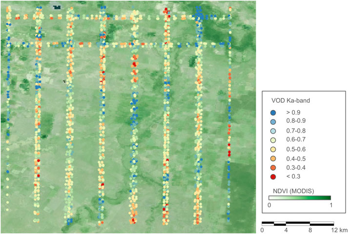
Figure 12. Ka-band VOD from the PKSR as derived from two DS flights on October 3 and October 15 using observations with incidence angles between 35° and 45°. The point size was set to 400 m to approximate the actual 3 dB footprint size. The background is a 250-m MODIS NDVI image of this period.

In Figure 13A, the VOD is compared to the MODIS NDVI. The VOD of October 3 was connected to the MODIS NDVI of September 30, and the VOD of October 15 was connected to the MODIS NDVI of October 15. The data are scattered and exhibit a low correlation (R² = 0.12, p-value<0.05), although the pattern revealed a similar increasing trend as observed in the satellite data (see Figure 9A). In Figure 13B the VOD was compared to L-band MPDI from the PLMR. To be consistent with the L-band MPDI of PLMR, only the Ka-band VOD derivatives from 35° to 40° angles were plotted. Despite the weak correlation, the negative trend was significant (R² = 0.27, p-value <0.05).

Figure 13

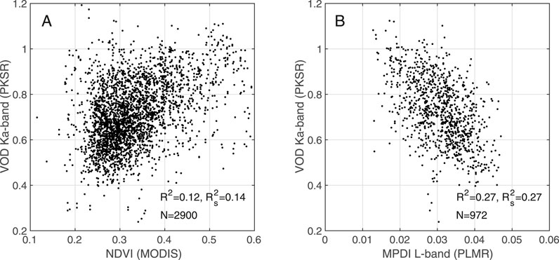
Figure 13. (A) aircraft derived Ka-band VOD compared to MODIS NDVI, and (B) aircraft derived Ka-band VOD compared to L-band MPDI.

5 Discussion

5.1 LST and VOD derivation at different spatial scales

The vertically polarized brightness temperatures at the Ka-band frequency have been used as a key input for various LST retrieval approaches (e.g., Holmes et al., 2009; Prigent et al., 2016). In this study, sensitivity to temperature has been confirmed for the Yanco study region. It was possible to derive LST using AMSR2 satellite observations through a simple linear relationship with a high degree of accuracy (R² = 0.98, RMSE = 2.1 K as compared to MODIS LST). In other studies, the RMSE for Ka-band based LST retrievals varied between 2 and 5 K (Duan et al., 2020), illustrating that this retrieval can be considered a high-quality retrieval. This is probably due to the relatively stable surface emissivity at this frequency over this region at satellite scale. The atmospheric opacity is relatively low (average ${\tau }_a$ = 0.075 +/− 0.020), and the vegetation cover is dense enough (average Ka-band VOD = 0.82 +/− 0.17) for this frequency to attenuate the influence of soil moisture. With the PKSR Ka-band observations from the PRISM-19 campaign, it was also possible to conduct a spatial analysis of the vertically polarized brightness temperature with a much higher resolution up to 10 m. Here, a strong linear relationship was also found, but only for regions with sufficient vegetation cover. The aircraft retrievals were obtained from observations with low fixed angles of 15° and 21°, respectively, whereas the satellite-derived LST used Ka-band observations with an angle of 55°. They all showed a strong correlation with LST from MODIS and Landsat, illustrating the ability to derive LST from Ka-band observations at multiple angles.

A non-linear scaling relationship between the Ka-band observations and their ability to estimate LST was found. At the 7 km × 12 km satellite footprint of AMSR2, the influence of local variability in moisture and vegetation is dampened. For example, small irrigated agricultural fields of only a few hectares in size, with high moisture values and low vegetation cover, will most likely have a negligible contribution to the overall measured brightness temperatures because these fields cover less than 1% of the total footprint. However, for the aircraft observations with a resolution of approximately 12 m × 14 m, irrigated agricultural fields covered the entire footprint, making the impact visible with a significant drop in brightness temperature (up to 20 K). Similar behavior can be observed with VOD, where the VOD signal became much noisier and exhibited a weaker relationship with NDVI in the aircraft data compared to the satellite. Here, local vegetation scattering and the potential oversimplification of the radiative transfer model at the local scale could have played a role. For example, for both satellite and airborne VOD retrievals, the assumption was made that the soil temperature (T_s) is equal to the vegetation canopy temperature (T_v). While this might be true for the coarse scale descending (nighttime) satellite observations, it is less likely to be true for the high resolution aircraft flights. Xiao et al. (2024) addressed the impact of oversimplication on T_s and T_v estimates for VOD retrievals. They could increase uncertainty in VOD and therefore contribute to the higher noise levels in the aircraft Ka-band VOD. Scaling effects like these are generally well-known in remote sensing, and numerous studies have addressed these issues (e.g., Pu and Bonafoni, 2021; Peng et al., 2017; Sabaghy et al., 2020). For Ka-band, similar issues appeared because of the strong heterogeneous dynamics of moisture, temperature and vegetation and their influence on this frequency. Airborne campaigns like PRISM-19 make it possible to reveal some of these sensitivities that are not always visible at the satellite scale.

With the upcoming launch of the ESA mission CIMR, the Ka-band frequency will most likely be measuring at a targeted footprint size of approximately 3.3 km × 5.6 km (Donlon, 2023), which is 4.5 times sharper than AMSR2. With this new instrument, it will be possible to better detect and monitor large irrigated fields (>1 km²) at Ka-band, which are currently not visible to AMSR2. This will most likely be valid for the first part of the growing season when the vegetation cover is not yet too dense for this frequency to penetrate. Ka-band observations will not be able to provide accurate soil moisture values, but they should be able to detect changes when the fields are irrigated, as shown in this study with aircraft data.

5.2 The added value of Ka-band VOD

The satellite VOD was calculated for different frequencies. The retrieved Ka-band VOD showed strong similarities with the Ku-, X-, and C-band observations from the same AMSR2 instrument. The use of this frequency for vegetation monitoring, and in particularly for the derivation of VOD, has so far been overlooked. This study demonstrates that it is possible to derive realistic VOD values from this frequency. However, the Ka-band VOD was only calculated for one specific semi-arid region in Australia. It is not yet clear how well the Ka-band VOD retrievals will perform over other regions or land cover types, and so more research is needed to explore this. Nevertheless, having realistic Ka-band VOD from satellite observations could be an interesting addition to the already available VOD products. This frequency has a long legacy and radiometers with this frequency have been on numerous satellites (e.g., SMMR, AMSR, AMSR2, and the Special Scanning Microwave Imager (SSMI)). This makes it possible to analyze data records spanning multiple decades across diurnal variations. In the VODCA v2 dataset of Zotta et al. (2024b), C-, X- and Ku-band VOD were merged into one VOD product. Adding an additional Ka-band in their approach could potentially lead to a more robust VOD product.

The current available soil moisture algorithms for passive microwave data still struggle with the correction for vegetation. This correction is often performed in a simplified manner, which could lead to spurious vegetation-based signals in the soil moisture retrievals (Crow et al., 2025; Zwieback et al., 2019). This study demonstrated alignment between the different VODs, illustrating how vegetation affects the microwave signals in a similar way for the different frequencies. Using multiple frequencies instead of one single frequency is expected to support further improvement in the vegetation correction.

Ka-band VOD was also derived from aircraft observations. Although the VOD signal was still noisy it captured realistic patterns, with high values over the more densely vegetated parts of the study regions. Conducting a fully optimized model parameterization to retrieve the best Ka-band VOD was beyond the scope of this study, so improvements in this study framework can still be made. For example, a better estimation of vegetation and soil temperature during the flights would likely lead to a more robust VOD. In this study, the temperature was estimated using MODIS LST data, which was not collected at the exact same time as the PKSR observations. However, being able to derive VOD at a much higher spatial resolution could support validation, which is still considered a critical challenge (Feldman, 2024; Yao et al., 2024). Being able to derive realistic VOD values from aircraft or ground observations could create the opportunity to investigate its sensitivity to different vegetation characteristics at a much finer scale, which could further advance research on VOD.

5.3 Ka-band and L-band

Both the Ka-band and L-band observations from the aircraft showed some remarkable similarities, despite the difference in frequency and observation footprint. With data from the PKSR and PLMR, it was possible to cross-compare the two frequencies with similar angle bins. Here, the MPDI was used, being a direct microwave observation and considered as a powerful index to minimize the effect of soil and vegetation temperature (Owe et al., 2001). Moreover, both VOD and soil moisture can be linked to the MPDI (Meesters et al., 2005). The vegetation influences the microwave signal of the two frequencies in a similar way, but with different intensity. The vegetation attenuation at Ka-band was much stronger, resulting in a smaller MPDI range and faster saturation with low MPDI values close to zero. At L-band the vegetation saturation level had not been reached and so the lowest MPDI values of this frequency were still higher than the lowest found at Ka-band. From an instrumental point of view it seems that PKSR was able to measure the MPDI with less uncertainty than PLMR, as illustrated by the low incidence angle measurements in Figure 10 (i.e., the SD MPDI = 2.06 × 10⁻³ for 5°–10° for PLMR and the SD MPDI = 8.59 × 10⁻⁴ for 5°–10° for PKSR). This difference in uncertainty also affects the ability to measure changes in vegetation dynamics and is probably the reason why the relationship between MPDI and NDVI appears similar for L-band and Ka-band aircraft observations, as shown in Figure 11.

6 Conclusion

Observations from passive microwave Ka-band instruments, as measured from a satellite and an aircraft, were analyzed to investigate their ability to monitor vegetation and temperature dynamics. It was demonstrated in this study that the results might differ when satellite data are used instead of observations from an aircraft.

For a semi-arid study region in southeastern Australia, a strong linear relationship between LST as derived from MODIS and vertically polarized Ka-band observations from the AMSR2 satellite was found. A similar relationship was found with the aircraft data, where the Ka-band data was compared to Landsat LST. However, here the signal was more sensitive to the vegetation cover and substantial cover (NDVI ≥0.6) was needed to provide a stable linear relationship. For the sparsely vegetated conditions (NDVI <0.6), the Ka-band LST relationship became noisier and soil moisture dynamics started to influence the relationship. Wet soils (i.e., surface soil moisture >0.3 m³ m⁻³) could lead to a drop in brightness temperatures of approximately 20 K.

The Ka-band VOD was calculated for both the satellite and aircraft data. A radiative transfer model was used to derive this vegetation parameter. At the satellite scale, a strong similarity was found between the Ka-band VOD and published VOD products from other frequencies. The range of the Ka-band VOD values was higher compared to the other frequencies and had a clear relationship with NDVI, with L-band VOD being the exception here. For this region, the vegetation dynamics had a limited influence on this frequency at the satellite scale. For the aircraft data, only observations with incidence angles between 35° and 45° were used to calculate VOD, as the VOD retrieval algorithm based on the method of Meesters et al. (2005) can only be successfully applied at these wider angles. The results provided a similar range as at the satellite scale, with realistic spatial patterns found over different landscapes. The aircraft-based Ka-band VOD signal was noisier and had a weak correlation with NDVI, although it demonstrated similar trends as at the satellite scale.

This study revealed how Ka-band could be used to monitor temperature and vegetation. However, local variability was more relevant at higher spatial resolutions, resulting in a clear change in sensitivity when comparing high-spatial-resolution aircraft data with long-term satellite observations.

Data availability statement

The satellite datasets used in this study are all publicly available and retrieved from different locations. The AMSR-2 data was obtained from the JAXA website (JAXA, 2024), MODIS LST and SMAP data from NASA Earthdata cloud (AppEARS, 2024), MODIS atmosphere data from NASA Giovanni (EOSDIS, 2024), and ESA CCI soil moisture data from CEDA (CEDA, 2024). VOD from the VODCAv2 dataset was made available by TU Wien (Zotta et al., 2024b) and Landsat data was obtained from the USGS Earth Explorer (Earth Explorer, 2024).

Author contributions

RJ: Conceptualization, Data curation, Formal Analysis, Investigation, Methodology, Resources, Software, Supervision, Validation, Visualization, Writing – original draft, Writing – review and editing. YM: Conceptualization, Investigation, Methodology, Writing – original draft, Writing – review and editing. R-MZ: Data curation, Investigation, Validation, Writing – original draft, Writing – review and editing. WD: Data curation, Funding acquisition, Investigation, Project administration, Validation, Writing – original draft, Writing – review and editing. XW: Data curation, Funding acquisition, Project administration, Resources, Writing – original draft, Writing – review and editing. JW: Data curation, Funding acquisition, Project administration, Resources, Writing – original draft, Writing – review and editing. DM: Investigation, Writing – original draft, Writing – review and editing.

Funding

The author(s) declare that financial support was received for the research and/or publication of this article. This study was not possible without the availability of the data from the PRISM campaigns. These campaigns have been made possible through infrastructure (LE0453434, LE0882509, LE150100047, and LE190100045) and research (DP170102373) funding from the Australian Research Council. Initial setup and maintenance of the study catchment were funded by research grants (DP0343778, DP0557543, DP0879212, DP140100572, and DP170102373) from the Australian Research Council, and the CRC for Catchment Hydrology. PRISM also relied upon the collaboration of interested scientists from throughout Australia and around the world. WD and RZ acknowledge support from the European Space Agency (ESA) Climate Change Initiative (CCI) Plus Soil Moisture Project (ESRIN Contract No: 4000126684/19/I-NB).

Conflict of interest

The authors declare the following financial interest/personal relationships, which may be considered as potential competing interests. RJ is employed by Transmissivity B.V and YM is employed by Planet Labs PBC.

The remaining authors declare that the research was conducted in the absence of any commercial or financial relationships that could be construed as a potential conflict of interest.

Generative AI statement

The authors declare that no Generative AI was used in the creation of this manuscript.

Publisher’s note

All claims expressed in this article are solely those of the authors and do not necessarily represent those of their affiliated organizations, or those of the publisher, the editors and the reviewers. Any product that may be evaluated in this article, or claim that may be made by its manufacturer, is not guaranteed or endorsed by the publisher.

References

ABARES. (2021). Catchment scale land Use of Australia - Update December 2020. doi:10.25814/aqjw-rq15

CrossRef Full Text | Google Scholar

Andela, N., Liu, Y. Y., Van Dijk, A. I. J. M., De Jeu, R. A. M., and McVicar, T. R. (2013). Global changes in dryland vegetation dynamics (1988–2008) assessed by satellite remote sensing: comparing a new passive microwave vegetation density record with reflective greenness data. Biogeosciences 10, 6657–6676. doi:10.5194/bg-10-6657-2013

CrossRef Full Text | Google Scholar

AppEEARS. (2024). Available online at: https://appeears.earthdatacloud.nasa.gov/ [Accessed October 10, 2024].

Google Scholar

Becker, F., and Choudhury, B. J. (1988). Relative sensitivity of normalized difference vegetation Index (NDVI) and microwave polarization difference Index (MPDI) for vegetation and desertification monitoring. Remote Sens. Environ. 24, 297–311. doi:10.1016/0034-4257(88)90031-4

CrossRef Full Text | Google Scholar

Bevis, M., Businger, S., Herring, T. A., Rocken, C., Anthes, R. A., and Ware, R. H. (1992). GPS meteorology: remote sensing of atmospheric water vapor using the global positioning system. J. Geophys. Res. Atmos. 97, 15787–15801. doi:10.1029/92JD01517

CrossRef Full Text | Google Scholar

Calvet, J.-C., Wigneron, J.-P., Chanzy, A., Raju, S., and Laguerre, L. (1995). Microwave dielectric properties of a silt-loam at high frequencies. IEEE Trans. Geosci. Remote Sens. 33, 634–642. doi:10.1109/36.387579

CrossRef Full Text | Google Scholar

Calvet, J.-C., Wigneron, J.-P., Walker, J., Karbou, F., Chanzy, A., and Albergel, C. (2011). Sensitivity of passive microwave observations to soil moisture and vegetation water content: L-band to W-band. IEEE Trans. Geosci. Remote Sens. 49, 1190–1199. doi:10.1109/TGRS.2010.2050488

CrossRef Full Text | Google Scholar

CEDA. (2024). Available online at: https://data.ceda.ac.uk/neodc/esacci/soil_moisture [Accessed December 18, 2024].

Google Scholar

Chang, A., Foster, J., and Hall, D. (1987). Nimbus 7 SMMR derived global snow cover parameters. Ann. Glaciol. 9, 39–44. doi:10.1017/s0260305500000355

CrossRef Full Text | Google Scholar

Choudhury, B., Major, E., Smith, E., and Becker, F. (1992). Atmospheric effects on SMMR and SSM/1 37 GHz polarization difference over the Sahel. Int. J. Remote Sens. 13, 3443–3463. doi:10.1080/01431169208904133

CrossRef Full Text | Google Scholar

Choudhury, B. J. (1993). Reflectivities of selected land surface types at 19 and 37 GHz from SSM/I observations. Remote Sens. Environ. 46, 1–17. doi:10.1016/0034-4257(93)90028-V

CrossRef Full Text | Google Scholar

Choudhury, B. J., Wang, J. R., Hsu, A. Y., and Chien, Y. L. (1990). Simulated and observed 37 GHz emission over Africa. Int. J. Remote Sens. 11, 1837–1868. doi:10.1080/01431169008955133

CrossRef Full Text | Google Scholar

Crow, W. T., and Feldman, A. F. (2025). Vegetation signal crosstalk present in official SMAP surface soil moisture. Remote Sens. Environ. 316, 114466. doi:10.1016/j.rse.2024.114466

CrossRef Full Text | Google Scholar

Donlon, C. (2023). Copernicus imaging microwave radiometer (CIMR) mission Requirement Document. Netherlands: European Space Agency. (Mission Requirements Document No. 5).

Google Scholar

Dorigo, W., Wagner, W., Albergel, C., Albrecht, F., Balsamo, G., Brocca, L., et al. (2017). ESA CCI Soil Moisture for improved Earth system understanding: State-of-the art and future directions. Remote Sens. Environ. 203, 185–215. doi:10.1016/j.rse.2017.07.001

CrossRef Full Text | Google Scholar

Du, J., Kimball, J. S., Bindlish, R., Walker, J. P., and Watts, J. D. (2022). Local scale (3-m) soil moisture mapping using SMAP and Planet SuperDove. Remote Sens. 14, 3812. doi:10.3390/rs14153812

CrossRef Full Text | Google Scholar

Duan, S.-B., Han, X.-J., Huang, C., Li, Z.-L., Wu, H., Qian, Y., et al. (2020). Land surface temperature retrieval from passive microwave satellite observations: State-of-the-art and future directions. Remote Sens. 12, 2573. doi:10.3390/rs12162573

CrossRef Full Text | Google Scholar

Earth Explorer. (2024). Available online at: https://earthexplorer.usgs.gov/ [Accessed October 10, 2024].

Google Scholar

EOSDIS. (2024). Available online at: https://giovanni.gsfc.nasa.gov/giovanni/ [Accessed October 10, 2024].

Google Scholar

Feldman, A. F. (2024). Emerging methods to validate remotely sensed vegetation water content. Geophys. Res. Lett. 51, e2024GL110505. doi:10.1029/2024GL110505

CrossRef Full Text | Google Scholar

Frappart, F., Wigneron, J.-P., Li, X., Liu, X., Al-Yaari, A., Fan, L., et al. (2020). Global monitoring of the vegetation dynamics from the vegetation optical depth (VOD): a review. Remote Sens. 12, 2915. doi:10.3390/rs12182915

CrossRef Full Text | Google Scholar

Grant, J. P., Wigneron, J.-P., De Jeu, R. A. M., Lawrence, H., Mialon, A., Richaume, P., et al. (2016). Comparison of SMOS and AMSR-E vegetation optical depth to four MODIS-based vegetation indices. Remote Sens. Environ. 172, 87–100. doi:10.1016/j.rse.2015.10.021

CrossRef Full Text | Google Scholar

Gruber, A., Scanlon, T., van der Schalie, R., Wagner, W., and Dorigo, W. (2019). Evolution of the ESA CCI Soil Moisture climate data records and their underlying merging methodology. Earth Syst. Sci. Data 11, 717–739. doi:10.5194/essd-11-717-2019

CrossRef Full Text | Google Scholar

He, W., Chen, H., Xuan, Y., Li, J., Duan, M., and Nan, W. (2021). Ground mobile observation system for measuring multisurface microwave emissivity. Atmos. Meas. Tech. 14, 7069–7078. doi:10.5194/amt-14-7069-2021

CrossRef Full Text | Google Scholar

Holmes, T. R. H., De Jeu, R. A. M., Owe, M., and Dolman, A. J. (2009). Land surface temperature from Ka band (37 GHz) passive microwave observations. J. Geophys. Res. Atmos. 114, 2008JD010257. doi:10.1029/2008JD010257

CrossRef Full Text | Google Scholar

JAYA. (2024). Available online at: https://www.eorc.jaxa.jp [Accessed October 15, 2024].

Google Scholar

Jones, L. A., Kimball, J. S., Podest, E., McDonald, K. C., Chan, S. K., and Njoku, E. G. (2009). “A method for deriving land surface moisture, vegetation optical depth, and open water fraction from AMSR-E,” in 2009 IEEE International Geoscience and remote sensing Symposium. Presented at the 2009 IEEE International Geoscience and remote sensing Symposium (Cape Town, South Africa: IEEE), III-916-III–919. doi:10.1109/IGARSS.2009.5417921

CrossRef Full Text | Google Scholar

Jones, M. O., Jones, L. A., Kimball, J. S., and McDonald, K. C. (2011). Satellite passive microwave remote sensing for monitoring global land surface phenology. Remote Sens. Environ. 115, 1102–1114. doi:10.1016/j.rse.2010.12.015

CrossRef Full Text | Google Scholar

Jones, M. O., Kimball, J. S., Jones, L. A., and McDonald, K. C. (2012). Satellite passive microwave detection of North America start of season. Remote Sens. Environ. 123, 324–333. doi:10.1016/j.rse.2012.03.025

CrossRef Full Text | Google Scholar

Konings, A. G., Holtzman, N. M., Rao, K., Xu, L., and Saatchi, S. S. (2021). Interannual variations of vegetation optical depth are due to both water stress and biomass changes. Geophys. Res. Lett. 48, e2021GL095267. doi:10.1029/2021GL095267

CrossRef Full Text | Google Scholar

Konings, A. G., Piles, M., Rötzer, K., McColl, K. A., Chan, S. K., and Entekhabi, D. (2016). Vegetation optical depth and scattering albedo retrieval using time series of dual-polarized L-band radiometer observations. Remote Sens. Environ. 172, 178–189. doi:10.1016/j.rse.2015.11.009

CrossRef Full Text | Google Scholar

Kumar, S. V., Holmes, T. R., Bindlish, R., De Jeu, R., and Peters-Lidard, C. (2020). Assimilation of vegetation optical depth retrievals from passive microwave radiometry. Hydrol. Earth Syst. Sci. 24, 3431–3450. doi:10.5194/hess-24-3431-2020

CrossRef Full Text | Google Scholar

Larue, F., Royer, A., De Sève, D., Roy, A., and Cosme, E. (2018). Assimilation of passive microwave AMSR-2 satellite observations in a snowpack evolution model over northeastern Canada. Hydrol. Earth Syst. Sci. 22, 5711–5734. doi:10.5194/hess-22-5711-2018

CrossRef Full Text | Google Scholar

Liu, Y. Y., De Jeu, R. A. M., McCabe, M. F., Evans, J. P., and Van Dijk, A. I. J. M. (2011). Global long-term passive microwave satellite-based retrievals of vegetation optical depth: Long-Term Vegetation Optical Depth. Geophys. Res. Lett. 38. doi:10.1029/2011GL048684

CrossRef Full Text | Google Scholar

Maeda, T., Taniguchi, Y., and Imaoka, K. (2016). GCOM-W1 AMSR2 level 1R product: dataset of brightness temperature Modified using the Antenna pattern matching technique. IEEE Trans. Geosci. Remote Sens. 54, 770–782. doi:10.1109/TGRS.2015.2465170

CrossRef Full Text | Google Scholar

Meesters, A. G. C. A., DeJeu, R. A. M., and Owe, M. (2005). Analytical derivation of the vegetation optical depth from the microwave polarization difference index. IEEE Geosci. Remote Sens. Lett. 2, 121–123. doi:10.1109/LGRS.2005.843983

CrossRef Full Text | Google Scholar

Merlin, O., Walker, J., Chehbouni, A., and Kerr, Y. (2008). Towards deterministic downscaling of SMOS soil moisture using MODIS derived soil evaporative efficiency. Remote Sens. Environ. 112, 3935–3946. doi:10.1016/j.rse.2008.06.012

CrossRef Full Text | Google Scholar

Merlin, O., Walker, J. P., Panciera, R., Young, R., Kalma, J. D., and Kim, E. (2007). Soil moisture measurement in heterogeneous Terrain. Proc. Int. Congr. MODSIM, 2604–2610.

Google Scholar

Miralles, D. G., Bonte, O., Koppa, A., Villanueva, O. B., Tronquo, E., Zhong, F., et al. (2024). GLEAM4: global land evaporation dataset at 0.1° resolution from 1980 to near present. doi:10.21203/rs.3.rs-5488631/v1

CrossRef Full Text | Google Scholar

Mo, T., Choudhury, B., Schmugge, T., Wang, J., and Jackson, T. (1982). A model for microwave emission from vegetation-covered fields. J. Geophys. Res. 87, 11229–11237. doi:10.1029/JC087iC13p11229

CrossRef Full Text | Google Scholar

Moesinger, L., Dorigo, W., De Jeu, R., Van der Schalie, R., Scanlon, T., Teubner, I., et al. (2019). The global long-term microwave vegetation optical depth climate archive VODCA. doi:10.5281/ZENODO.2575599

CrossRef Full Text | Google Scholar

Montpetit, B., Royer, A., Roy, A., and Langlois, A. (2018). In-situ passive microwave emission model parameterization of sub-arctic frozen organic soils. Remote Sens. Environ. 205, 112–118. doi:10.1016/j.rse.2017.10.033

CrossRef Full Text | Google Scholar

Morland, J., Metcalfe, J., and Walker, A. (2003). Microwave remote sensing of soil moisture in southern Ontario: aircraft and satellite measurements at 19 and 37 GHz. Radio Sci. 38, 2002RS002677. doi:10.1029/2002RS002677

CrossRef Full Text | Google Scholar

Njoku, E. G., and Kong, J.-A. (1977). Theory for passive microwave remote sensing of near-surface soil moisture. J. Geophys. Res. 82, 3108–3118. doi:10.1029/JB082i020p03108

CrossRef Full Text | Google Scholar

Owe, M., Chang, A., and Golus, R. (1988). Estimating surface soil moisture from satellite microwave measurements and a satellite derived vegetation index. Remote Sens. Environ. 24, 331–345. doi:10.1016/0034-4257(88)90033-8

CrossRef Full Text | Google Scholar

Owe, M., De Jeu, R., and Holmes, T. (2008). Multisensor historical climatology of satellite-derived global land surface moisture. J. Geophys. Res. Earth Surf. 113, 2007JF000769. doi:10.1029/2007JF000769

CrossRef Full Text | Google Scholar

Owe, M., De Jeu, R., and Walker, J. (2001). A methodology for surface soil moisture and vegetation optical depth retrieval using the microwave polarization difference index. IEEE Trans. Geosci. Remote Sens. 39, 1643–1654. doi:10.1109/36.942542

CrossRef Full Text | Google Scholar

Owe, M., and Van De Griend, A. A. (2001). On the relationship between thermodynamic surface temperature and high-frequency (37 GHz) vertically polarized brightness temperature under semi-arid conditions. Int. J. Remote Sens. 22, 3521–3532. doi:10.1080/01431160110063788

CrossRef Full Text | Google Scholar

Paloscia, S., and Pampaloni, P. (1992). Microwave vegetation indexes for detecting biomass and water conditions of agricultural crops. Remote Sens. Environ. 40, 15–26. doi:10.1016/0034-4257(92)90123-2

CrossRef Full Text | Google Scholar

Paloscia, S., Pampaloni, P., Chiarantini, L., Coppo, P., Gagliani, S., and Luzi, G. (1993). Multifrequency passive microwave remote sensing of soil moisture and roughness. Int. J. Remote Sens. 14, 467–483. doi:10.1080/01431169308904351

CrossRef Full Text | Google Scholar

Panciera, R., Walker, J. P., Jackson, T. J., Gray, D. A., Tanase, M. A., Ryu, D., et al. (2014). The soil moisture active passive experiments (SMAPEx): toward soil moisture retrieval from the SMAP mission. IEEE Trans. Geosci. Remote Sens. 52, 490–507. doi:10.1109/TGRS.2013.2241774

CrossRef Full Text | Google Scholar

Parinussa, R., De Jeu, R., Van Der Schalie, R., Crow, W., Lei, F., and Holmes, T. (2016). A Quasi-global approach to improve day-time satellite surface soil moisture Anomalies through the land surface temperature input. Climate 4, 50. doi:10.3390/cli4040050

CrossRef Full Text | Google Scholar

Park, C., Montzka, C., Jagdhuber, T., Jonard, F., De Lannoy, G., Hong, J., et al. (2019). A dielectric mixing model accounting for soil organic Matter. Vadose Zone J. 18, 190036. doi:10.2136/vzj2019.04.0036

CrossRef Full Text | Google Scholar

Peng, J., Loew, A., Merlin, O., and Verhoest, N. E. (2017). A review of spatial downscaling of satellite remotely sensed soil moisture. Rev. Geophys. 55 (2), 341–366. doi:10.1002/2016RG000543

CrossRef Full Text | Google Scholar

Prakash, S., Norouzi, H., Azarderakhsh, M., Blake, R., Prigent, C., and Khanbilvardi, R. (2018). Estimation of consistent global microwave land surface emissivity from AMSR-E and AMSR2 observations. J. Appl. Meteorol. Climatol. 57, 907–919. doi:10.1175/JAMC-D-17-0213.1

CrossRef Full Text | Google Scholar

Prigent, C., Aires, F., and Rossow, W. B. (2006). Land surface microwave emissivities over the Globe for a decade. Bull. Am. Meteorol. Soc. 87, 1573–1584. doi:10.1175/BAMS-87-11-1573

CrossRef Full Text | Google Scholar

Prigent, C., Jimenez, C., and Aires, F. (2016). Toward “all weather,” long record, and real-time land surface temperature retrievals from microwave satellite observations. J. Geophys. Res. Atmos. 121, 5699–5717. doi:10.1002/2015JD024402

CrossRef Full Text | Google Scholar

Prigent, C., Rossow, W. B., and Matthews, E. (1997). Microwave land surface emissivities estimated from SSM/I observations. J. Geophys. Res. Atmos. 102, 21867–21890. doi:10.1029/97JD01360

CrossRef Full Text | Google Scholar

Pu, R., and Bonafoni, S. (2021). Reducing Scaling Effect on Downscaled Land Surface Temperature Maps in Heterogenous Urban Environments. Remote Sens. 13, 5044. doi:10.3390/rs13245044

CrossRef Full Text | Google Scholar

Rao, K., Anderegg, W. R. L., Sala, A., Martínez-Vilalta, J., and Konings, A. G. (2019). Satellite-based vegetation optical depth as an indicator of drought-driven tree mortality. Remote Sens. Environ. 227, 125–136. doi:10.1016/j.rse.2019.03.026

CrossRef Full Text | Google Scholar

Rodríguez-Fernández, N. J., Mialon, A., Mermoz, S., Bouvet, A., Richaume, P., Al Bitar, A., et al. (2018). An evaluation of SMOS L-band vegetation optical depth (L-VOD) data sets: high sensitivity of L-VOD to above-ground biomass in Africa. Biogeosciences 15, 4627–4645. doi:10.5194/bg-15-4627-2018

CrossRef Full Text | Google Scholar

Sabaghy, S., Walker, J.P., Renzullo, L.J., Akbar, R., Chan, S., Chaubell, J., et al. (2020). Comprehensive analysis of alternative downscaled soil moisture products. Remote Sens. Environ. 239, 111586, doi:10.1016/j.rse.2019.111586

CrossRef Full Text | Google Scholar

Schmugge, T., Gloersen, P., Wilheit, T., and Geiger, F. (1974). Remote sensing of soil moisture with microwave radiometers. J. Geophys. Res. 79, 317–323. doi:10.1029/JB079i002p00317

CrossRef Full Text | Google Scholar

Shen, W., Qin, Z., and Lin, Z. (2019). A new Restoration method for radio frequency interference effects on AMSR-2 over North America. Remote Sens. 11, 2917. doi:10.3390/rs11242917

CrossRef Full Text | Google Scholar

Sun, D., Li, Y., Zhan, X., Houser, P., Yang, C., Chiu, L., et al. (2019). Land surface temperature derivation under all sky conditions through Integrating AMSR-E/AMSR-2 and MODIS/GOES observations. Remote Sens. 11, 1704. doi:10.3390/rs11141704

CrossRef Full Text | Google Scholar

Tedesco, M., Sartori, M., and Jeyaratnam, J. (2015). “An overview of the current NASA operational AMSR-E/AMSR2 snow science team activities,” in 2015 IEEE International Geoscience and remote sensing Symposium (IGARSS). Presented at the IGARSS 2015 - 2015 IEEE International Geoscience and remote sensing Symposium (Milan, Italy: IEEE), 4037–4040. doi:10.1109/IGARSS.2015.7326711

CrossRef Full Text | Google Scholar

Teubner, I. E., Forkel, M., Camps-Valls, G., Jung, M., Miralles, D. G., Tramontana, G., et al. (2019). A carbon sink-driven approach to estimate gross primary production from microwave satellite observations. Remote Sens. Environ. 229, 100–113. doi:10.1016/j.rse.2019.04.022

CrossRef Full Text | Google Scholar

Ulaby, F., Moore, R., and Fung, A. (1981). Microwave Remote Sensing, Active and Passive, Volume 1 Microwave Remote Sensing Fundamentals and Radiometry. Artech House.

Google Scholar

Van de Griend, A., and Owe, M. (1994). The influence of polarization on canopy transmission properties at 6.6 GHz and implications for large scale soil moisture monitoring in semi-arid environments. IEEE Trans. Geosci. Remote Sens. 32, 409–415. doi:10.1109/36.295055

CrossRef Full Text | Google Scholar

Van Der Schalie, R., De Jeu, R. A. M., Kerr, Y. H., Wigneron, J. P., Rodríguez-Fernández, N. J., Al-Yaari, A., et al. (2017). The merging of radiative transfer based surface soil moisture data from SMOS and AMSR-E. Remote Sens. Environ. 189, 180–193. doi:10.1016/j.rse.2016.11.026

CrossRef Full Text | Google Scholar

Wang, J., and Choudhury, B. (1981). Remote sensing of soil moisture content, over bare field at 1.4 GHz frequency. J. Geophys. Res. 86, 5277–5282. doi:10.1029/JC086iC06p05277

CrossRef Full Text | Google Scholar

Wang, J., Forman, B. A., Girotto, M., and Reichle, R. H. (2021). Estimating Terrestrial snow Mass via multi-sensor Assimilation of Synthetic AMSR-E brightness temperature Spectral differences and Synthetic GRACE Terrestrial water Storage retrievals. Water Resour. Res. 57, e2021WR029880. doi:10.1029/2021WR029880

CrossRef Full Text | Google Scholar

Wang, J., and Schmugge, T. (1980). An empirical model for the complex dielectric permittivity of soils as a function of water content. IEEETransactions Geosci. Remote Sens. GE- 18, 288–295. doi:10.1109/TGRS.1980.350304

CrossRef Full Text | Google Scholar

Wang, J. R., Shiue, J. C., and McMurtrey, J. E. (1980). Microwave remote sensing of soil moisture content over bare and vegetated fields. Geophys. Res. Lett. 7, 801–804. doi:10.1029/GL007i010p00801

CrossRef Full Text | Google Scholar

Wigneron, J.-P., Chanzy, A., Calvet, J.-C., and Bruguier, N. (1995). A simple algorithm to retrieve soil moisture and vegetation biomass using passive microwave measurements over crop fields. Remote Sens. Environ. 51, 331–341. doi:10.1016/0034-4257(94)00081-W

CrossRef Full Text | Google Scholar

Wigneron, J.-P., Kerr, Y., Chanzy, A., and Jin, Y.-Q. (1993). Inversion of surface parameters from passive microwave measurements over a soybean field. Remote Sens. Environ. 46, 61–72. doi:10.1016/0034-4257(93)90032-S

CrossRef Full Text | Google Scholar

Wild, B., Teubner, I., Moesinger, L., Zotta, R.-M., Forkel, M., Van Der Schalie, R., et al. (2022). VODCA2GPP – a new, global, long-term (1988–2020) gross primary production dataset from microwave remote sensing. Earth Syst. Sci. Data 14, 1063–1085. doi:10.5194/essd-14-1063-2022

CrossRef Full Text | Google Scholar

Wu, X., Ye, N., Walker, J., Yeo, I.-Y., Jackson, T., Kerr, Y., et al. (2019). The P-band Radiometer Inferred Soil Moisture Experiment 2019 WORKPLAN. Monash University: Melbourne, Australia.

Google Scholar

Xiao, Y., Li, X., Fan, L., De Lannoy, G., Peng, J., Frappart, F., et al. (2024). Optimal model-based temperature inputs for global soil moisture and vegetation optical depth retrievals from SMAP. Remote Sens. of Environ. 311, 114240. doi:10.1016/j.res.2024.114240

CrossRef Full Text | Google Scholar

Yao, Y., Humphrey, V., Konings, A. G., Wang, Y., Yin, Y., Holtzman, N., et al. (2024). Investigating diurnal and seasonal cycles of vegetation optical depth retrieved from GNSS signals in a Broadleaf forest. Geophys. Res. Lett. 51, e2023GL107121. doi:10.1029/2023GL107121

CrossRef Full Text | Google Scholar

Ye, N., Walker, J. P., Wu, X., De Jeu, R., Gao, Y., Jackson, T. J., et al. (2021). The soil moisture active passive experiments: validation of the SMAP products in Australia. IEEE Trans. Geosci. Remote Sens. 59, 2922–2939. doi:10.1109/TGRS.2020.3007371

CrossRef Full Text | Google Scholar

Zotta, R., Moesinger, L., van der Schalie, R., Vreugdenhil, M., Preimesberger, W., Frederikse, T., et al. (2024a). VODCA v2: multi-sensor, multi-frequency vegetation optical depth data for long-term canopy dynamics and biomass monitoring, 1.0.0. doi:10.48436/t74ty-tcx62

CrossRef Full Text | Google Scholar

Zotta, R., Moesinger, L., van der Schalie, R., Vreugdenhil, M., Preimesberger, W., Frederikse, T., et al. (2024b). VODCA v2: multi-sensor, multi-frequency vegetation optical depth data for long-term canopy dynamics and biomass monitoring. Earth Syst. Sci. Data 16, 4573–4617. doi:10.5194/essd-16-4573-2024

CrossRef Full Text | Google Scholar

Zwieback, S., Bosch, D. D., Cosh, M. H., Starks, P. J., and Berg, A. (2019). Vegetation–soil moisture coupling metrics from dual-polarization microwave radiometry using regularization. Remote Sens. Environ. 231, 111257. doi:10.1016/j.rse.2019.111257

CrossRef Full Text | Google Scholar