Multispectral backscatter-based characterization of seafloor sediments using calibrated multibeam and tilted single-beam echosounders

This study presents a detailed analysis of Angular Response Curves (ARC) extracted from a multi-spectral seabed backscatter dataset utilizing both calibrated single-beam (SBES) and multibeam echosounders (MBES). Five calibrated SBES transducers were tilted from −9° to 70° to measure ARC at different discrete frequencies ranges from 35 kHz to 440 kHz (three to four frequencies per transducer). Additionally, three frequencies −200 kHz, 300 kHz and 400 kHz - were used with the MBES. Experimental data were collected in the Bay of Concarneau, located on the French Northwest coast, across seven different ground-truthed sediment types. The study aims to investigate the effects of frequency and pulse length on ARC shape and intensity. Furthermore, a novel method for estimating seabed angular backscatter from standard SBES volume backscatter strength (Sv) is used. A key aspect of this research is the intercalibration of the multibeam and singlebeam systems to ensure consistency and reliability in MBES backscatter measurements. These findings contribute to a better understanding of acoustic wave interactions with sediment properties across different wavelengths and pulse durations, ultimately improving seabed characterization accuracy.

1 Introduction

Measuring the angular response of backscatter is recognized as an effective approach for characterizing large-scale homogeneous seabed reflectivity (e.g., Fonseca and Mayer, 2007; Clarke et al., 1997; Fezzani and Berger, 2018), as the angular response of sediments is closely related to their properties. However, this response also varies with acoustic frequency. This dependency mainly results from differences in seabed roughness at the sonar wavelength scale, as well as variations in sediment volume scattering, since lower frequencies penetrate deeper into the sediment layer (e.g., Lamarche et al., 2011; Jackson and Richardson, 2007). This frequency sensitivity can be leveraged to better differentiate sediment types. Indeed, with recent advances in wide-band transducer technology, many studies on remote sediment classification have sought to harness the potential advantages of multispectral classification (Hughes Clarke, 2015; Brown et al., 2019; Gaida et al., 2018; Feldens et al., 2018; Janowski et al., 2018). These studies not only demonstrate the value of multi-frequency seafloor analysis but also highlight the complex interactions between acoustics and the seabed. Naturally, seafloor sediments are often found as mixtures containing shell debris, seagrass, gas, and bubbles within the sediments, which makes interpreting the acoustic responses of the seabed even more challenging. Therefore, analyzing backscatter strength at different incidence angles and across a broad range of frequencies and wavelengths is essential for understanding the sediment-acoustic relationships. In contrast to image-based analysis, numerous previous studies (Fonseca and Mayer, 2007; Porskamp et al., 2022; Clarke et al., 1997) have shown that angular response analysis serves as a powerful proxy for the intrinsic properties of the seafloor. Despite the usefulness of this approach, most commonly used acoustic systems suffer from a lack of calibration and control capability for absolute backscatter measurement. The calibration of the sonar’s sensitivity in both transmission and reception is crucial, as it ensures access to absolute backscatter strength levels, enabling accurate and reliable data interpretation. Recently, the backscatter research community (Lecours et al., 2025) has undertaken metrological efforts aimed at calibrating MBES backscatter:

$•$ Inter-calibration of MBES backscatter using a calibrated single-beam echosounder and a reference seafloor area (Eleftherakis et al., 2018);

$•$ In tank calibration of Emission and reception using calibrated hydrophone and calibrated source (Lanzoni and Weber, 2012);

$•$ MBES calibration using extended target surface (Heaton et al., 2017);

Since, several studies have been published on the analysis of absolute backscatter using various calibration methods (Eleftherakis et al., 2018; Fezzani and Berger, 2018; Fezzani et al., 2021; Wendelboe, 2018; Weber and Ward, 2015; Trzcinska et al., 2021). Most of these studies adhere to the best practice guidelines for backscatter collection and processing established by the GeoHab Backscatter Working Group (Lurton et al., 2015). In the absence of a straightforward physical model that spans the full frequency range used for seabed characterization, this research is highly valuable for building a catalog of backscatter parameters for different seabed types at different frequencies and environmental parameters, such as bottom roughness, volume, impedance, … (Trzcinska et al., 2021). This work is part of that effort.

The recently introduced Simrad EK80 single-beam echo-sounder (SBES) offers extensive frequency band coverage through the use of multiple modular transducers. Furthermore, this echo-sounder can be thoroughly calibrated using a known frequency-dependent spherical target, making it suitable as a reference instrument for measuring absolute backscatter response as a function of angle and frequency—an essential feature for further MBES cross-calibration. In this study, we will demonstrate these two capabilities. We present a multispectral analysis of seabed backscatter intensity across seven homogeneous seabed areas in the Bay of Concarneau (France) at various frequencies ranging from 35 kHz to 440 kHz. The cross-calibration of the EM 2040D Multibeam echosounder (MBES) is validated by comparing single- and multibeam data at different frequencies and collected from areas with sediment types different from the calibration area. As in (Fezzani et al., 2021), in this work we will detail the multispectral analysis of the Acoustic Response Curve (ARC) obtained from the EK80, check the cross-calibration of the MBES and study the pulse length effect.

2 Data collection and methodology

2.1 Study site

The SBES and MBES measurements were conducted in the Bay of Concarneau (France) situated on the southern coast of Brittany. The area was chosen because it exhibits a variety of seabed types and has been extensively studied in the framework of (Ehrhold et al., 2006). The seabed nature characterisation was based on the grain size analysis of sediment samples and sidescan sonar imagery. The seabed slopes vary steadily down to a depth of 27 m at the pointe de Trévignon (average large-scale slope $<$ 0.1°). Current sedimentary input is relatively low because the rivers flowing into this bay have a low flow rate (Ehrhold et al., 2006). A primary distinction can be drawn between silty sand and fine sand habitats, which dominate spatially and occupy the central plain, and medium-to-coarse sand and maerl habitats, which colonize the shallow zones along the bay periphery (Figure 1). For our study, seven different areas of the bay (denominated Site I to VII in the following) were selected based on their sediment type, homogeneity, and geographic extent. The survey line positions and lengths are represented in Figure 1. To verify the stability of the habitat map and the homogeneity of the study areas, video ground-truthing and Shippeck grab samples were systematically collected along each survey line, except in rocky area and for grab samples at Site III. The results are summarized in Figure 2 showing still-frame excerpts from the videos taken on location and photos of the collected sediment samples. The study area is characterized by different types of seabed, ranging from muddy very fine sand to rock, including a very distinctive maerl bed. It was initially planned to conduct surveys in the muddy area located south of the maerl bed (Figure 1); however, after a preliminary inspection using the multibeam echosounder, this area was found to be too inhomogeneous for our purpose. Site IV consists of maerl shoals with a rippled texture, characterized by relatively symmetrical features with a wavelength of less than 2 m and a height of less than 0.3 m. To avoid any azimuthal effects (Lurton et al., 2018) of this particular configuration on ARC measurements, this area was surveyed in two opposite directions: one aligned with the ripple orientation and the other perpendicular to it. Moreover, given the limited extent of certain areas (site V, VI and VII), it was found necessary to adjust the vessel’s navigation based on the pointing angles to consistently target the same zone.

Figure 1

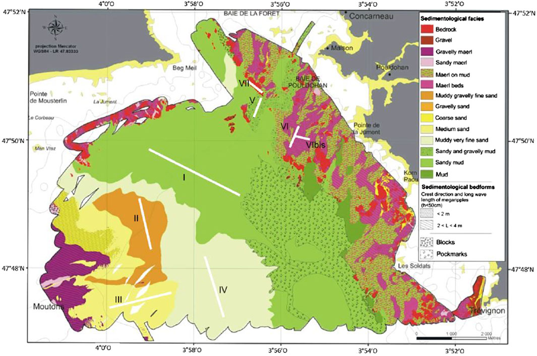
Figure 1. Sedimentology map of the Bay of Concarneau (Ehrhold et al., 2006). Straight white lines represent the geographic positions of the seven study areas.

Figure 2

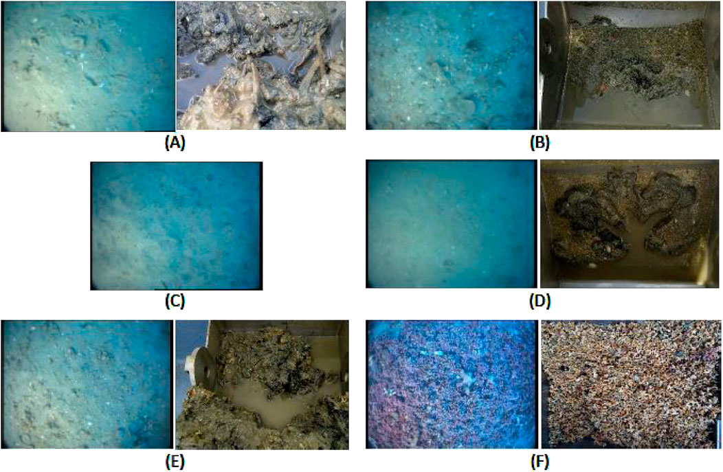
Figure 2. Seafloor sediment photos, including Site I [sandy mud (A)], Site II [muddy gravelly fine sand (B)], Site III [medium sand (C)], Site IV [muddy very fine sand (D)], Site V [sandy and gravelly mud (E)], and Site VI [maerl beds (F)]. For each site, a pair of images is shown, one from video footage and one from grab samples, except for Site III, which only has video. No video was taken at Site VII, which consists of rough rock.

2.2 Acoustic data collection and configurations

The surveys were conducted in March 2021 aboard the French coastal research vessel R/V Thalia. This vessel is specifically designed for coastal scientific missions and is equipped with advanced acoustic systems. It mainly features a Kongsberg EM 2040D Dual Receiver multibeam echosounder, providing high-resolution bathymetric and backscatter data. In addition to this MBES system, R/V Thalia can deploy a portable vertical pole on its starboard side, enabling the installation and operation of EK80 scientific echosounders mounted on a rotating device. This configuration facilitates the collection of complementary and simultaneously acoustic data collection for multispectral backscatter study and cross-calibration of the MBES.

2.2.1 EK80 collection and processing

For survey efficiency, up to three EK80 transducers were mounted simultaneously at the lower tip of the vertical pole installed on the ship’s side (Figure 3). This setup made possible a concurrent acquisition at three different frequencies. The transducerswere fixed to a remotely controlled pan-and-tilt mechanism, enabling precise adjustment of both horizontal and vertical angles with a practical accuracy of approximately 1°. For this experiment and as in (Fezzani et al., 2021), five Simrad EK80 wideband transceivers were used, each paired with a Simrad split-beam transducer operating at nominal frequencies of 38, 70, 120, 200, and 333 kHz. The transceivers were operated using two standard EK80 Wide Band Transceivers (WBT) (Demer et al., 2017), enabling simultaneous acoustic acquisition with two transceivers. To address installation constraints and minimize frequency interference, three different configurations were employed for transducers: an ES70-7C (45–90 kHz) paired with an ES200-7C (160–260 kHz), an ES120-7C (90–170 kHz) combined with an ES333-7C (280–450 kHz), and an ES38-10 (34–45 kHz) operated alone. These configurations collectively cover a frequency range fully spanning 34–450 kHz. For all transducers, the one-way beam aperture at nominal frequency is approximately 7°, except for the ES38-10, which has a beam aperture of 10°. In addition to using multiple transducers simultaneously, a specially-modified version of the acquisition software was employed, making possible the transmission of both continuous wave (CW) and frequency-modulated (FM) signals across a user-defined frequency range. In contrast, the standard EK80 software only supports CW signals at the nominal frequencies of the transducers. With this improvement we could operate up to eight frequencies for the first configuration, six frequencies for the second, and four frequencies for the ES38-10. Pulse lengths were typically set to 256 $\mu s$, ensuring an adequate signal-to-noise ratio (SNR), excepted for certain outer beam pointing angles of the 333-kHz transducer, where the pulse length was adjusted to 512 $\mu s$ to improve the SNR. Before the at-sea survey, the five EK80 were calibrated following the procedure outlined in (Demer et al., 2015) using a 25-mm diameter tungsten-carbide sphere. The calibration was carried out at the tank facility of the Institut Français de Recherche pour l’Exploitation de la Mer (IFREMER) in Brest. Akin to the setup aboard R/V Thalia, the EK80 transducers were mounted and steered using the same pan-and-tilt device during this in-tank calibration, following a protocol guided by the calibration functionality provided in the EK80 software. For each site, the survey strategy involved running each survey line in both directions, with the transducers steered to different angles for each pass. The tilt angles from vertical ranged from −9° to 15° in 3° increments to better capture the specular lobe shape, and then in 5° increments up to 75°. To optimize the survey duration, approximately 100 pings were logged for each frequency and pointing angle. This meant that the pointing angle was adjusted along the survey line, assuming the area was sufficiently homogeneous. Ideally, data would be logged along the entire line for each tilt angle to minimize backscatter variation across the area. However, this approach was found to be too time-consuming. The frequencies and pulse durations transmitted at the seven sites are detailed in Table 1. The complex-valued data from each quadrant of the split-beam transducers were stored in raw format after undergoing initial filtering and decimation by the EK80 WBT. The main processing steps to estimate the mean backscattering strength (BS) for each pointing angle are detailed in (Eleftherakis et al., 2018) and can be summarized as follows:

$•$ Conversion to Volume Backscattering Strength (Sv): the raw signal voltage values are converted to Sv (in dB), i.e., the standard output for EK80 software (Demer et al., 2017).

$•$ Estimation of Insonified Target Area and Directivity Function: these are calculated assuming a flat seafloor, which is a valid assumption for most of the survey areas except for rocky outcrops.

$•$ Derivation of Bottom Backscatter: the bottom backscatter is calculated using Equation 1.

$•$ Bottom Detection: the seafloor echosounding point position is identified for each ping using amplitude-maximum and phase-zero-crossing classical methods.

$•$ Snippet Extraction: backscatter samples are extracted within $\pm$ 1° from the nominal incidence angle of each ping.

$•$ Mean Backscatter Calculation: all snippets values are averaged to one single backscatter value for each pointing angle. For the final ARC, amplitude detection is applied for the specular region ($<$20°), while zero-crossing phase detection is used for the remaining angles.

Figure 3

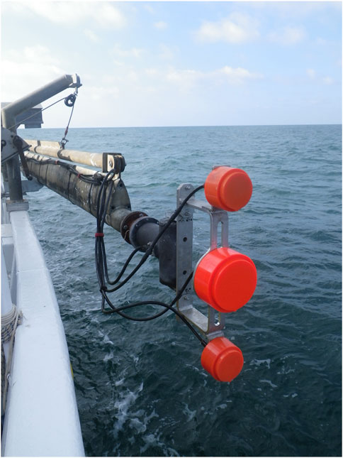
Figure 3. EK80 installation on the mobile vertical pole onboard RV Thalia. The pan-and-tilt system is fixed at the tip of the pole with the three EK80 transducers attached on a common supporting frame. The diameter of the center transducer (ES120-7C) is 18 cm.

Table 1

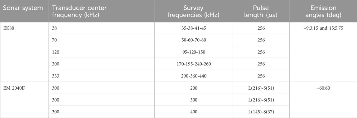
Table 1. Values of frequencies, pulse lengths and angles used during the surveys with EK80 and EM 2040D respectively.

As described in (Fezzani et al., 2021), a correction was applied to the SBES beam aperture to account for the ratio between the transducer’s nominal frequency and its actual operating frequency. The seafloor backscatter strength is calculated for each ping as follows:

$S_b=Sv+10{\log }_{10}\left(r^2\frac{c{T}_{\mathit{eff}}}{2}\psi {\left(\frac{{\nu }_n}{\nu }\right)}^2\right)-10{\log }_{10}A-D(1)$

where $Sv$ is the measured volume backscatter strength (in dB) calculated from the EK80 raw data files (Demer et al., 2017); $r$ is the sonar-target range (in meters); $\psi$ is the nominal equivalent aperture of the source/receiver system; $T_{\mathit{eff}}$ is the effective pulse length; ${\nu }_n$ and $\nu$ are the transducer nominal and actual operating frequencies, respectively; $A$ is the seabed insonified area; and $D$ the beam directivity function, which depends on the along-track and athwartship angles. This correction is not used for specular value, as the phase ramp is not stabilized.

In addition to the traditional method used to calculate the positions of the soundings and extract snippet samples, this paper introduces an alternative algorithm for bottom backscatter (BS) estimation. This new approach is based upon echo integration of the seafloor volume scattering strength $(Sv)$ samples (Equation 2). Unlike conventional techniques that directly extract and average snippet values, this method focuses on integrating the detected $Sv$ signal envelope across the whole seafloor echo. The proposed method offers potential improvements in backscatter accuracy by incorporating a more comprehensive set of $Sv$ data points, thereby reducing noise and enhancing the reliability of BS estimation. This effect is minimized at normal incidence, where the energetic maximum sample dominates the seafloor echo integration. However, for tilted acquisitions, the entire beam footprint is integrated, covering a much broader range of incidence angles on the seafloor, which smooths the ARC. A paper describing this approach at near nadir area has been submitted to the present special issue (Le Bouffant et al., 2025). Considering that, in the case of an echosounder tilted at an angle $\theta$, the beam footprint on the seafloor becomes $\frac{\psi }{\cos \theta }{R}^2$, Equation 6 from (Le Bouffant et al., 2025) lead to the general expression for $S_b$

$S_b=cos\theta {\displaystyle \sum _k}S{v}_k\frac{R_k^2}{R_{\mathit{det}}^2}dr(2)$

where $\theta$ is the tilt angle; $R$ the seafloor sample range and $R_{\mathit{det}}$ is the detection range of the seafloor (sounding point position). This method eliminates the need to account for various complex scenarios that can affect the standard computation of the insonified area at normal or near-normal incidence, where it is typically assumed that the entire beam footprint is fully covered by the pulse. However, in the case of short pulses, the pulse footprint may form an annulus before covering the entire beam footprint, or seafloor roughness may exceed the pulse length, preventing it from covering the seafloor in one pass (Le Bouffant et al., 2025). The echo-integration method no longer depends on specific pulse footprint timings and ensures that the entire beam footprint is covered and integrated over the effective pulse duration. The $Sv$ integration method offers a significant advantage by enabling the use of advanced signal processing techniques developed by the fisheries acoustics community for wideband signals in frequency modulation (FM) mode (Demer et al., 2017). Traditionally, bottom backscatter (BS) estimation has relied on narrowband acoustic systems, which provide limited spectral resolution. By adopting wideband processing, we open the possibility of conducting detailed multispectral analysis of the seafloor BS across a broader frequency range. This approach not only simplifies the workflow for multispectral BS studies but also drastically reduces the need for extensive data acquisition campaigns using tilted EK80 systems, which are typically required for multi-angle and multi-frequency backscatter measurements. The feasibility of this method will be further explored in a dedicated future publication.

In Figure 4, we present the comparison results of both methods presented above and applied at Site I. The results shown here are representative over all tested frequencies and sites. One can observe a maximum difference of about 1 dB in the near-nadir region, where the backscatter (BS) estimated using the amplitude detection method is slightly higher than the one derived from Sv integration. For the outer beams, the difference between the two methods decreases, remaining below 0.5 dB and tending toward zero at grazing angles. For the backscatter results presented in the following, we will rely on the values derived from the echo-integration method, as it proves to be more stable, particularly in situations where there is an insufficient number of pings per angle.

Figure 4

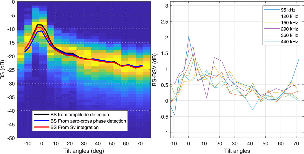
Figure 4. Comparison of the two methods of backscatter calculation applied to Site I data. The left figure shows the histograms of snippets amplitudes at 120 kHz as a function of angle, along with the angular responses estimated using either the amplitude detection method (black curve) or the zero-crossing phase detection (blue line), together with the result from Sv integration (red curve). The right figure illustrates the difference between the backscatter values estimated using the two methods—standard method and Sv echo-integration—across several frequencies; while the Sv method systematically underestimates the BS values, the bias reaches hardly 1 dB for most angles.

2.2.2 MBES collection and calibration

The data was collected using the Kongsberg EM 2040D multibeam echosounder installed on R/V Thalia. This MBES operates at three frequencies—200, 300, and 400 kHz—and features three transmit angular sectors with three primary modes of operation: ‘Central’ (only the central sector is active), ‘Normal’ (all three sectors are active), and ‘Scanning’. In this study, only the ‘Central’ mode was used, at all three frequencies and for both short and long pulse lengths. The continuous wave (CW) pulse length for the central sector ranges from 35 to 150 µs? During the survey, the system was fully roll- and pitch-stabilized, ensuring consistent beam performance. Due to time constraints, not all possible combinations of frequencies and pulse lengths could be applied across the entire surveyed area; the specific settings used in each case are detailed in Table 1. In order to compare the data from the MBES and the SBESs, a full calibration procedure of the MBES is necessary to provide accurate reference values for both the transmitted level and the receiving sensitivity. Since MBES measurements were conducted simultaneously with the fully-calibrated EK80, it was possible to cross-calibrate the MBES using data recorded by the SBES at the same frequencies and serving as reference curves (Eleftherakis et al., 2018). To achieve this cross-calibration, Site V was found to be the best choice among all the surveyed sites, since it offers a homogeneous and flat seafloor; these characteristics are ideal for ensuring that the comparison between the MBES and SBES data is not influenced by variations in the seafloor topography. Additionally, Site V is composed of coarse sediment, which tends to exhibit naturally a stable and nearly predictable Lambertian scattering response. The cross-calibration was performed using the SonarScope^® software developed by IFREMER (Augustin and Lurton, 2005). The compensation process was carried out in three stages (for further details, see (Eleftherakis et al., 2018)): 1) correcting transmission losses due to absorption, which vary with changing hydrological conditions; 2) adjusting for the instantaneous signal footprint area, considering factors such as incident angle, directivity pattern aperture, and pulse duration; and 3) estimating the array directivity patterns and applying specific gains to each angular sector of the echosounder based on the EK80 reference curve. This procedure was applied to the six configurations of the EM 2040D on Site V (three frequencies with two different pulse lengths). For the reference curves from the EK80, we used the closest EK80 frequency to the MBES frequency mode, resulting in 195 kHz measurements to calibrate the 200-kHz data of the MBES, 290 kHz for the 300-kHz data, and 440 kHz for the 400-kHz data. To build the reference curves from the EK80, we used the GSAB model (Lamarche et al., 2011) fitted to the tilt measurements in order to cover the full swath of the MBES. The cross-calibration results obtained at Site V for the 200-kHz frequency, using both short- and long-pulse settings, are presented in Figure 5. The presented results reveal biases ranging approximately from −1 to −5 dB. Notably, a difference of about 1 dB is observable between the two pulse types near nadir (within $\pm 15°$). These magnitudes are significant and emphasize the necessity of implementing an intensity-calibration procedure for this particular MBES model. Such a calibration process is crucial to correct the observed biases, ensuring that the backscatter measurements are accurate and consistent across different pulse settings.

Figure 5

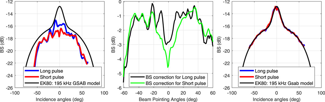
Figure 5. Cross-calibration results of the EM 2040 200-kHz mode on Site V. Left: Mean raw angular curves of the EM2040 with two pulses (Long and Short) and the reference GSAB model from the EK80 at 190 kHz. Middle: Estimated backscatter correction of each pulse. Right: final result illustrating the application of the calibration curves.

3 Results and discussion

3.1 Pulse length effect on the angular response curves

To study the effect of pulse length on the ARCs recorded by the EK80, a session of angular measurements was conducted between two at-sea surveys while the ship was anchored in the Bay of Concarneau. These measurements were performed using the two transducers, 70 and 200 kHz, with the same configurations as used on the survey sites. However, for these measurements, the pulse lengths were varied for each frequency between 256 $\mu s$, 512 $\mu s$, and 1,024 $\mu s$. For the EM 2040D, we attempted to vary the pulse length for each frequency from ‘Short’ to ‘Long’ on each site, whenever time permitted. Figure 6 presents the results for three frequencies on the anchoring area obtained with the EK80, as well as the results from the EM2040 at site V. For the EK80 data, no pulse effect is observed on the mean ARCs across all tested frequencies. In contrast, for the MBES, a variation in the ARCs can be observed between the two pulse lengths, also depending on frequency. This difference varies from 2 dB at a 200 kHz up to 4 dB at 400 kHz in the near-nadir area. This suggests a combined effect of wavelength and pulse. By analyzing these effects on the other sites, when available, we observe similar results with a dependency on the seafloor roughness of the region. This is particularly noticeable on the rocky and maerl areas, where the specular signals decrease at low incidence angles, especially for shorter pulse lengths and higher frequencies. The difference in ARCs at vertical incidence, as a function of pulse length, along with the dependence on roughness, suggests that it could be related to the computation of the insonified area in this cases. Classically, for MBES arrays, the along-track extent is defined by the Tx beamwidth, while the across-track extent is influenced by pulse length at oblique incidence and by the receiver beamwidth at normal incidence. Approximate formulas are commonly used for these calculations (Lurton, 2010) as:

$A_O=\phi R\frac{cT}{2\sin \theta \cos \gamma }(3)$

$A_N=\phi \omega R^2\frac{1}{\cos \theta \cos \gamma }(4)$

$A=\min \left(A_N,A_O\right)(5)$

Figure 6

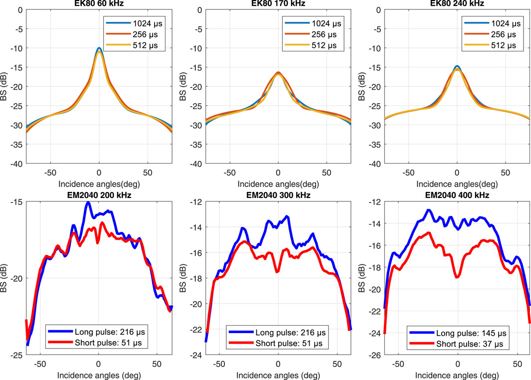
Figure 6. Backscatter curves vs incidence angle. Upper figures: EK80 results for 60, 170, and 240 kHz frequencies (from left to right). Three different pulse lengths were used for each case. Lower figures: Backscatter curves from the EM2040 system for 200, 300, and 400 kHz frequencies (from left to right). Two pulse lengths were used: short and long.

with $A_O$, $A_N$ and $A$ representing the insonified area at oblique incidence, near-normal incidence, and the overall area, respectively; R the range; $\phi$ and $\omega$ the along-track and across-track two-way equivalent apertures respectively; T the effective pulse length; c the sound speed; $\theta$ the incidence angle; and $\gamma$ the along-track seafloor slope. At oblique incidence (short-pulse regime) the insonified area calculation takes the pulse length into account (Equation 3), but this is not the case at normal incidence (long-pulse regime), where it is assumed that the acoustic footprint (then delimited by the beam aperture) is fully covered by the maximum pulse amplitude (Equation 4). In our case, the most constraining pulse is the ‘Short’ pulse at 400 kHz for the MBES, with a total length of 37 $\mu s$, equivalent to 14 $\mu s$ in effective pulse length. The effective pulse is available in the MBES raw data and calculated as for the EK80 (Andersen et al., 2024). For the results at Site V given in Figure 6, the depth of the area was approximately 19 m, with the MBES beam aperture around 1° by 1°. With the dimensions, the long-pulse regime near nadir remains valid even for the short pulse. However, with a range resolution around 1 cm (for 14 $\mu s$), micro-roughness variations exceeding the pulse length can prevent the entire seafloor footprint from being insonified at once. This leads to a discrepancy between the theoretical estimation of the insonified area (Equation 5) and the actual one. In such cases, the difference becomes more significant for shorter pulses. As the same formulas for insonified areas are used in the case of tilted EK80 measurements, this hypothesis could also explain the differences between the two algorithms presented above for estimating the ARC at near nadir area for EK80 measurements. Indeed, the echo-integration of the bottom backscatter method ensures full coverage of the projected beam pattern, thereby minimizing the effect of pulse length on the vertical backscatter estimation. Another factor that can explain the drop in specular reflections for short pulses is the possible inaccuracy in the bottom detection algorithm and hence the selection of snippet sections around the sounding detection instant. Indeed, for short pulses, the bottom signal at low incidence angles is very narrow and highly variable, which causes significant variations between snippets for one same beam. By analyzing the MBES snippets recorded around normal incidence, this phenomenon is easily noticeable in several successive pings. Near nadir, as few as only two to three samples per beam can correspond to the seafloor echo, while one can observe samples recorded in the water column; this obviously tends to lower the averaged backscatter per beam. All these observed variations with respect to frequency and pulse length highlight the paramount importance of calibrating multibeam echosounders before analyzing seabed backscatter data. Calibration ensures that the system’s responses are accurately accounted for, and reduces uncertainties caused by equipment-specific or environmental factors. This process is essential for obtaining reliable and comparable backscatter data, enabling precise characterization of seabed properties and supporting a wide range of applications, from sediment classification to habitat mapping.

3.2 MBES cross-calibration checking

To validate the calibration results, a straightforward approach involves comparing the compensation curves obtained across all survey sites, as they should, in theory, be identical. The EM2040 compensation curve derived at Site V was applied to correct the MBES data from the other sites using the Sonarscope^® software. The corrected data were then compared with the calibrated EK80 measurements taken at the closest matching frequencies at these same sites, over a limited range of tilt angles. Consistent agreement between these two independent datasets would confirm the accuracy of the EM2040 calibration procedure. Figure 7 presents the results of the comparison between the EK80 at 195 kHz and the EM2040 at 200 kHz across all areas, except for Area V, which was used for calibration. The detailed results for the other frequencies will be provided as supplementary data to this paper. For Site I, there is a good agreement between the average MBES curves for different pulse lengths and the corresponding SBES angular measurements. This consistency is observed across all tested frequencies. On Site II, the two calibrated systems also show good overall consistency. However, at 200 kHz, a difference of approximately 1 dB is observed within the angular range of 10°–50° (Figure 7). This discrepancy remains unexplained. For Sites III and IV, it was discovered during post-processing that the seabed reflectivity significantly varied along the two survey lines, leading to inconsistent measurement results for higher frequencies. The navigation path for each site was selected based on the sediment map shown in Figure 1, but it appeared that the boundaries between the different sediment types are not entirely accurate. This was verified for both zones by comparing the EK80 measurements with the average MBES curves after applying a mask to differentiate between the two sediment types along the survey line. As the EK80 tilt angle was adjusted multiple times on the same line, it was observed that the corresponding angular measurements alternately matched with types 1 and 2. For Sites VI and VII, corresponding to maerl and rocky substrates, respectively, we observe a good agreement between the two systems at 200 kHz, despite not accounting for incidence angles in the EK80 data. However, this agreement is less consistent at other frequencies, particularly in the case of the rocky substrate at 400 kHz, where the discrepancies become more pronounced. In this particular case, the discrepancy is not only observed between the two systems but also between the short pulse and the long pulse, despite proper calibration. The difference between the EK80 and the EM2040 can likely be attributed to the roughness of the rocky substrate and the absence of true incidence angle corrections for the EK80. On the other hand, the difference between the two pulse lengths, which is noticeable at 400 kHz but not at 200 kHz (no measurements were taken with the long pulse at 300 kHz), is relatively significant. In conclusion, the cross-calibration of the MBES can be considered as satisfactory, despite the fact that the measurements performed with the EK80 for comparison with other sites were not well-suited for this exercise. Indeed, due to survey time constraints, we assumed flat and homogeneous seabeds across all sites. Consequently, we altered the tilt angles of the EK80 along the same survey line and in both directions, which led to discrepancies between the two systems. An ideal comparison would involve performing angular measurements with the single-beam system in all directions (port and starboard) and along the entire survey line. However, this approach is highly time-consuming.

Figure 7

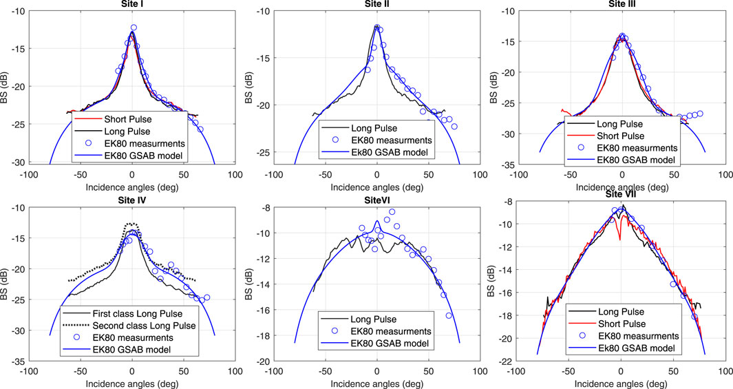
Figure 7. Cross-calibration validation on all sites for the EM2040 at 200 kHz. (blue dots) EK80 values at 195 kHz; (solid blue) GSAB model fit to the EK80 measurements; (solid black and red) mean ARC from EM 2040 after correction using the compensation curve determined at Site V.

3.3 Multispectral analysis

Figure 8 presents the GSAB model of EK80 angular measurements recorded at all frequencies over the seven study sites. At first glance, spectral variations are not uniform across sites. The maerl seabed (Site VI) exhibits the highest variation in backscatter (BS) levels across all angles. The difference in BS levels across frequencies ranges from 7 dB at nadir to more than 10 dB for the outer beams. Both the maerl and rocky sites exhibit weak specular components, with curves typical of hard rough interfaces. The ARCs for these two seabed types also display a frequency dependence varying little with angle, unlike other sites where lower frequencies result in a more pronounced specular response (Jackson and Richardson, 2007). The frequency dependence of the shape of the specular peak, of the plateau level, and of the fall-off at grazing angles also varies from one site to another, highlighting the contribution and relevance of multi-spectral backscatter analysis for seafloor characterization. To compare the reflectivity levels and the ARC shapes as a function of frequency among the different sediment types, Figure 9 presents the measured BS values at 45° and 0° of the GSAB model as well as the difference between the levels at 0° and 45° $(B{S}_{0°}-B{S}_{45°})$ for all frequencies. This figure also includes the results for maerl ripples, with surveys conducted in two directions parallel and perpendicular to the ridges (see Figure 1; note that the VIbis line direction was not surveyed with the 38 kHz transducer. The medium-sand data (Site III) exhibits the lowest BS level at 45° and remains constant around −25 dB for frequencies above 70 kHz. The variation in measurements between 170 and 260 kHz around the regression line is due to the variation in BS along the survey line at incidence angles around 45°. The sediments at Sites I and IV (sandy mud and muddy very fine sand, respectively) exhibit very similar BS levels at 45° for high frequencies ($<$ 100 kHz) and remain constant around −22 dB. The BS level for the Sites II and V sediments (muddy gravely fine sand and sandy gravely mud, respectively) continuously vary across the entire frequency range of the study. However, the BS level of the rock (Site VII) stabilizes beyond 80 kHz, around −13 dB. Site VI (maerl), surveyed in two perpendicular directions (parallel and perpendicular to the ridges direction), shows very similar BS values at 45°, demonstrating the consistency of the measurements. It should be noted that the azimuth effect on angular measurements generally occurs below 40° incidence. The BS level variation for maerl is the most significant, as shown in Figure 8; beyond 100 kHz, its level exceeds that of rock, reaching approximately −11 dB at the upper end of the frequency range. The analysis of the BS difference between the specular zone (at 0°) and the flat region of the angular response (at 45°) (Figure 9) shows, as expected, a more significant variation at lower frequencies. This variation is more pronounced for the softer sediments (Sites I to V). For the more consolidated minerals (rock and maerl), the variation is less pronounced and stabilizes beyond 60 kHz, which is consistent with Lambertian-shaped angular curves (see Figure 8). Site V (sandy and gravely mud), which can be considered a transition between soft and hard sediments, is distinguished by the disappearance of the specular shape beyond 170 kHz.

Figure 8

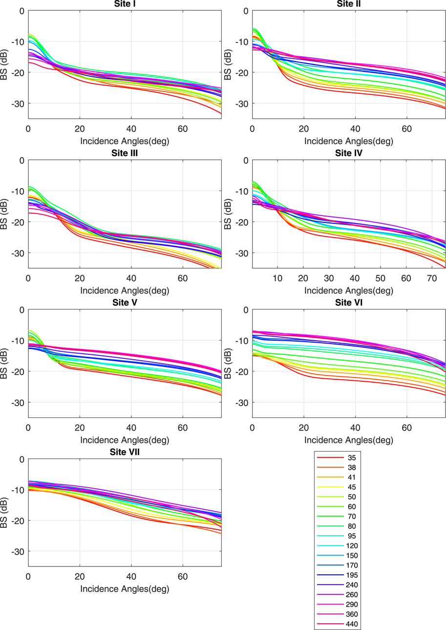
Figure 8. GSAB model fitted to measured BS values for all frequencies on the seven experimental sites. The average root mean square (rms) difference between the averaged experimental values and the fitted model shows a typical magnitude of 0.five to one dB.

Figure 9

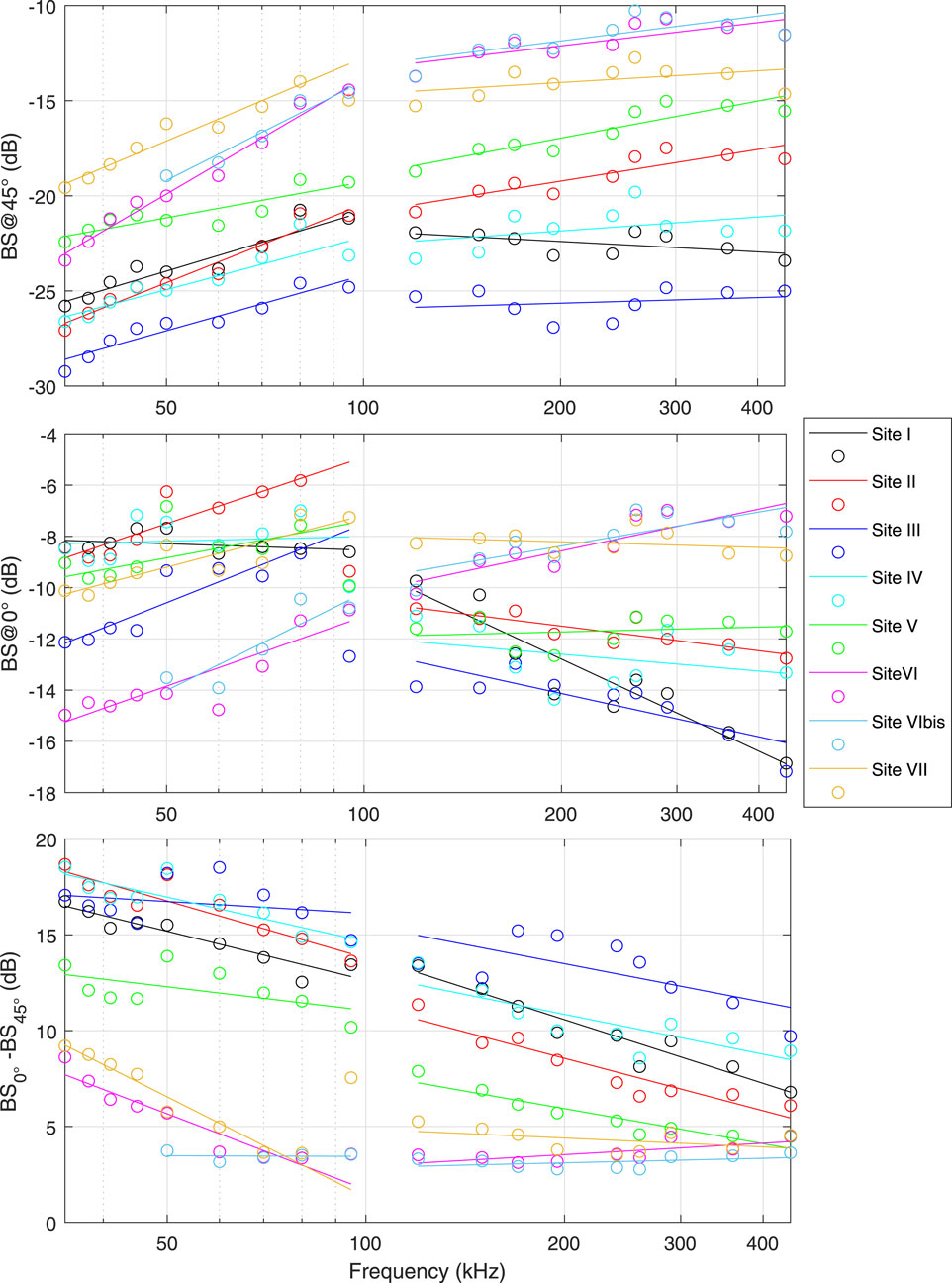
Figure 9. Bottom backscatter strength (BS) as a function of frequency for the seven study sites (color-coded). Top: BS at an incidence angle of 45°; Center: BS at normal incidence (0°); Bottom: Difference between BS at 0° and BS at 45°. Linear regression fits are overlaid on each plot.

Similarly to Fezzani et al. (2021); Wendelboe (2018); Weber and Ward (2015), the frequency dependence of backscatter strength can be analyzed through its spectral slope. Notable variations in this dependence were observed even within the same sediment type, indicating that the relationship between frequency and backscatter strength is not uniform across the full frequency range. To account for this variability, we estimated the spectral slope separately for frequencies below and above 100 kHz (based on linear fits), rather than assuming a single slope over the entire bandwidth. The resulting slope values for each frequency range are reported in Table 2, along with a comparison to the slope computed over the full frequency band. A spectral slope of 1 corresponds to a variation of 3 dB per octave. This approach enables a more accurate characterization of frequency-dependent scattering behavior, which may provide insight into the physical properties of the seafloor.

Table 2

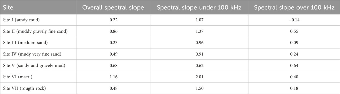
Table 2. Spectral slope values at 45° incidence angle on the seven sites.

As expected, the spectral slope for frequencies below 100 kHz is higher than that above 100 kHz. This trend holds for all sites except for Site V (see Table 2). The backscatter strength varies between $BS\propto 10{\log }_{10}{f}^{0.62}$ and $BS\propto 10{\log }_{10}{f}^{2.01}$ for low frequencies, corresponding to sandy gravelly mud and maerl, respectively. At high frequencies, BS ranges from $BS\propto 10{\log }_{10}{f}^{-0.14}$ to $BS\propto 10{\log }_{10}{f}^{0.64}$, corresponding to sandy mud and sandy gravelly mud, respectively.

For all sites—including rocky seabeds—the frequency dependence above 100 kHz is below 1 dB/octave, with the exception of Site II (muddy gravelly fine sand), Site V (sandy gravelly mud), and Site VI (maerl habitat), where it can reach up to 2 dB/octave. This stronger frequency dependence may be attributed to surface roughness effects that become more pronounced at higher frequencies, especially in the presence of gravel and maerl.

At nadir (Figure 9), the frequency dependence is similar to that observed at 45°, again exhibiting a change in trend between frequencies below and above 100 kHz. However, a clear discontinuity is observed between 80 kHz and 120 kHz, with a transition around 95 kHz that can reach up to 5 dB. Generally, a positive slope is observed at low frequencies across all sites, followed by a flat or negative slope at higher frequencies, except at Sites I and VI. The maerl habitat (Site VI) consistently shows a positive slope across the entire frequency range. In contrast, Site I (sandy mud) exhibits a near-zero slope below 100 kHz, but at higher frequencies shows a strong negative frequency dependence, with a slope of approximately −4 dB/octave. Notably, Site I is also the only sediment type to exhibit a negative slope at 45° for high frequencies (see Table 2).

3.4 Comparison with results from other studies

Several recent studies have reported absolute backscatter values recorded at a 45° incidence angle for various seafloor habitats. In our previous work Fezzani et al. (2021), we conducted similar measurements at discrete frequencies ranging from 45 to 450 kHz across four homogeneous areas with different sediment types. Weber and Ward (2015) performed measurements using a calibrated 200-kHz EK80 SBES operating in frequency modulation (FM) mode (170–250 kHz) in an area characterized by fine sand, gravel, and pebbles. Wendelboe (2018) analyzed average seabed backscatter strength over a frequency range of 190–400 kHz on a medium sand area, using an in-tank calibrated multibeam echosounder. Trzcinska et al. (2021) operated a calibrated MBES at 150 kHz to measure averaged backscatter across different sediment types, including fine sand, gravelly sand, and boulders. In a recent study (Roche et al., 2025), we conducted additional measurements using a tilted EK80 on the Kwinte reference area (Belgian coast) with frequency ranges from 50 to 440 kHz. This area is characterized by sandy gravel with shells. To facilitate a comparison between our backscatter measurement results and other recent studies, we have compiled and summarized the reported backscatter values at a 45° incidence angle from these works in Figure 10 providing an overview of the measured values across different sediment types and frequency ranges. The angular dependence of sediments studied in our previous paper (Fezzani et al., 2021) shows a strong similarity between gravelly sand with coarse elements and the values observed for rough rock at Site VII across the entire frequency range. Gravelly mud with shells and silty sand with shells both exhibit characteristics very similar to those observed on the Kwinte area for sandy gravel with shells. The frequency-dependent curve for these three areas lies between the curve of Site V (sandy and gravelly mud) and the rough rock of Site VII. Finally, the values for the mud to sandy mud area are highly comparable to those observed at Site IV, which is characterized by muddy very fine sand sediments.

Figure 10

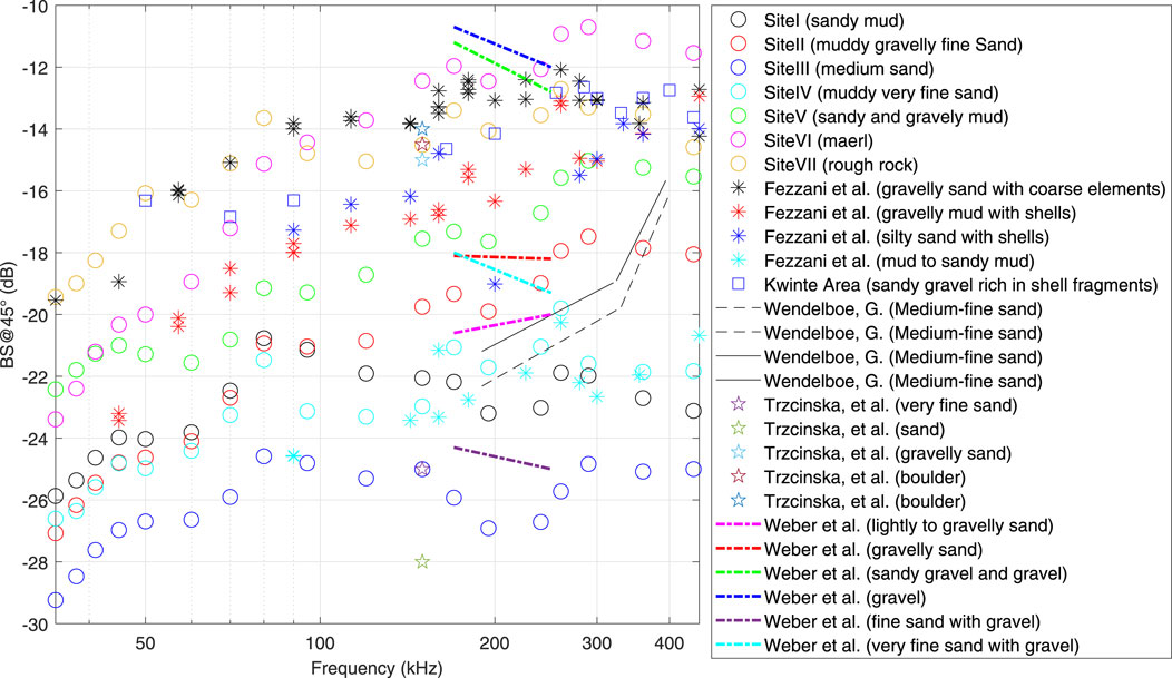
Figure 10. Summary of seafloor backscatter strength at 45° incidence versus frequency, obtained by various authors with calibrated acoustic systems.

The results obtained by Weber and Ward (2015) over the frequency range 170–250 kHz, using a calibrated EK80 at 45°, illustrate the difficulty of obtaining a reliable estimate of the spectral slope over a half-octave bandwidth. Indeed, across the six studied areas, BS values vary by approximately 1 dB between the beginning and end of the frequency range, making extrapolation to a broader bandwidth challenging, despite the use of FM mode. This issue is particularly evident in the intra-transducer level variations observed in our case, where the relative slopes may significantly deviate from the overall trend. Therefore, we estimate that a bandwidth of at least one octave is necessary to properly assess frequency dependence, especially at high frequencies ($>$100 kHz). However, the measured levels around 200 kHz for the two hard sediment zones (sandy pebble gravels) are very close to those observed for maerl in our study. The areas characterized by fine to medium sand with shells and pebbly very fine sand exhibit levels similar to those observed at Site II (muddy gravelly fine sand) and Site V (sandy and gravelly mud). Finally, the fine sand zone is comparable to the medium sand site in our study with about −15 dB at 200 kHz. The study presented by Trzcinska et al. (2021), using a calibrated Norbit multibeam system at 150 kHz, shows that BS values at 45° for boulder and gravelly sand sediments are very similar to those obtained for rock in our study. Similarly, the −25 dB value reported for very fine sand matches perfectly with our results for medium sand (site III). However, the −28 dB value reported for sand is lower than all other values compared in Figure 10. The authors attributed these lower values to a possible micro-roughness effect caused by small-scale sand ripples. The results obtained in Wendelboe (2018) were collected using a SeaBat T50 multibeam system, calibrated in both transmission and reception in a controlled tank environment. The data were acquired over a fine to medium sand seabed, covering a frequency range from 190 kHz up to 400 kHz by 10-kHz steps. The obtained values are close to those of Site IV (muddy very fine sand) and are 3–4 dB higher than the values for medium sand (Site III) in the 200–300 kHz range. The author reported a similar magnitude of difference compared to a previous study conducted in the same area. Additionally, the author noted a change in spectral slope around 330 kHz, as shown in Figure 10. However, this behavior was not observed in any of the seven areas studied in our case. Instead, the values observed across all sites beyond 300 kHz exhibit either a flat or slightly negative slope.

The comparison of our backscatter measurements with recent studies highlights a strong consistency in the frequency-dependent behavior of different sediment types, particularly at a 45° incidence angle. Our results align well with previous findings, especially for hard substrates. A notable observation is that certain coarse sediments, such as maerl, pebbles, and boulders, can exhibit backscatter levels exceeding those of rock at high frequencies ($>$200 kHz), reaching values between −13 dB and −11 dB. This suggests that, at these frequencies, factors such as grain structure, porosity, and micro-roughness play a significant role in scattering properties. Additionally, this comparison confirm that the presence of shell fragments within sediment mixtures, even in fine-grained environments, leads to an increase in backscatter values. This effect is particularly evident in fine to medium sand with shells (Weber and Ward, 2015), where BS values are comparable to those observed at Sites II and V, which contain gravelly elements. Furthermore, our analysis reveals that pure sediments generally exhibit lower backscatter levels compared to mixed sediments, even when composed of fine particles. This trend is observed for medium sand (Site III), fine sand (Weber and Ward, 2015), and very fine sand (Trzcinska et al., 2021), all of which show lower BS values than mixed sediments with comparable grain sizes.

4 Conclusion

This study presents a comprehensive multispectral analysis of seafloor backscatter using calibrated single-beam and multibeam echosounders across a wide frequency range (35–440 kHz). By integrating multiple acoustic systems, we confirmed the feasibility of cross-calibrating MBES backscatter using SBES as a reference, ensuring reliable and consistent measurements across different frequencies and sediment types. Our results also highlight the impact of frequency and pulse length on Angular Response Curves, emphasizing the necessity of the calibration procedure for backscatter analysis. Our analysis, conducted over a wide frequency range covering most of the frequencies used by seafloor-mapping echosounders, and across various seabed types, highlights the challenges associated with frequency dependence analysis, both at nadir and within the stable part of ARCs around 45°. The variation in frequency-dependence rates between frequencies below and above 100 kHz, as evidenced in this study, further complicates the interpretation of acoustic wave interactions with different seafloor sediment types as a function of frequency. The comparison with results from several previous studies confirms the robustness of our past and present datasets and methodology, with observed backscatter levels aligning well with independent measurements from different calibrated acoustic systems. These calibrated measurements could be shared with the scientific community as a starting point of an e-Catalogue project under the BSWG working group. A template for data description is provided in the Supplementary Data of this paper, facilitating the integration of our dataset into a standardized framework for future studies. These findings hopefully contribute to advancing seabed classification methodologies by refining acoustic parameter databases and improving the reliability of frequency-dependent backscatter models. Overall, our study contributes to the growing body of work on multispectral backscatter analysis, providing valuable insights into the acoustic response of diverse seafloor habitats.

Data availability statement

The original contributions presented in the study are included in the article/Supplementary Material, further inquiries can be directed to the corresponding author.

Author contributions

RF: Formal Analysis, Methodology, Software, Writing – original draft, Writing – review and editing. LB: Formal Analysis, Methodology, Software, Writing – review and editing. NL: Formal Analysis, Methodology, Software, Writing – review and editing. XL: Formal Analysis, Methodology, Software, Writing – review and editing.

Funding

The author(s) declare that financial support was received for the research and/or publication of this article. This work was conducted in the framework of IFREMER Research and development Project $R403-006$ (Underwater Acoustics).

Acknowledgments

The authors would like to express their gratitude to Axel Ehrhold (Ifremer) for providing the necessary reports for the sedimentological interpretation of the study areas. We also thank Kongsberg Maritime for making available a special version of their software, allowing the use of the EK80 at different frequencies in CW mode. Finally, we extend our sincere appreciation to the R/V Thalia crew for their dedication and support during the sea measurement campaigns.

Conflict of interest

The authors declare that the research was conducted in the absence of any commercial or financial relationships that could be construed as a potential conflict of interest.

Generative AI statement

The author(s) declare that no Generative AI was used in the creation of this manuscript.

Publisher’s note

All claims expressed in this article are solely those of the authors and do not necessarily represent those of their affiliated organizations, or those of the publisher, the editors and the reviewers. Any product that may be evaluated in this article, or claim that may be made by its manufacturer, is not guaranteed or endorsed by the publisher.

Supplementary material

The Supplementary Material for this article can be found online at: https://www.frontiersin.org/articles/10.3389/frsen.2025.1574996/full#supplementary-material

References

Andersen, L. N., Chu, D., Handegard, N. O., Heimvoll, H., Korneliussen, R., Macaulay, G. J., et al. (2024). Quantitative processing of broadband data as implemented in a scientific split-beam echosounder. Methods Ecol. Evol. 15, 317–328. doi:10.1111/2041-210x.14261

CrossRef Full Text | Google Scholar

Augustin, J.-M., and Lurton, X. (2005). Image amplitude calibration and processing for seafloor mapping sonars. Eur. Oceans 2005 (IEEE) 1, 698–701 Vol. 1. doi:10.1109/oceanse.2005.1511799

CrossRef Full Text | Google Scholar

Brown, C. J., Beaudoin, J., Brissette, M., and Gazzola, V. (2019). Multispectral multibeam echo sounder backscatter as a tool for improved seafloor characterization. Geosciences 9, 126. doi:10.3390/geosciences9030126

CrossRef Full Text | Google Scholar

Clarke, J. H., Danforth, B., and Valentine, P. (1997). “Areal seabed classification using backscatter angular response at 95 khz,” in SACLANTCEN conf on high frequency acoustics in shallow water, 243–250.

Google Scholar

Demer, D., Andersen, L., Bassett, C., Berger, L., Chu, D., Condiotty, J., et al. (2017). Evaluation of a wideband echosounder for fisheries and marine ecosystem science. ICES Coop. Res. Rep. doi:10.17895/ices.pub.2318

CrossRef Full Text | Google Scholar

Demer, D. A., Berger, L., Bernasconi, M., Bethke, E., Boswell, K., Chu, D., et al. (2015). Calibration of acoustic instruments.

Google Scholar

Ehrhold, A., Hamon, D., and Guillaumont, B. (2006). The REBENT monitoring network, a spatially integrated, acoustic approach to surveying nearshore macrobenthic habitats: application to the Bay of Concarneau (south brittany, France). ICES J. Mar. Sci. 63, 1604–1615. doi:10.1016/j.icesjms.2006.06.010

CrossRef Full Text | Google Scholar

Eleftherakis, D., Berger, L., Le Bouffant, N., Pacault, A., Augustin, J.-M., and Lurton, X. (2018). Backscatter calibration of high-frequency multibeam echosounder using a reference single-beam system, on natural seafloor. Mar. Geophys. Res. 39, 55–73. doi:10.1007/s11001-018-9348-5

CrossRef Full Text | Google Scholar

Feldens, P., Schulze, I., Papenmeier, S., Schönke, M., and Schneider von Deimling, J. (2018). Improved interpretation of marine sedimentary environments using multi-frequency multibeam backscatter data. Geosciences 8, 214. doi:10.3390/geosciences8060214

CrossRef Full Text | Google Scholar

Fezzani, R., and Berger, L. (2018). Analysis of calibrated seafloor backscatter for habitat classification methodology and case study of 158 spots in the bay of biscay and celtic sea. Mar. Geophys. Res. 39, 169–181. doi:10.1007/s11001-018-9342-y

CrossRef Full Text | Google Scholar

Fezzani, R., Berger, L., Le Bouffant, N., Fonseca, L., and Lurton, X. (2021). Multispectral and multiangle measurements of acoustic seabed backscatter acquired with a tilted calibrated echosounder. J. Acoust. Soc. Am. 149, 4503–4515. doi:10.1121/10.0005428

PubMed Abstract | CrossRef Full Text | Google Scholar

Fonseca, L., and Mayer, L. (2007). Remote estimation of surficial seafloor properties through the application angular range analysis to multibeam sonar data. Mar. Geophys. Res. 28, 119–126. doi:10.1007/s11001-007-9019-4

CrossRef Full Text | Google Scholar

Gaida, T., Tengku Ali, T., Snellen, M., Amiri-Simkooei, A., van Dijk, T., and Simons, D. (2018). A multispectral bayesian classification method for increased acoustic discrimination of seabed sediments using multi-frequency multibeam backscatter data. Geosciences 8, 455. doi:10.3390/geosciences8120455

CrossRef Full Text | Google Scholar

Heaton, J. L., Rice, G., and Weber, T. C. (2017). An extended surface target for high-frequency multibeam echo sounder calibration. J. Acoust. Soc. Am. 141, EL388–EL394. doi:10.1121/1.4980006

PubMed Abstract | CrossRef Full Text | Google Scholar

Hughes Clarke, J. (2015). “Multispectral acoustic backscatter from multibeam, improved classification potential,” in Proceedings of the United States hydrographic conference (San Diego, CA, USA), 15–19.

Google Scholar

Jackson, D., and Richardson, M. (2007). High-frequency seafloor acoustics. Springer Science and Business Media.

Google Scholar

Janowski, L., Trzcinska, K., Tegowski, J., Kruss, A., Rucinska-Zjadacz, M., and Pocwiardowski, P. (2018). Nearshore benthic habitat mapping based on multi-frequency, multibeam echosounder data using a combined object-based approach: a case study from the rowy site in the southern baltic sea. Remote Sens. 10, 1983. doi:10.3390/rs10121983

CrossRef Full Text | Google Scholar

Lamarche, G., Lurton, X., Verdier, A.-L., and Augustin, J.-M. (2011). Quantitative characterisation of seafloor substrate and bedforms using advanced processing of multibeam backscatter—application to cook strait, New Zealand. Cont. Shelf Res. 31, S93–S109. doi:10.1016/j.csr.2010.06.001

CrossRef Full Text | Google Scholar

Lanzoni, J. C., and Weber, T. C. (2012). Calibration of multibeam echo sounders: a comparison between two methodologies. In European Conference on Underwater Acoustics. 835 (AIP Publishing), 17.

Google Scholar

Le Bouffant, N., Berger, L., and Fezzani, R. (2025). Using seafloor echo-integrated backscatter for monitoring single beam echosounder calibration. Front. Remote Sens. 6, 1549238. doi:10.3389/frsen.2025.1549238

CrossRef Full Text | Google Scholar

Lecours, V., Misiuk, B., Butschek, F., Blondel, P., Montereale-Gavazzi, G., Lucieer, V. L., et al. (2025). Identifying community-driven priority questions in acoustic backscatter research. Front. Remote Sens. 5, 1484283. doi:10.3389/frsen.2024.1484283

CrossRef Full Text | Google Scholar

Lurton, X. (2010). An introduction to underwater acoustics: principles and applications. 2nd edn. Springer.

Google Scholar

Lurton, X., Eleftherakis, D., and Augustin, J.-M. (2018). Analysis of seafloor backscatter strength dependence on the survey azimuth using multibeam echosounder data. Mar. Geophys. Res. 39, 183–203. doi:10.1007/s11001-017-9318-3

CrossRef Full Text | Google Scholar

Lurton, X., Lamarche, G., Brown, C., Lucieer, V., Rice, G., Schimel, A., et al. (2015). “Backscatter measurements by seafloor-mapping sonars,” in Guidelines and recommendations 200. doi:10.5281/zenodo.10089261

CrossRef Full Text | Google Scholar

Porskamp, P., Young, M., Rattray, A., Brown, C. J., Hasan, R. C., and Ierodiaconou, D. (2022). Integrating angular backscatter response analysis derivatives into a hierarchical classification for habitat mapping. Front. Remote Sens. 3, 903133. doi:10.3389/frsen.2022.903133

CrossRef Full Text | Google Scholar

Roche, M., Lønmo, T. I. B., Fezzani, R., Berger, L., Deleu, S., Bisquay, H., et al. (2025). Instrumental temperature-dependence of backscatter measurements by a multibeam echosounder: findings and implications. Front. Remote Sens. 6, 1572545. doi:10.3389/frsen.2025.1572545

CrossRef Full Text | Google Scholar

Trzcinska, K., Tegowski, J., Pocwiardowski, P., Janowski, L., Zdroik, J., Kruss, A., et al. (2021). Measurement of seafloor acoustic backscatter angular dependence at 150 khz using a multibeam echosounder. Remote Sens. 13, 4771. doi:10.3390/rs13234771

CrossRef Full Text | Google Scholar

Weber, T. C., and Ward, L. G. (2015). Observations of backscatter from sand and gravel seafloors between 170 and 250 khz. J. Acoust. Soc. Am. 138, 2169–2180. doi:10.1121/1.4930185

PubMed Abstract | CrossRef Full Text | Google Scholar

Wendelboe, G. (2018). Backscattering from a sandy seabed measured by a calibrated multibeam echosounder in the 190–400 khz frequency range. Mar. Geophys. Res. 39, 105–120. doi:10.1007/s11001-018-9350-y

CrossRef Full Text | Google Scholar