Integrating the landscape scale supports SAR-based detection and assessment of the phenological development at the field level

Climate change and increasing weather and seasonal dynamics challenge agricultural landscapes. To cope with this challenge information on crop performance is key. This study presents a novel framework for bridging landscape-scale vegetation dynamics with field-level crop phenology using Sentinel-1 radar time series. Unlike previous approaches that focus on local algorithm optimisation or SAR feature selection, this work integrates two scales: (1) landscape patterns derived from annual distributions of time series metrics (TSMs) and (2) field-level phenology, both linked to growing degree days (GDD). TSMs were generated through breakpoint analyses over different smoothing intensities for Sentinel-1 polarisation (PolSAR) and interferometric coherence (InSAR) features, capturing crop, orbit and sensor-specific responses. The framework quantifies uncertainties inherent in both remote sensing and ground observations, and evaluates trackable progress (phenological stage detectability) and tracking range (GDD variance around stages) to assess accuracy under variable acquisition geometries, weather and smoothing parameters. Applied to the DEMMIN site (Germany), the analysis revealed consistent TSM-GDD relationships for wheat, rape, and sugar beet, with descriptors such as soil fertility and water availability explaining spatial patterns (R² ≈ 0.8). Key novelties include the identification of low tracking ranges in drought years, the demonstration of the impact of orbit-specific incidence angles on monitoring fidelity, and the highlighting of Sentinel-1’s ability to resolve phenological variance across fragmented landscapes. By harmonising multi-scale SAR time series with agro-meteorological data, this approach advances transferable methods for operational crop monitoring, supporting precision agriculture and regional yield assessment beyond localised models.

1 Introduction

Crop phenology is an essential variable, when assessing plant health and productivity in the context of climate change and adaptation (Sakamoto et al., 2013; Whitcraft et al., 2019). Earth observation (EO), in particular optical data has demonstrated its potential to provide extensive information on the phenological progress of crop (Htitiou et al., 2024) s. In the last decade Synthetic Aperture Radar (SAR) emerged as an additional and reliable data source, due to its cloud penetrating capabilities (Canisius et al., 2018; Mascolo et al., 2024; Steele-Dunne et al., 2017). This development has been accelerated by the launch of ESA’s Sentinel-1 (S1). Its twin constellation generated SAR data of high temporal resolution, which can be used to assess crop development every 6 days over Europe (ESA, 2013). The potential of such data has been explored in several studies (e.g., Harfenmeister et al., 2021a; Khabbazan et al., 2019; Schlund and Erasmi, 2020).

However, in situ data of varying quality in terms of spatiotemporal coverage and accuracy challenge these studies. Some conducted their own field campaigns (Canisius et al., 2018; Harfenmeister et al., 2021b), which are time-consuming and labour-intensive. Other studies employed data obtained from national phenological monitoring frameworks (d’Andrimont et al., 2020; Lobert et al., 2023). Most of them are point data that depending on the sampling design do not necessarily reflect the heterogeneity within a field. For instance, phenological data provided by the German Weather Service (DWD) which has been frequently used in previous studies (Htitiou et al., 2024; Lobert et al., 2023; Schlund and Erasmi, 2020), do not follow a strict observation scheme, but employ volunteers that follow guidelines. In case of the DWD observation it is recommended to visit the fields two to three times per week and a phenological stage is only considered reportable if 50% of the field arrived at that stage. Moreover, the reported observations are not linked to a specific field, but refer to a two-to-five-kilometre radius around the assigned coordinates (Kaspar et al., 2015). These are all factors that are not clearly represented by calibration or validation approaches that are solely based on the difference between estimated phenology and observed phenology (Khabbazan et al., 2019; Löw et al., 2021; Schlund and Erasmi, 2020). It also has to be noted that the spatial density of DWD in situ observations conducted by volunteers has been decreasing over time.

In addition, SAR time series contain multiple uncertainties, which are introduced by environmental, system-inherent or user-defined factors. Varying environmental conditions are e.g., expressed by precipitation pattern or terrain parameters (Small, 2011). System-inherent aspects include acquisition geometry and speckle (Arias et al., 2022; Woodhouse, 2006), while user-defined settings refer to e.g., the length of observation period or smoothing intensity (Löw et al., 2024). All the above-mentioned factors warrant the consideration of alternative time series interpretations. Moreover, these issues exacerbate the comparability of field-based studies, the transferability and generalisation of the approaches and thus impede the knowledge transfer to praxis-oriented applications (Povey and Grainger, 2015).

Therefore, this study proposes a concept to generate information on phenological development at the field level with intentionally reduced dependency on in situ observations, while considering the previously mentioned uncertainties. Such a comprehensive approach to S1-based time series analysis is not represented in the current literature (Mandal et al., 2020; Mascolo et al., 2024; Schlund, 2025; Wang et al., 2024). For generating insights into crop development of varying degree of detail, the core of the concept is an overlay analysis of time windows at landscape and field level. Methodologically, the study extends Löw et al. (2024), which investigated the occurrences of time series metrics (TSM) of S1 time series in relation to acquisition geometry and crop specific phenological developments across multiple years. Thereby, relevant time windows of phenological change at landscape level were identified. Also, the resulting favourable S1 feature and orbit combinations for tracking crop phenology are utilized in the study at hand. The question of inherent uncertainties is addressed by establishing indicators that describe the agreement between TSM occurrences at field and landscape level as well as the trackable progress and tacking range covered by TSM for specific stages of DWD in situ observations. Furthermore, multiple orbits and S1 features (backscatter, coherence, decomposition) were integrated to produce insights into dominant tendencies within the overlay of landscape and field patterns, thus enabling the assessment whether a field is generally ahead or behind the landscape level development. Hereby, the concept adapts the baseline of growing degree days (GDD) in Löw et al. (2024) and further develops the ideas of describing phenological progress in relative terms, such as crop maturity (McNairn et al., 2018) and characterizing field specific developments in reference to a wider spatial context (Nasrallah et al., 2019). In a plausibility analysis that can also serve as a demonstrator of the concept’s applicability, the spatial distribution of the indicators is investigated in relation to environmental factors via correlation and variable importance analysis. These factors include terrain, weather and vegetation dynamics as well as soil properties. This concept can help improve on-farm management tools and landscape wide assessments of agricultural seasons by describing and monitoring phenological progress without the need for extensive in situ data collection.

2 Materials and methods

2.1 Study area and in situ data

The region of interest is situated in north-eastern Germany within the federal state of Mecklenburg West Pomerania (Figure 1). Characterized by an average annual precipitation of 550 mm and a mean air temperature of 8.3 °C, its climate is classified as temperate Middle-European. By 2001 the German Aerospace Center (DLR) established the Durable Environmental Multidisciplinary Monitoring Net Information Network (DEMMIN), which serves as a calibration and validation site for Earth observation missions (Spengler et al., 2018). DEMMIN is also part of the Joint Experiment for Crop Assessment and Monitoring (JECAM) network (Hosseini et al., 2021).

Figure 1

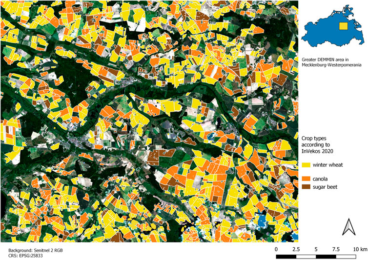
Figure 1. Map of InVekoS data 2020 for DEMMIN and selected crops: wheat, canola and sugar beet.

For the growing seasons from 2017 to 2021, information on parcel delineation and crop types in the DEMMIN area was extracted from the German integrated administration and control system (InVeKoS) of Mecklenburg West Pomerania. Winter wheat, canola and sugar beet are major crop types in DEMMIN. They belong to the seven area dominating crop types in Germany and were hence selected for this study. Only fields of significant size (>3 ha) were chosen to minimize pixel contamination from neighbouring land use or cover as previously described (Lobert et al., 2023; Löw et al., 2024).

Phenological in situ observations were obtained from the voluntary-based observer framework of the DWD (Kaspar et al., 2015). Any phenological developments recorded by DWD were translated to the BBCH (Biologische Bundesanstalt für Land-und Forstwirtschaft, Bundessortenamt und CHemische Industrie) scale, i.e., a classification scheme for measuring phenological development (Meier, 2001) to facilitate comparison with other studies. These observations encompass emergence, leaf development and canopy closure of sugar beet, stem elongation (BBCH 30), heading (BBCH 50), yellow ripening (BBCH 87) and harvest (BBCH 99) for winter wheat as well as inflorescence (BBCH 50), start (BBCH 60) and end of flowering (BBCH 69) and harvest (BBCH 99) of canola. This dataset was used to analyse approximately 500 field of winter wheat, 300 fields of canola and 150 fields of sugar beet per year. Due to the area’s poor coverage by this monitoring setup in terms of proximity and crop variety, the average occurrence date by federal state served as source of validation.

2.2 Growing degree data

Growing degrees are characterized as heat units and serve as a widely utilized tool for elucidating the progression of biological processes (McMaster and Wilhelm, 1997). Growing degree days (GDD) represent the cumulative sum of these units employed to model crop growth. They were also used in remote-sensing based studies to translate crop phenology into crop maturity for integration into crop yield models (McNairn et al., 2018). However, classical GDD approaches rely on a minimum base temperature only and neglect an upper temperature limit for plant growth. Especially conditions of extreme temperatures and variability can lead to errors when using those GDD approaches for phenological assessments (Ritchie and Nesmith, 2015; Stinner et al., 1974; Zhou and Wang, 2018).

Given our observation period, which includes years marked by extreme drought in Germany (Harfenmeister et al., 2021b; Schlund and Erasmi, 2020) the method proposed by Zhou and Wang (2018) was selected for meteorological assessments of GDD. This method addresses the shortcoming by the calculation of hourly temperature time (HTT) series with four key parameters: T_h (hourly measurement of air temperature), T_u (upper temperature limit), Topt (optimal temperature for maximum growth), and T_b (base temperature) (Zhou and Wang, 2018). By implementing an optimal threshold and an upper temperature limit to HTT calculation it can reflect heat and other temperature related stress, because less or no additional HTT are accumulated (see Equation 1).

$HTT=\left\{\begin{array}{c}0,T_h<T_b\\ {\left[\frac{T_h-T_b}{T_{opt}-T_b}\right]\left[\frac{T_u-T_h}{T_u-T_{opt}}\right]}^{\frac{T_u-T_{opt}}{T_{opt}-T_b}}\left|\right.T_b\le T_h\le T_u\\ 0,T_u<T_h\end{array}\right.(1)$

Data on air temperature is provided by DWD for the entire observation period (2017–2021) as an interpolated raster derived from the sensor network of DEMMIN (Haßelbusch and Lucas-Mofat, 2021). The native spatial resolution of the dataset is 250 m × 250 m per pixel, its temporal resolution is one hour and it was interpolated by employing ordinary kriging. Further details can be found in this DWD-report (Haßelbusch and Lucas-Mofat, 2021). Thus, the GDD are then calculated as cumulative sum of daily mean HTT based on this dataset. These calculations were conducted on an open data cube platform (ODC) (Killough, 2018) using the programming language Python. Table 1 specifies the thresholds of air temperature by crop type according to named references.

Table 1

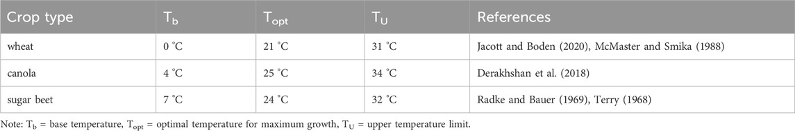
Table 1. Specifications of thresholds of air temperature for calculating GDD.

We used values derived from literature, because no data on strains and phenotypes for the investigated crop was available for that time period and area.

2.3 Sentinel-1 (S1) time series

The time series of S1 data encompasses relative orbits 146, 95, and 168, spanning the period from 2017 to 2021, amounting to approximately 1.050 data sets. S1 data sets were obtained in Interferometric Wide Swath mode and at VV/VH polarization. Table 2 lists the pass direction as well as the range of incidence angles for each relative orbit.

Table 2

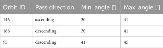
Table 2. Summary containing flight directions and range of incidence angles of each relative orbit.

The calculation of interferometric and polarimetric features necessitated the use of Single Look Complex (SLC) data (ESA, 2013). The data pre-processing involved a combined approach utilizing pyroSAR (Truckenbrodt et al., 2019), a Python-based API, and SNAP (Version 9) (ESA, 2025). This processing framework was seamlessly integrated into an ODC environment, which served as the data management platform. This platform runs on a cluster located at the Leibniz-DataCentre (LRZ) and is equipped with sufficient computation power to process at tile of SLC data in a few minutes (Friedrich et al., 2024). The polarimetric feature processing sequence comprised terrain flattening (Small, 2011), multi-looking with one look in azimuth and four looks in range, speckle filtering through a 5 pixel x 5 pixel boxcar filter, and Range-Doppler Terrain correction (Richards, 2009), yielding a spatial resolution of 20 m × 20 m and gamma nought (GN) backscatter. Given the dB scaling of backscatter, the cross-pol ratio (CR) was computed as VV-VH. Alpha and Entropy were derived from a C-2 Matrix (Cloude and Pottier, 1996). This set of S1 features consisting of VV/VH backscatter, CR, Alpha and Entropy as well as VV/VH coherence, has been proven to reflect the changes in plant physiognomy along the crop life cycle by various studies. No further decomposition metrics were included, because they possess less explanatory power in the dual-pol data of S1 when compared to quad-pol data from e.g., Radarsat. (Harfenmeister et al., 2021b; Khabbazan et al., 2019; Löw et al., 2021; Meroni et al., 2021; Schlund and Erasmi, 2020).

For interferometric (InSAR) coherence, the parameters for multi-looking and terrain correction remained consistent. Coherence calculation involved removing the flat earth and topographical phase using a moving window of three pixels in azimuth and eleven pixels in range, along with a six-day temporal baseline and consecutive reference images (Zhang et al., 2018). SRTM data (1 Arc-second) served as the digital elevation model in all steps requiring it. This set of S1 features, comprising VV/VH backscatter, CR, Alpha, and Entropy, as well as VV/VH coherence, demonstrated its ability (Harfenmeister et al., 2021a; Khabbazan et al., 2019; Löw et al., 2024; Schlund and Erasmi, 2020) to effectively capture changes in plant physiognomy related to phenological developments in various studies.

2.4 Auxiliary data

Since this study also investigated potential explanations of the spatiotemporal distribution of average agreement (AVA), dominance of tendencies (DoT) and outlier occurrences, auxiliary data was acquired and processed. The collected data represents various environmental factors that may explain the occurrence of these metrics. In regard to soil properties SoilGrid (Poggio et al., 2021) data on soil organic content (SOC), organic carbon stock (OCS) and the dominant soil type was downloaded for the area. SOC and OCS are used as proxy for soil fertility in this study. It is assumed that plants display a different physiognomy depending on the fertility of the soil. Because SAR based phenology is sensitive to changes in plant physiognomy SOC and OCS have an indirect impact on the interaction of signal and plant physiognomy. Furthermore, SOC and OCS are related to soil texture and therefore surface roughness, which is also an influencing factor in early phenological stages, when there is still soil signal present (Santos et al., 2023). In addition, daily sums of precipitation and mean air temperature were calculated from the same interpolated dataset that was used to calculate GDD (Haßelbusch and Lucas-Mofat, 2021) to support the discussion of the results in terms of local water availability. Moreover, terrain features such as aspect, slope as well as the topographical wetness index (TWI) (Sørensen et al., 2006) were derived from an SRTM30 digital elevation model. These features plus the elevation were used to explain distributions by the terrain itself. Lastly, pixel-based, mean standard deviation of yearly time series of enhanced vegetation Index (EVI) and normalized difference vegetation index (NDVI) were used as explanatory variables representing vegetation dynamics and field heterogeneity (Gessner et al., 2023). Both Indices were calculated using Sentinel-2 L2A data that were cloud-masked by the scene classification layer (SCL).

2.5 Conceptual workflow of the study

The idea behind the following approach is a comparison of various time windows. For example: In 2020, at landscape level, the TSM distribution of VH intensity of canola level displayed many relevant TSM occurrences around day of year (DOY) 115. By analysing single fields it can now be ascertained which canola fields show a similar behaviour to that pattern observed at the landscape scale. Due to the GDD baseline and distances between associated GDD values the similarity or the lack of it can be quantified. Similarly, these findings were linked to the in situ observations made by DWD. This process is applied to each S1 feature, orbit and for every year that is covered by the catalogue of Löw et al. (2024).

2.5.1 Landscape pattern of vegetation development and derivation of time windows

The approach by Löw et al. (2024) established time windows of likely phenological changes by analysing the occurrence of time series metrics (TSM), namely break points (Verbesselt et al., 2012; 2010) and extrema, across the investigative dimensions of three relative orbits, 5 years, and seven S1 features. The approach focused mainly on winter wheat, canola, sugar beet, which are also investigated by the study at hand. In response to the varying availability of in situ data a baseline of GDD was established for validation. As a result, crop specific sets of S1 features and relative orbits were identified, which provided the most accurate information on a range of phenological stadia at landscape level. Because break points outperformed extrema (Löw et al. (2024), the catalogue of this study encompasses only TSM occurrences of break points. The crop specific feature sets are listed in Table 3.

Table 3

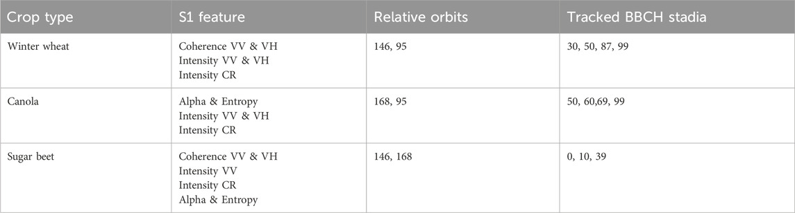
Table 3. Favourable orbits and S1 features per crop type for tracking targeted stages by break points according to the findings of Löw et al. (2024).

At first, a thresholding approach was used to identify relevant time windows within the phenological time series. These distributions are represented by TSM occurrence plots, characterised by bin sizes of 6 days and 50 GDD. Hence, a threshold of 6 days, akin to the S1 re-visitation rate, was applied to segment individual time windows associated to relevant TSM occurrences and their respective GDD distribution (see Figure 2: L1 &L2). To define these time windows in which phenological changes occur within a landscape, a k-means clustering algorithm from SciPy (Virtanen et al., 2020) was employed. Thereby, the temporal distribution of TSM occurrences was clustered using the selected S1 feature set (Table 3). The number of clusters (k_or_guess) corresponds to the number of time windows identified by the threshold approach, other parameters were left at their default value: iterations = 20, distortion threshold = 1e-05. Each time window is thus characterised by two parameters, its focal point (cluster mean) and its range (cluster radius) delineating the temporal extent of the observed phenological pattern (see Figure 2: L3 & L4). While both, thresholding and k-means yield comparable results, only k-means provides information on the distribution and the centre within a time window. Therefore, its integration was deemed necessary to enhance the characterisation of phenological patterns.

Figure 2

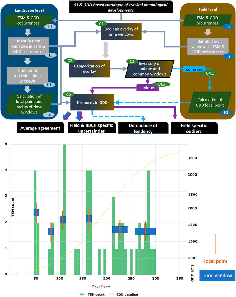
Figure 2. Top: Framework of disaggregating records at landscape level to field level and identifing common and unique time windows within the distributions of time series metrics (TSM) and Growing Degree Days (GDD), in this case break points and extrema, showcasing eachs part of the analysis and their allocation within process of disaggregating from landscape to field. Bottom: Exemplary, schematic depiction of derived time windows and their potential focal points at field level without the comparison to landscape level windows.

2.5.2 Assessing field development within the landscape pattern

At the field level, the analysis starts with a catalogue of tracked phenological developments (Table 3), their corresponding GDD values and the GDD-based distances to phenological in situ observations. The threshold-based approach described earlier is applied (see Figure 2: F1 & F2).

To evaluate the similarity between time windows at field and landscape level, a multi-step process was implemented. Firstly, a Boolean query determines whether an overlay exits (C1), i.e., whether time windows at field level (F2) intersect with those at the landscape level (L2&L4). This comparison generates an inventory of common (=overlaying) and unique time windows (C2, C3). The ‘unique’ category includes two scenarios: (i) no TSM occurrence was detected at the field level and (ii) the TSM occurrence deviates temporarily by occurring earlier or later than at landscape level For the common time windows (see Figure 2: C4.1), the focal point at field level calculated via the mean value of all values occurring within the corresponding time window at landscape level (F3). In the case of unique time windows at field level, only the distance between its border and the closest landscape time window was computed (C4.2).

2.6 Indicators of landscape-field relation

All indicators can be calculated for each year, relative orbit, S1 feature and crop type. Moreover, field specific uncertainties can be computed for each BBCH stage. Depending on the required level of detail, these indicators can be aggregated accordingly. For this study, the highest level of detail is year, crop and S1 feature specific, as the impact of relative orbits was already extensively analysed by Löw et al. (2024). Because the study at hand and Löw et al. (2024) share the same database a repetition of analyses identifying suitable combinations of relative orbits and S1 features was deemed unnecessary.

2.6.1 Average agreement

Average agreement (AVA) quantifies the representativeness of the landscape wide pattern and estimates the extent to which an individual field is aligns with that pattern. Utilizing the comparison of the TSM occurrences at field and landscape level, the average agreement (AVA) was calculated for the most relevant S1 features (Table 3). Hereby, the number of relevant, overlapping time windows at field and landscape level is computed at each field (n_field), which is, then divided by the total count of relevant time windows (N_landscape) and converted to percent (see Formula 2).

$AVA=\frac{n_{field}}{N_{landscape}}x100(2)$

A threshold of >70% was established to determine whether a field displays good agreement. This threshold was deduced from findings of Lobert et al. (2023), who showed, that the temporal onset of phenological stages in winter wheat often follows a Gaussian distribution. Hence, the threshold of 70% is derived from a rounded version of the 68% percent of data points that fall within one standard deviation. This indicator can be calculated at various levels of detail. In this study, the most detailed calculation was performed for each year and each S1 feature across all favourable orbits enabling S1 feature specific insights into the representativeness of the landscape level pattern.

2.6.2 Field & BBCH specific uncertainties

Field specific uncertainties were described by the trackable phenological progress and tracking range at field level. These serves as indicators about the variance of the TSM occurrences at field level and contributes to the quantifying uncertainties within remote sensing-based monitoring frameworks (Atzberger, 2013; Wu et al., 2023). The foundation of these uncertainty indicators is the GDD progression (GDD prog_x) described in Formula 3.

${GDDprog}_x=\frac{{GDD}_x}{{avg.GDD}_{obs}}x100(3)$

GDD prog_x towards an observation target (x) is defined as the ratio between the corresponding GDD value of the observation target (GDD_x) and the mean GDD value at landscape level (avg. GDD_obs.) across the observation period. In the context of this study, the target represents either focal points of time windows, the respective GDD value of an in situ BBCH observation or a difference between two GDD values (e.g., distance between focal points at landscape and field level).

By applying this “normalisation” similar to the crop maturity proposed by McNairn et al. (2018), a measure of vegetation development towards a targeted BBCH stage can be provided or the distance between two focal points at landscape and field level can be quantified in relative terms. As indicated by the definition of x as target, the GDD progression serves not only as foundation for field specific uncertainties, but also plays a crucial role in identifying outliers (see chapter 2.6.4).

Trackable progress and tracking range were analysed across the investigative dimensions of year, S1 features, crop type and BBCH stage. Field-specific time windows were examined within the range of 80%–120% GDD progression towards the targeted BBCH stage (e.g., BBCH 30 for winter wheat). These thresholds were established to define proximity to the target BBCH stage. This approach allowed for identifying, the closest minimum of the trackable progression for each field, indicating the earliest point at which phenological development could be observed for each field. Additionally, by calculating the maximum trackable progression, the full range of trackable progress was determined. Indicators of uncertainty were then derived for each BBCH stage covered by the in situ data as well as for each crop and S1 features across multiple orbits. These uncertainty indicators can be transformed into quality masks, when supplying information on phenological developments to stake holders. The BBCH stage serves as a bridge between a purely data driven approach and a praxis- oriented perspective. To ascertain the general plausibility of these developments field-based timelines of daily precipitation sums, average air temperature, mean EVI and the corresponding TSM occurrence plots were visually examined for coinciding trends and pattern.

2.6.3 Dominance of tendency

Dominance of tendency (DoT) quantifies the overlap of time windows between the field and landscape. The GDD distance between focal points at these two levels (see Figure 2: C5) was used to assess, whether a field was phenologically ahead or behind the broader landscape development. Additionally, it provided an indication of the magnitude of this tendency. By subtracting the field value from the landscape value negative offsets indicated a greater accumulation of GDD at the field level, implying that the field was ahead of the landscape-wide development–and vice versa. To analyse these tendencies, the number of positive and negative offsets was counted and the dominant count (n_dom) for each field across years (y) and/or S1 features (s1) was determined. This value was then normalised by the total number of landscape vs. field comparisons (N_comp), enabling a spatial assessment of general tendencies across the landscape. Analysts can hereby choose whether orbit or S1 feature specific information or only general behaviour is of interest. To demonstrate this flexibility, both the average yearly DoT across all features and a yearly, S1 specific indicator were computed. To further investigate the consistency of these tendencies the indicator was calculated as a percentage of the dominating (simple majority) tendency (see Formula 4). The results were then categorised by a query of simple majority of the dominant distances, defining three categories: ahead (dominant positive distances), behind (dominant negative distances) and equal (no dominance).

${DoT}_{y,s1}=\frac{n_{{dom}_{y,s1}}}{N_{{comp}_{y,s1}}}x100(4)$

The yearly, S1-feature specific distributions of DoT were analysed to assess how well the time windows at landscape level represent the field specific TSM occurrences. Hereby, a potential skewness of distribution within the landscape pattern could be identified in relation to S1 feature and year. Depending on the overall distribution of the predefined categories, the indicator can also be used to identify fields that exhibit a predominant phenological development ahead or behind the landscape wide trend.

2.6.4 Outliers at field level

To identify outliers that deviated from both, the overall landscape development and the BBCH stages recorded by in situ data, a two-step process was implemented. Initially, the outliers at field level were detected based on the distance between borders of time windows at landscape level and unique time windows at field level (see Figure 2: C5). This distance was then evaluated using a GDD based threshold to determine whether a unique time window truly qualified as an outlier. A time window was classified as an outlier, if the distance between borders is greater than 15 GDD. 15 GDD was identified as value that represents one to 2 days of GDD accumulation in average growing conditions for each of the investigated crop type. In a second step, these outliers were cross-referenced with the in situ observation of BBCH stages using GDD progression. After thresholding, additional filtering was applied based on the GDD-based progress towards BBCH stages. Only outliers with a progression between 25% and 70% and exceeding 130% were considered. By counting the occurrences of these outliers across the entire observation period as well as across all crop types and S1 features, fields that are likely to diverge from the landscape-wide phenological patterns were identified. Aggregating this information across multiple years, crops, orbits and S1 features allows for the detection of deviation hot spots. The identification of such hot spots can provide insight into either uncommon management practices (Stobbelaar et al., 2004) or increased susceptibility to stressors (Ajadi et al., 2020; Singh et al., 2007) associated with adverse geographic conditions.

2.7 Checking the plausibility of an indicator’s spatial distribution

Subsequently, a conceptual approach was developed that assesses the spatial distribution of the above listed indicators. This assessment addresses the explainability of said indicators via the geographical settings of the study area. In an exemplary analysis, the plausibility of outliers at field level were investigated via Spearman’s rank correlation coefficient and the variable importance of a random forest (Breiman, 2001; Conrad et al., 2017). It was hypothesized that deviations at the field level from the landscape pattern depend on the field-specific environmental conditions. Hereby, a variety of environmental descriptors were included. An exemplary set of indicators is illustrated in Figure 3. The full list and the corresponding abbreviations are listed in the Supplementary Appendix (see Supplementary Table SA1). Matching pairs for the correlation analysis and training the random forest were extracted as mean values per field, except for soil type, where the dominant class was derived by modus.

Figure 3

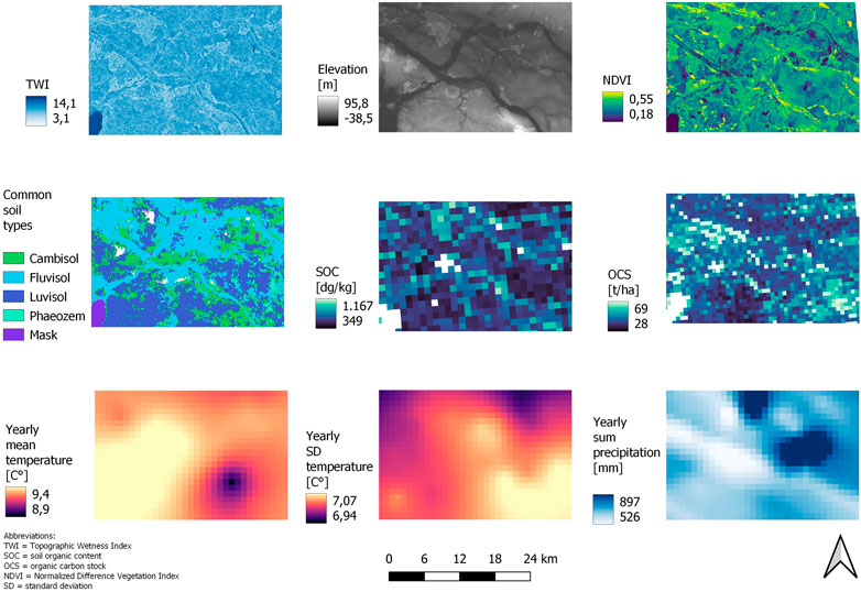
Figure 3. Exemplary list of spatial indicators containing terrain (TWI, elevation above ellipsoid), vegetation (NDVI), soil (OCS, SOC, common soil type) and weather (temperature, precipitation) features.

The internal model accuracy of the various random forests was evaluated using root mean square error (RMSE, mean absolute error (MAE) and R squared. These metrics were derived by the internal accuracy assessment provided by the R package caret (Kuhn, 2008).

3 Results

3.1 Average agreement (AVA)

Figure 4 presents an example of field specific information on winter wheat across the years 2017, 2018, 2020 and 2021, illustrating the mean agreement across all relevant S1 features. The substantial proportion of fields exhibiting an AVA below 40% in 2017 and 2021 reflects the findings of the yearly, S1 feature specific analysis (see below). However, the majority of fields across all years were allocated within the 50%–80% agreement range. Also, fields of higher rates of agreement were detected in the south eastern, south western and north eastern region across all depicted years. Notably, fields exceeding 90% of AVA concentrated in 2020, suggesting a greater homogeneity in crop development. According to yearly, S1 feature specific statistics, winter wheat exhibited comparatively low rates of agreement, particularly for VV and VH intensity in the years of 2017 (40%) and 2021 (60%). While canola displayed a similar gradient when comparing VV and VH intensities with other S1 features, the yearly performance is lowest in 2018 and 2019 Nevertheless, canola’s overall the agreement rate is greater than winter wheat, but lower than sugar beet. In contrast, sugar beet consistently achieved the highest agreement rates, exceeding 85%, whereas canola and winter wheat mainly ranged around 70%.

Figure 4

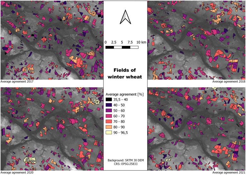
Figure 4. Example of field specifc rate of average agreement in % covering fields of winter wheat in 2017, 2018, 2020 and 2021. Values close to 100% indicate a strong agreement with the overall development at landscape level, whereas low values suggest either the absence of common time windows or an increased number of deviations. Such information provides a spatial measure for the representativity of the landscape wide pattern.

As shown in Equation 3, the information on AVA was initially derived for each year and S1 feature. This provided spatially explicit information on the extent to which each field aligns with the TSM and GDD occurrences at landscape level.

3.2 Field & BBCH specific uncertainties and their plausibility

The trackable progress was calculated for each BBCH stage, relevant S1 feature and year within the observation period. This resulted in large quantities of vector data, exceeding the scope of this paper for comprehensive presentation. Therefore, Figure 5 only displays an exemplary data set derived from VV coherence for wheat fields in 2017.

Figure 5

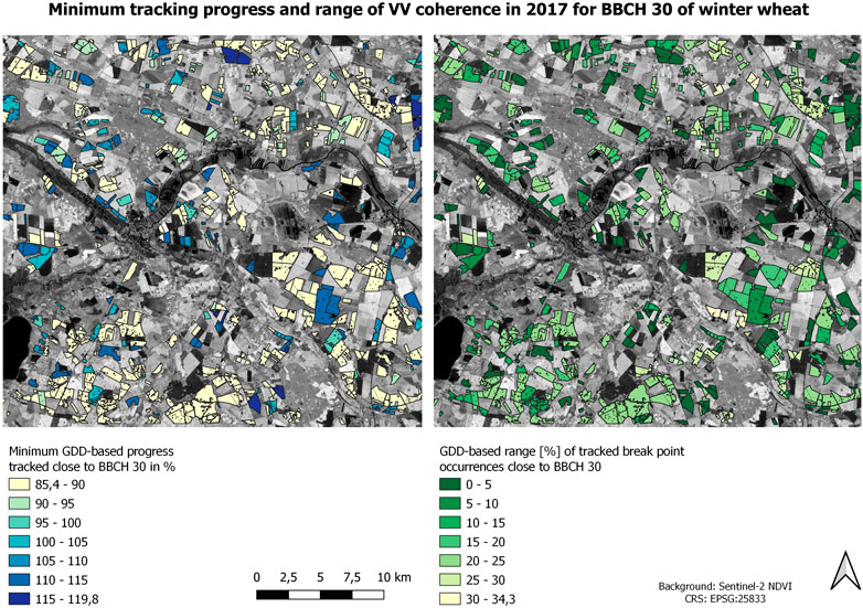
Figure 5. Left: Minimum of trackable progress in GDD progression close (80%–120%) to BBCH 30 (stem elongation) for winter wheat by VV coherence in 2017. Lower values suggest an earlier detection. Right: Corresponding range of tracked GDD-based progress. Low values inidcate a comparatively precise tracking result, whereas high numbers suggest that the tracked BBCH stage displayed a greater temporal variance. providing a quality mask for tracking results.

The left panel of Figure 5 illustrates the minimum tracking progress of GDD coinciding with the first relevant TSM occurrence in the S1 signal. The large number of fields fall within the range of 85%–90%, which is congruent with the DoT findings, where most winter wheat fields exhibit advanced development relative to the time window at landscape level. However, a subset of fields falls within the range of 110%–115%, indicating later development. The right panel of Figure 5 displays the range of GDD-based progression covered by TSM occurrences. In this example, the fewest fields were observed within the range of 30%–34.5%.

By plotting the field and BBCH specific tracking range for the same S1 feature across multiple years (see Figure 6), it became evident that there is a notable variance in the distribution of values. The years 2017 and 2021 depict a higher number of fields within larger ranges (20%–35%) whereas 2018 and especially 2019 were dominated by fields with lower ranges (0%–10%). Furthermore, distinct spatial cluster of consistently high or low ranges could be identified.

Figure 6

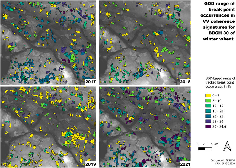
Figure 6. Exemplary range of trackable progress close (80%–120%) to BBCH 30 (stem elongation) for winter wheat by VV coherence for the years 2017, 2018, 2019 and 2021. Low values inidcate a comparatively precise tracking result, whereas high numbers suggest that the tracked BBCH stage displayed a greater temporal variance.

By inspecting an exemplary field specific timeline (see Figure 7), a semi-regular pattern emerged. Relevant occurrences of break points were tracked for the selected field around Julian Days 50, 100 to 125 and 175 to 225. Additionally, the distribution of TSM occurrences appeared more compact in years with higher rainfall intensities, which aligns with a larger number of fields exhibiting wider tracking ranges in 2017 and 2021 (see Figure 6). Furthermore, rainfall events did not regularly overlay with the occurrences of break points. Besides, when comparing the EVI time series with the occurrences of break points, the observed patterns are mostly congruent with the overall trends depicted by the EVI time series, despite some inconsistencies in the data availability.

Figure 7

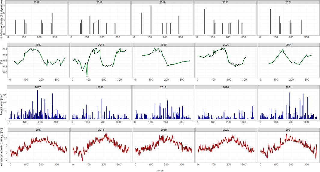
Figure 7. Exemplary time lines of a field of winter wheat for each year (2017–2021), showcasing the occurrences of break points in VV coherence derived from orbit 95 as well as the temporal signatures of EVI, their daily sum of precipitation and their daily mean air temperature.

3.3 Dominance of tendency (DoT)

At field level, detailed information about DoT and its spatial distribution is displayed (see Figure 8). The distribution of time windows appears skewed, which is in line with the findings observed at the landscape scale, which are described in a subsequent paragraph. Furthermore, information on the strength of the DoT was illustrated. In 2017 (see Figure 8), for example, sugar beet predominantly depicts fields of strong positive consistencies, whereas in 2020 and 2021 a higher proportion of fields displayed negative DoT, consistent with the yearly, S1-specific observations. Similarly, the occurrences of 2018 are consistent with the dominance of negative rates in three S1 features. In this map no clear spatial clustering of DoT across multiple years was found. This contrasts the findings in the example of AVA (see Figure 4), where clusters of similar agreement rates could be found across multiple years.

Figure 8

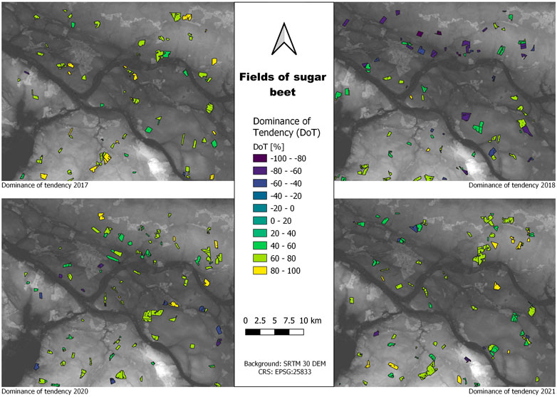
Figure 8. Example of field specifc rate of DoT in % covering fields of sugar beet in 2017, 2018, 2020 and 2021. High positive values indicate that a field is strongly ahead of the development at landscape level, whereas negative values suggesst that a field is lagging behind revealing fields that maybe subject to stressors or uncommon management practices.

The yearly, S1 feature specific analysis of DoT revealed, that most fields of winter wheat and canola (see Figure A6) display a dominant positive DoT across all S1 features and years. In contrast, sugar beet depicted a more variable pattern. For example, coherences in 2017 were mostly dominated by the equal category. In 2018, the behind category was dominant for Alpha, Entropy and CR, whereas similar distributions of categories were observed only for VH coherence and VV intensity in 2019.

3.4 Outliers at field level and their plausibility

The analysis of deviations and outliers revealed that the individual field deviated from the landscape pattern up to 200 times (see Figure 9). However, these numbers reflect the total count across all observed years, crop types, S1 features, and relative orbits. By examining Figure 9, it becomes evident, that the majority of fields displays between 20 and 80 outliers. Higher outlier counts (above 120) are mostly concentrated within a few spatial clusters, particularly in the North-Northeast and the Southwestern part of the study area.

Figure 9

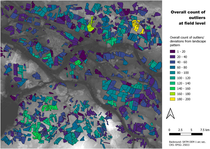
Figure 9. Field specific count of deviations from the landscape level patterns (outliers). High values indicate larger numbers of deviations from landscape level pattern flagging fields for closer inspections in regard to stress or management anomalies.

As addressed in chapter 2.7, an analysis of potential environmental explanations was conducted. The correlation analysis yielded weak, but significant (p = 0.05) correlation coefficients for the following variables elevation (elev_mean; 0.26), dominant soil type (soil_type 0.26), soil organic content at 0–5 cm (soc_mean; −0.23) and organic carbon stock at 0–30 cm (ocs_mean; −0.23). These results are visualised in Figure 10. The strongest correlation was found between organic carbon stock (ocs_mean) and elevation (elev_mean) (−0.45).

Figure 10

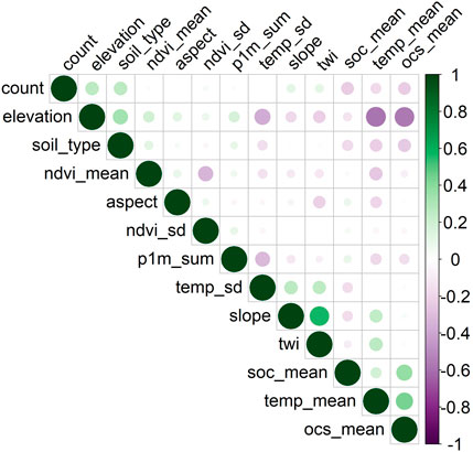
Figure 10. Correlation plot (Spearman’s r) of environmental variables for describing number of deviations from landscape patterns. Lables in Supplementary Table SA1.

In accordance with the correlation analysis, the variable importance of the random forest revealed elevation as the most important predictor of the total outlier count. The second and third most important variables were organic carbon stock at 0–30 cm (ocs_mean) and soil organic carbon content at 0–5 cm (soc_mean) (Figure 11).

Figure 11

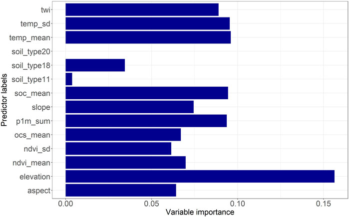
Figure 11. Variable importance of rf explaining the spatial distribution of overall outliers. Numbers of soil_majority refer to the soil class according to soil grids data base: 11 = Fluvisol, 18 = Luvisol, 20 = Phaeozems. Higher values indicate an increased importance.

The accuracy assessment yielded the following results: RMSE = 33.5, MAE = 26.2 and R² = 0.25. Additionally, the crop specific analysis of outlier occurrences and deviations from the landscape pattern provided the following insights, summarised in Table 4.

Table 4

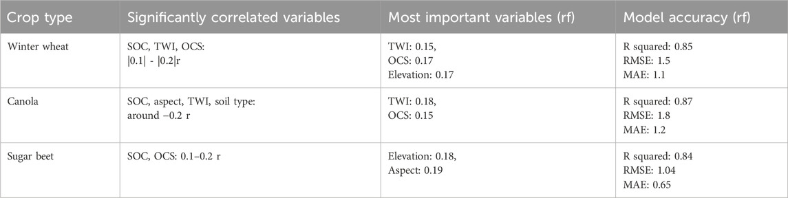
Table 4. Results of crop specific correlation analysis (Spearman’s r) and variable importance to explain deviations from landscape pattern/outlier occurrences.

The model accuracy for all three crop types was consistent with values around 0.85. Soil organic carbon content (SOC) exhibited a weak correlation with the outlier occurrences of all crop types. Furthermore, terrain features such as elevation and TWI were ranked as the variables of highest importance.

4 Discussion

The approach presented here effectively links SAR-based landscape wide vegetation pattern to field specific phenological developments. The linkage addresses two key questions: (i) the agreement between the signal developments at both levels, and (ii) the detection of temporal offsets and outliers at the field level. Such cross-scale comparisons are rare in time series-based approaches, which mostly compare estimates with in situ observation using temporal distance (Harfenmeister et al., 2021a; Lobert et al., 2023; Schlund and Erasmi, 2020). Furthermore, uncertainties within in situ data are seldom quantified. For instance, the phenological observations within the DWD monitoring framework are reported, when 50% of a field has reached a specific stage. Hereby, the recommended re-visitation rate is two to three times per week. These issues alone introduce two sources of uncertainties when ascertaining phenological stages of a field. By providing relational and relative indicators, i.e., trackable progress and average agreement, these uncertainties were captured and quantified. This was achieved by adapting the concept of crop maturity (McNairn et al., 2018) to generate a GDD based progression towards stages of interest. Moreover, the relational nature and the integration of a baseline decrease the need for extensive in situ data collection and make the study’s methods transferable to other geographical contexts, where the development or performance of individual landscape elements in relation to broader patterns is essential. Potential transfer applications are listed in the conclusion. The subsequent chapters address implications, the potential and limitations of this study.

4.1 Discussing average agreement and DoT

The exemplary analysis of the AVA showed that fields tend to agree with the overall pattern at landscape level between 60% and 70%. Hence it is assumed that the predefined threshold of 70% is valid for designating fields or in a wider context also years and S1 features of high agreement. Moreover, the indicator demonstrated its potential to serve as measurement of how well a S1 feature is able to reflect heterogeneous developments within a landscape. Because S1 features that produce high rates of averages agreement are most likely less sensitive towards field specific developments.

The calculation and field specific visualization of DoT revealed that the majority of depicted fields tended to be ahead of the landscape. Because this study relied on phenological statistics at the state level such bias was expected. Nevertheless, DoT showcases the potential of the landscape-field comparison, as it produces information on growth progress by incorporating multiple S1 features and orbits without the explicit need of in situ data. Because AVA and DoT derive their explanatory power mainly from deviations between field and landscape level time windows instead of in situ observation the impact of biases introduced by point to pixel mismatches inherent to DWD data was mitigated.

When combining DoT with the rate of agreement, flags or labels can be created for fields that exhibit strong negative tendencies and low AVA. Such flags might prove useful for investigating landscapes in terms of their climate vulnerability, resilience or differences in management practice, especially when agents, such as policymakers or consultants who may lack local knowledge are involved. Furthermore, these flags can serve as an initial indicator for pinpointing areas to start ground surveys on crop damage induced by extreme weather events, outbreaks of diseases or pest infestation (Ajadi et al., 2020; Singh et al., 2007; Stobbelaar et al., 2004).

4.2 Outliers, deviations and trackability

During the explanatory analysis of outliers and deviations across multiple years and crop types, no single, dominant descriptor was identified. The crop specific analysis yielded a slightly stronger emphasis on TWI and OCS/SOC instead of raw elevation. However, as previously mentioned, no dominant descriptor emerged, further supporting the indication of a complex system behind the spatial and temporal occurrence of time windows. Despite this complexity, the model accuracy as indicated by MAE and RMSE (around one to two outlier occurrences) suggests a high prediction potential when combining all environmental descriptors. From a data perspective, it seems logical that these descriptors ranked highly in most explanatory analyses, given that terrain (Yang et al., 2011), soil organic carbon (Santos et al., 2023) and wetness or moisture (Esch, 2018; Pichierri et al., 2018) have well documented impacts on SAR signals. However, their impact on phenological development is highly dependent on the phenological stage and crop type (Canisius et al., 2018).

The GDD-based range of trackability (see chapter 2.6.4) and the initial uptake of signal change provided a different perspective on the accuracy of time series-based monitoring, especially when describing uncertainties. Considering the complexity of S1 time series (with varying viewing geometries, different smoothing algorithms and length of time series) (Harfenmeister et al., 2021b; Löw et al., 2024; Meroni et al., 2021; Qadir et al., 2023), such a measure can be converted to a quality mask at the field level. As mentioned earlier in of the discussion, in situ observations of phenological development are rarely a binary issue. Therefore, a range of uncertainties seems more appropriate for describing the semi-continuous (Meier, 2001) process of crop development, rather than simple temporal differences. However, constant and extensive monitoring of landscapes and their phenological development may improve overall tracking capabilities (d’Andrimont et al., 2022; Tran et al., 2022). Interestingly, the exemplary time line of tracking ranges (see Figure 6) indicate, that drier years produce smaller tracking ranges and thus more accurate predictions. This contrasts with the findings of Schlund and Erasmi (2020), who concluded that tracking quality of InSAR coherence decreases during years of drought. It is however important to note that Schlund and Erasmi (2020) conducted a single orbit study while the present study combined orbits 95 and 146 for winter wheat. Therefore, it is assumed that the effect of different viewing geometries on InSAR coherence result in a larger tracking range within a multi-orbit framework.

Compared to AVA and DoT, the tracking range and trackability are more dependent on the availability of phenological in situ observations. But this study demonstrated that statistics at the level of federal state already provide sufficient information to calibrate the ranges, thanks to the attached GDD baseline and its translation into phenological progress. Hence the point to pixel mismatch within the DWD data is also considered of minor importance.

5 Conclusion and outlook

This study introduced a novel approach to tracking phenological developments employing S1 time series and capturing the underlying uncertainties. To that end, a relational framework between the landscape-level and field-specific development was established. The concept of time windows related to phenological changes was applied to generate the following insights:

• Indicator of AVA. It provides a general estimate of how well the phenological development at field level is represented by the patterns at landscape level. Additionally, it quantifies the representativeness of the landscape pattern.

• DoT: This indicator reveals whether a field is ahead or behind the general phenological development at the landscape level and assesses how dominant that tendency is.

• Field specific outliers. This measures how often a field disagrees with or deviates from the landscape pattern, which compliments the information provided by AVA.

Furthermore, spatially explicit information was generated on how early phenological development can be tracked alongside the range of trackable progress. This information can now be converted into a quality mask by applying crop and stage specific thresholds to the range. Additionally, this framework identified environmental descriptors, which by tendency were found to explain the temporal and spatial distribution of the above listed data. A relational and contextual framework was thus developed, capable of capturing and describing varieties and uncertainties within the landscape, without relying on large amounts of field specific and time accurate in situ observations.

This framework heavily depends on the availability of information on field boundaries and crop inventories. Additional information on crop management strategies would further enhance the explanatory power of this analysis. To address these challenges the Earth observation community has already been developing solutions to provide such data products (Blickensdörfer et al., 2022; Orynbaikyzy et al., 2022; Tetteh et al., 2020).

This study as along with others demonstrated that temporal SAR signatures, either on their own or combined with GDD, are capable of reflecting crop development. Hence, subsequent research can now investigate the scalability of this framework to the state or nation level. In that process, different crop rotations should not necessarily affect the scalability, because the approach is built around time windows of relevant signal change which should occur in any cropping system and can subsequently be related to crop phenology via GDD. The fragmentation of a landscape considered more challenging due to the influence of mixed pixel issues introduced by small field sizes and intercropping. Therefore, different sensors of higher spatial resolution such as TerraSAR/TanDEM-X could be an option. Alternatively, the transferability of such an approach to other regions, different types of vegetation (e.g., forest) or other phenological cycles, such as snow and ice phenology could also be of interest. Given the computation and processing steps of this framework, it is not feasible to transfer it as is to a near real time framework. However, this study, like others before has demonstrated that the shapes of S1 time series are able to reflect phenological progress. Due to the enhanced processing capabilities of cloud computing the analysis and comparison of similarities between the shapes of time series seems to be possible in a near real time framework Hence, future research could assess, how a measure of similarity between past and recent time series can be used to move from tracking developments of past seasons to assessing crop performance in a near real time framework. By linking field boundaries to unique identifiers, any data or records on yield, stress or resource requirements of a field and season that were deemed most similar, could now be utilized in a data driven management strategy by farmers or other actors in the agricultural domain.

Data availability statement

The data analyzed in this study is subject to the following licenses/restrictions: The data on field boundaries and crop types of the land parcel identification system was used under a third party agreement, that prohibits sharing with third parties not directly linked to the research project. Requests to access these datasets should be directed to am9oYW5uZXMubG9ld0BnZW8udW5pLWhhbGxlLmRl.

Author contributions

JL: Conceptualization, Validation, Methodology, Data curation, Writing – review and editing, Resources, Writing – original draft, Formal Analysis, Software, Visualization, Investigation. SH: Data curation, Writing – review and editing, Software. IO: Supervision, Writing – review and editing, Project administration. CF: Writing – review and editing, Data curation, Software. MT: Funding acquisition, Writing – review and editing, Resources, Project administration. TU: Supervision, Writing – review and editing, Conceptualization. CC: Resources, Project administration, Writing – review and editing, Funding acquisition, Supervision.

Funding

The author(s) declare that financial support was received for the research and/or publication of this article. This research was funded by German Aerospace Center (PhenoSAR: Demmin: FKZ: 0067286236), Martin-Luther-University of Halle-Wittenberg, as well as the German Ministry of Agriculture via the project of AgriSens Demmin 4.0 (FKZ: 28DE114E18). It was also funded by The German Ministry of Education and Research via the project DIP-ZAZIkI (FKZ: 031B1460B).

Acknowledgments

We would like to thank ESA for providing open access to Sentinel-1 data as well as our project partners for supplying the data on field boundaries and crop types.

Conflict of interest

The authors declare that the research was conducted in the absence of any commercial or financial relationships that could be construed as a potential conflict of interest.

Generative AI statement

The author(s) declare that Generative AI was used in the creation of this manuscript. During the preparation of this work the author(s) used perplexity AI in order to increase conciseness and improve readability of the abstract and introduction. After using this tool/service, the author(s) reviewed and edited the content as needed and take(s) full responsibility for the content of the published article.

Any alternative text (alt text) provided alongside figures in this article has been generated by Frontiers with the support of artificial intelligence and reasonable efforts have been made to ensure accuracy, including review by the authors wherever possible. If you identify any issues, please contact us.

Publisher’s note

All claims expressed in this article are solely those of the authors and do not necessarily represent those of their affiliated organizations, or those of the publisher, the editors and the reviewers. Any product that may be evaluated in this article, or claim that may be made by its manufacturer, is not guaranteed or endorsed by the publisher.

Supplementary material

The Supplementary Material for this article can be found online at: https://www.frontiersin.org/articles/10.3389/frsen.2025.1610005/full#supplementary-material

References

Ajadi, O. A., Liao, H., Jaacks, J., Delos Santos, A., Kumpatla, S. P., Patel, R., et al. (2020). Landscape-scale crop lodging assessment across Iowa and Illinois using synthetic aperture radar (SAR) images. Remote Sens. (Basel) 12, 3885. doi:10.3390/rs12233885

CrossRef Full Text | Google Scholar

Arias, M., Campo-Bescós, M. Á., and Álvarez-Mozos, J. (2022). On the influence of acquisition geometry in backscatter time series over wheat. Int. J. Appl. Earth Observation Geoinformation 106, 102671. doi:10.1016/j.jag.2021.102671

CrossRef Full Text | Google Scholar

Atzberger, C. (2013). Advances in remote sensing of agriculture: context description, existing operational monitoring systems and major information needs. Remote Sens. (Basel) 5, 949–981. doi:10.3390/rs5020949

CrossRef Full Text | Google Scholar

Blickensdörfer, L., Schwieder, M., Pflugmacher, D., Nendel, C., Erasmi, S., and Hostert, P. (2022). Mapping of crop types and crop sequences with combined time series of Sentinel-1, Sentinel-2 and landsat 8 data for Germany. Remote Sens. Environ. 269, 112831. doi:10.1016/j.rse.2021.112831

CrossRef Full Text | Google Scholar

Breiman, L. (2001). Random forests. Mach. Learn 45, 5–32. doi:10.1023/A:1010933404324

CrossRef Full Text | Google Scholar

Canisius, F., Shang, J., Liu, J., Huang, X., Ma, B., Jiao, X., et al. (2018). Tracking crop phenological development using multi-temporal polarimetric Radarsat-2 data. Remote Sens. Environ. 210, 508–518. doi:10.1016/j.rse.2017.07.031

CrossRef Full Text | Google Scholar

Cloude, S. R., and Pottier, E. (1996). A review of target decomposition theorems in radar polarimetry. IEEE Trans. Geoscience Remote Sens. 34, 498–518. doi:10.1109/36.485127

CrossRef Full Text | Google Scholar

Conrad, C., Löw, F., and Lamers, J. P. A. (2017). Mapping and assessing crop diversity in the irrigated Fergana valley, Uzbekistan. Appl. Geogr. 86, 102–117. doi:10.1016/j.apgeog.2017.06.016

CrossRef Full Text | Google Scholar

Derakhshan, A., Bakhshandeh, A., Siadat, S.A., Moradi-Telavat, M. R., and Andarzian, S. B. (2018). Quantifying the germination response of spring canola (Brassica napus L.) to temperature. Ind. Crops Prod. 122, 195–201. doi:10.1016/j.indcrop.2018.05.075

CrossRef Full Text | Google Scholar

d’Andrimont, R., Taymans, M., Lemoine, G., Ceglar, A., Yordanov, M., and van der Velde, M. (2020). Detecting flowering phenology in oil seed rape parcels with Sentinel-1 and -2 time series. Remote Sens. Environ. 239, 111660. doi:10.1016/j.rse.2020.111660

PubMed Abstract | CrossRef Full Text | Google Scholar

d’Andrimont, R., Yordanov, M., Martinez-Sanchez, L., and van der Velde, M. (2022). Monitoring crop phenology with street-level imagery using computer vision. Comput. Electron Agric. 196, 106866. doi:10.1016/j.compag.2022.106866

CrossRef Full Text | Google Scholar

ESA (2013). Sentinel-1 user handbook.

Google Scholar

ESA (2025). STEP – science toolbox exploitation platform. Available online at: https://step.esa.int/main/(Accessed July 1, 2025).

Google Scholar

Esch, S. (2018). Determination of soil moisture and vegetation parameters from spaceborne C-Band SAR on agricultural areas.

Google Scholar

Friedrich, C., Löw, J., Otte, I., Hill, S., Förtsch, S., Schwalb-Willmann, J., et al. (2024). “A multi-talented datacube: integrating, processing and presenting big geodata for the agricultural end user,” in Informatik in Der Land-, Forst Und Ernährungswirtschaft. Fokus: Biodiversität Fördern Durch Digitale Landwirtschaft. Editors C. Hoffmann, A. Stein, E. Gallmann, J. Dörr, C. Krupitzer, and H. Floto (Hohenheim-Stuttgart), 251–256.

Google Scholar

Gessner, U., Reinermann, S., Asam, S., and Kuenzer, C. (2023). Vegetation stress monitor—assessment of drought and temperature-related effects on vegetation in Germany analyzing MODIS time series over 23 years. Remote Sens. (Basel) 15, 5428. doi:10.3390/rs15225428

CrossRef Full Text | Google Scholar

Harfenmeister, K., Itzerott, S., Weltzien, C., and Spengler, D. (2021a). Agricultural monitoring using polarimetric decomposition parameters of sentinel-1 data. Remote Sens. (Basel) 13, 575–28. doi:10.3390/rs13040575

CrossRef Full Text | Google Scholar

Harfenmeister, K., Itzerott, S., Weltzien, C., and Spengler, D. (2021b). Detecting phenological development of winter wheat and winter barley using time series of Sentinel-1 and Sentinel-2. Remote Sens. (Basel) 13, 5036. doi:10.3390/rs13245036

CrossRef Full Text | Google Scholar

Haßelbusch, K., and Lucas-Mofat, A. (2021). Rasterdaten für die Agrarmeteorologie: vergleich verschiedener Interpolationsverfahren am Beispiel AgriSens Demmin 4.0. Braunschweig.

Google Scholar

Hosseini, M., McNairn, H., Mitchell, S., Robertson, L. D., Davidson, A., Ahmadian, N., et al. (2021). A comparison between support vector machine and water cloud model for estimating crop leaf area index. Remote Sens. (Basel) 13, 1348. doi:10.3390/rs13071348

CrossRef Full Text | Google Scholar

Htitiou, A., Möller, M., Riedel, T., Beyer, F., and Gerighausen, H. (2024). Towards optimising the derivation of phenological phases of different crop types over Germany using satellite image time series. Remote Sens. (Basel) 16, 3183. doi:10.3390/rs16173183

CrossRef Full Text | Google Scholar

Jacott, C. N., and Boden, S. A. (2020). Feeling the heat: developmental and molecular responses of wheat and barley to high ambient temperatures. J. Exp. Bot. 71, 5740–5751. doi:10.1093/jxb/eraa326

PubMed Abstract | CrossRef Full Text | Google Scholar

Kaspar, F., Zimmermann, K., and Polte-Rudolf, C. (2015). An overview of the phenological observation network and the phenological database of Germany’s national meteorological service (deutscher wetterdienst). Adv. Sci. Res. 11, 93–99. doi:10.5194/asr-11-93-2014

CrossRef Full Text | Google Scholar

Khabbazan, S., Vermunt, P., Steele-Dunne, S., Arntz, L. R., Marinetti, C., van der Valk, D., et al. (2019). Crop monitoring using Sentinel-1 data: a case study from the Netherlands. Remote Sens. (Basel) 11, 1887–24. doi:10.3390/rs11161887

CrossRef Full Text | Google Scholar

Killough, B. (2018). “Overview of the open data cube initiative,” in International geoscience and remote sensing symposium (IGARSS) (Institute of Electrical and Electronics Engineers Inc.), 8629–8632. doi:10.1109/IGARSS.2018.8517694

CrossRef Full Text | Google Scholar

Kuhn, M. (2008). Building predictive models in R using the caret package. J. Stat. Softw. 28, 1–26. doi:10.18637/jss.v028.i05

PubMed Abstract | CrossRef Full Text | Google Scholar

Lobert, F., Löw, J., Schwieder, M., Gocht, A., Schlund, M., Hostert, P., et al. (2023). A deep learning approach for deriving winter wheat phenology from optical and SAR time series at field level. Remote Sens. Environ. 298, 113800. doi:10.1016/j.rse.2023.113800

CrossRef Full Text | Google Scholar

Löw, J., Ullmann, T., and Conrad, C. (2021). The impact of phenological developments on interferometric and polarimetric crop signatures derived from sentinel-1: examples from the DEMMIN study site (germany). Remote Sens. (Basel) 13, 2951. doi:10.3390/rs13152951

CrossRef Full Text | Google Scholar

Löw, J., Hill, S., Otte, I., Thiel, M., Ullmann, T., and Conrad, C. (2024). How phenology shapes crop-specific Sentinel-1 PolSAR features and InSAR coherence across multiple years and orbits. Remote Sens. (Basel) 16, 2791. doi:10.3390/rs16152791

CrossRef Full Text | Google Scholar

Mandal, D., Kumar, V., Ratha, D., Dey, S., Bhattacharya, A., Lopez-Sanchez, J. M., et al. (2020). Dual polarimetric radar vegetation index for crop growth monitoring using sentinel-1 SAR data. Remote Sens. Environ. 247, 111954. doi:10.1016/j.rse.2020.111954

CrossRef Full Text | Google Scholar

Mascolo, L., Martinez-Marin, T., and Lopez-Sanchez, J. M. (2024). A novel dynamical framework for crop phenology estimation with remote sensing. IEEE J. Sel. Top. Appl. Earth Obs. Remote Sens. 18, 2208–2225. doi:10.1109/JSTARS.2024.3516212

CrossRef Full Text | Google Scholar

McMaster, G. S., and Smika, D. E. (1988). Estimation and evaluation of winter wheat phenology in the central great plains. Agric For Meteorol 43, 1–18. doi:10.1016/0168-1923(88)90002-0

CrossRef Full Text | Google Scholar

McMaster, G. S., and Wilhelm, W. W. (1997). Growing degree-days: one equation, two interpretations. Agric For Meteorol 87, 291–300. doi:10.1016/S0168-1923(97)00027-0

CrossRef Full Text | Google Scholar

McNairn, H., Jiao, X., Pacheco, A., Sinha, A., Tan, W., and Li, Y. (2018). Estimating canola phenology using synthetic aperture radar. Remote Sens. Environ. 219, 196–205. doi:10.1016/j.rse.2018.10.012

CrossRef Full Text | Google Scholar

Meier, U. (2001). “Growth stages of mono-and dicotyledonous plants,” in BBCH monograph, 2nd ed, federal biological research centre for agriculture and forestry. Federal biological research centre for agriculture and forestry. Berlin, Braunschweig.

Google Scholar

Meroni, M., d’Andrimont, R., Vrieling, A., Fasbender, D., Lemoine, G., Rembold, F., et al. (2021). Comparing land surface phenology of major European crops as derived from SAR and multispectral data of Sentinel-1 and -2. Remote Sens. Environ. 253, 112232. doi:10.1016/j.rse.2020.112232

PubMed Abstract | CrossRef Full Text | Google Scholar

Nasrallah, A., Baghdadi, N., El Hajj, M., Darwish, T., Belhouchette, H., Faour, G., et al. (2019). Sentinel-1 data for winter wheat phenology monitoring and mapping. Remote Sens. (Basel) 11, 2228. doi:10.3390/rs11192228

CrossRef Full Text | Google Scholar

Orynbaikyzy, A., Gessner, U., and Conrad, C. (2022). Spatial transferability of random forest models for crop type classification using Sentinel-1 and Sentinel-2. Remote Sens. 14, 1493. doi:10.3390/RS14061493

CrossRef Full Text | Google Scholar

Pichierri, M., Hajnsek, I., Zwieback, S., and Rabus, B. (2018). On the potential of polarimetric SAR interferometry to characterize the biomass, moisture and structure of agricultural crops at L-C- and X-Bands. Remote Sens. Environ. 204, 596–616. doi:10.1016/j.rse.2017.09.039

CrossRef Full Text | Google Scholar

Poggio, L., De Sousa, L. M., Batjes, N. H., Heuvelink, G. B. M., Kempen, B., Ribeiro, E., et al. (2021). SoilGrids 2.0: producing soil information for the globe with quantified spatial uncertainty. SOIL 7, 217–240. doi:10.5194/soil-7-217-2021

CrossRef Full Text | Google Scholar

Povey, A. C., and Grainger, R. G. (2015). Known and unknown unknowns: uncertainty estimation in satellite remote sensing. Atmos. Meas. Tech. 8, 4699–4718. doi:10.5194/amt-8-4699-2015

CrossRef Full Text | Google Scholar

Qadir, A., Skakun, S., Eun, J., Prashnani, M., and Shumilo, L. (2023). Sentinel-1 time series data for sunflower (Helianthus annuus) phenology monitoring. Remote Sens. Environ. 295, 113689. doi:10.1016/j.rse.2023.113689

CrossRef Full Text | Google Scholar

Radke, J. K., and Bauer, R. E. (1969). Growth of sugar beets as affected by root temperatures part I: greenhouse studies ¹. Agron. J. 61, 860–863. doi:10.2134/agronj1969.00021962006100060009x

CrossRef Full Text | Google Scholar

Richards, J. A. (2009). Remote sensing with imaging radar.

Google Scholar

Ritchie, J. T., and Nesmith, D. S. (2015). “Temperature and crop development,” in Modeling plant and soil systems (Wiley Blackwell), 5–29. doi:10.2134/agronmonogr31.c2

CrossRef Full Text | Google Scholar

Sakamoto, T., Gitelson, A. A., and Arkebauer, T. J. (2013). MODIS-based corn grain yield estimation model incorporating crop phenology information. Remote Sens. Environ. 131, 215–231. doi:10.1016/j.rse.2012.12.017

CrossRef Full Text | Google Scholar

Santos, E.P. dos, Moreira, M. C., Fernandes-Filho, E. I., Demattê, J. A. M., Dionizio, E. A., Silva, D.D. da, et al. (2023). Sentinel-1 imagery used for estimation of soil organic carbon by dual-polarization SAR vegetation indices. Remote Sens. (Basel) 15, 5464. doi:10.3390/rs15235464

CrossRef Full Text | Google Scholar

Schlund, M. (2025). Potential of Sentinel-1 time-series data for monitoring the phenology of European temperate forests. ISPRS J. Photogrammetry Remote Sens. 223, 131–145. doi:10.1016/j.isprsjprs.2025.02.026

CrossRef Full Text | Google Scholar

Schlund, M., and Erasmi, S. (2020). Sentinel-1 time series data for monitoring the phenology of winter wheat. Remote Sens. Environ. 246, 111814. doi:10.1016/j.rse.2020.111814

CrossRef Full Text | Google Scholar

Singh, D., Sao, R., and Singh, K. P. (2007). A remote sensing assessment of pest infestation on sorghum. Adv. Space Res. 39, 155–163. doi:10.1016/j.asr.2006.02.025

CrossRef Full Text | Google Scholar

Small, D. (2011). Flattening gamma: radiometric terrain correction for SAR imagery. IEEE Trans. Geoscience Remote Sens. 49, 3081–3093. doi:10.1109/TGRS.2011.2120616

CrossRef Full Text | Google Scholar

Sørensen, R., Zinko, U., and Seibert, J. (2006). On the calculation of the topographic wetness index: evaluation of different methods based on field observations. Hydrol. Earth Syst. Sci. 10, 101–112. doi:10.5194/hess-10-101-2006

CrossRef Full Text | Google Scholar

Spengler, D., Itzerott, S., Ahmadian, N., Borg, E., Hüttich, C., Maass, H., et al. (2018). “The German JECAM site DEMMIN: status and future perspectives,” in Annual JECAM meeting (Taichung City, Taiwan).

Google Scholar

Steele-Dunne, S. C., McNairn, H., Monsivais-Huertero, A., Judge, J., Liu, P. W., and Papathanassiou, K. (2017). Radar remote sensing of agricultural canopies: a review. IEEE J. Sel. Top. Appl. Earth Obs. Rem. Sen. 10, 2249–2273. doi:10.1109/jstars.2016.2639043

CrossRef Full Text | Google Scholar

Stinner, R. E., Gutierrez, A. P., and Butler, G. D. (1974). An algorithm for temperature-dependent growth rate simulation. Can. Entomol. 106, 519–524. doi:10.4039/Ent106519-5

CrossRef Full Text | Google Scholar

Stobbelaar, D. J., Hendriks, K., and Stortelder, A. (2004). Phenology of the landscape: the role of organic agriculture. Landsc. Res. 29, 153–179. doi:10.1080/01426390410001690374

CrossRef Full Text | Google Scholar

Terry, N. (1968). Developmental physiology of sugar beet: I. the influence of light and temperature on growth. J. Exp. Bot. 19, 795–811. doi:10.1093/jxb/19.4.795

CrossRef Full Text | Google Scholar

Tetteh, G. O., Gocht, A., and Conrad, C. (2020). Optimal parameters for delineating agricultural parcels from satellite images based on supervised Bayesian optimization. Comput. Electron Agric. 178, 105696. doi:10.1016/j.compag.2020.105696

CrossRef Full Text | Google Scholar

Tran, K. H., Zhang, X., Ketchpaw, A. R., Wang, J., Ye, Y., and Shen, Y. (2022). A novel algorithm for the generation of gap-free time series by fusing harmonized landsat 8 and Sentinel-2 observations with PhenoCam time series for detecting land surface phenology. Remote Sens. Environ. 282, 113275. doi:10.1016/j.rse.2022.113275

CrossRef Full Text | Google Scholar

Truckenbrodt, J., Cremer, F., and Eberle, J. (2019). “pyroSAR-A framework for large-scale SAR satellite data processing,” in ESA living planet symposium, 2019. Milan, Italy. doi:10.13140/RG.2.2.16424.83206

CrossRef Full Text | Google Scholar

Verbesselt, J., Hyndman, R., Zeileis, A., and Culvenor, D. (2010). Phenological change detection while accounting for abrupt and gradual trends in satellite image time series. Remote Sens. Environ. 114, 2970–2980. doi:10.1016/j.rse.2010.08.003

CrossRef Full Text | Google Scholar

Verbesselt, J., Zeileis, A., and Herold, M. (2012). Near real-time disturbance detection using satellite image time series. Remote Sens. Environ. 123, 98–108. doi:10.1016/j.rse.2012.02.022

CrossRef Full Text | Google Scholar

Virtanen, P., Gommers, R., Oliphant, T. E., Haberland, M., Reddy, T., Cournapeau, D., et al. (2020). SciPy 1.0: fundamental algorithms for scientific computing in python. Nat. Methods 17, 261–272. doi:10.1038/s41592-019-0686-2

PubMed Abstract | CrossRef Full Text | Google Scholar

Wang, M., Wang, L., Guo, Y., Cui, Y., Liu, J., Chen, L., et al. (2024). A comprehensive evaluation of dual-polarimetric Sentinel-1 SAR data for monitoring key phenological stages of winter wheat. Remote Sens. 16, 1659. doi:10.3390/RS16101659

CrossRef Full Text | Google Scholar

Whitcraft, A. K., Becker-Reshef, I., Justice, C. O., Gifford, L., Kavvada, A., and Jarvis, I. (2019). No pixel left behind: toward integrating Earth observations for agriculture into the united nations sustainable development goals framework. Remote Sens. Environ. 235, 111470. doi:10.1016/j.rse.2019.111470

CrossRef Full Text | Google Scholar

Woodhouse, I. H. (2006). Introduction to microwave remote sensing. Boca Raton: CRC Press.

CrossRef Full Text | Google Scholar

Wu, B., Zhang, M., Zeng, H., Tian, F., Potgieter, A. B., Qin, X., et al. (2023). Challenges and opportunities in remote sensing-based crop monitoring: a review. Natl. Sci. Rev. 10, nwac290. doi:10.1093/nsr/nwac290

PubMed Abstract | CrossRef Full Text | Google Scholar

Yang, L., Meng, X., and Zhang, X. (2011). SRTM DEM and its application advances. Int. J. Remote Sens. 32, 3875–3896. doi:10.1080/01431161003786016

CrossRef Full Text | Google Scholar

Zhang, Z., Wang, C., Zhang, H., Tang, Y., and Liu, X. (2018). Analysis of permafrost region coherence variation in the Qinghai–Tibet Plateau with a high-resolution TerraSAR-X image. Remote Sens. (Basel) 10, 298. doi:10.3390/rs10020298

CrossRef Full Text | Google Scholar

Zhou, G., and Wang, Q. (2018). A new nonlinear method for calculating growing degree days. Sci. Rep. 8, 10149–14. doi:10.1038/s41598-018-28392-z

PubMed Abstract | CrossRef Full Text | Google Scholar