Dynamic estimation of maize leaf area index and improvement of critical nitrogen concentration curve based on multi-feature fusion of unmanned aerial vehicle images

Maize is an important food crop grown in the Yellow River irrigation area of Inner Mongolia. Its yield and quality are closely related to nitrogen nutrition status. Traditional nitrogen fertilizer management relies on empirical fertilization, which often leads to low utilization rates and environmental pollution. Therefore, establishing a precise nitrogen nutrition diagnosis and regulation technology system to achieve efficient use of nitrogen fertilizers and the synergy of high crop yield and quality is necessary. This study utilized unmanned aerial vehicle remote sensing technology and integrated multiple feature methods to construct three learning algorithms for the dynamic inversion of maize leaf area index (LAI) values at different growth stages in Yellow River irrigation areas. The LAI prediction values obtained from the model were used to construct critical nitrogen concentration curves for the different irrigation treatments. The curves were improved based on actual farmland conditions and a nitrogen nutrition index (NNI) model was constructed. The nitrogen balance of each fertilization treatment under different irrigation conditions was analyzed, and a fertilization plan was formulated. Spectral indices, texture indices, texture features, and structural information of the maize pixels were calculated. Ridge regression, random forest (RF), and convolutional neural networks were used to construct LAI inversion models for different maize growth periods. The critical nitrogen concentration dilution curves for the different water treatments were improved by combining the LAI prediction values. The accuracy (R²) of simulating maize plant height using multispectral image digital elevation data was >0.8 in three different growth stages. Combining multiple features and three different learning models for predicting maize LAI revealed that the RF model had the highest fitting accuracy, with R² values of 0.80, 0.82, and 0.83 in different growth stages. Critical nitrogen concentration dilution curves for maize were improved by combining irrigation and density factors. Compared to the original dilution curve, the accuracy (R²) improved to varying degrees. A reasonable fertilization regime for different growth stages was formulated based on the NNI model with a total fertilizer application of 225 kg/hm². These results can provide theoretical references for unmanned aerial vehicle multispectral precise guidance for farmland fertilization.

1 Introduction

Maize is the largest grain crop grown in China. In terms of planting area, the annual sown area of maize accounts for approximately one-third of the country’s cultivated land area. Its production areas are spread throughout the country, and guaranteeing its output and quality import (Wang and Hu, 2021; Xie et al., 2022). Accurate monitoring of the growth status of maize and optimization of nutrient management are key factors in achieving a high yield and quality of maize (Guo et al., 2016). Leaf area index (LAI), defined as the sum of the total area of plant leaves per unit of land area and the total land area (Nandan et al., 2022), is a key parameter of maize and is directly related to crop yield. The LAI of crops varies in different environments and growth stages. The timely and accurate estimation of the LAI of crops at critical growth stages is important (Guo et al., 2023). Manual and remote sensing monitoring methods are two important methods in the current agricultural production process (Fuentes-Peñailillo et al., 2024), Manual monitoring methods mainly include methods such as the length-width coefficient and leaf area meter methods (Zhao et al., 2023); however, these methods have multiple problems, such as being time-consuming, laborious, and unsuitable for large-scale monitoring (Jude, 2025). On the contrary, remote sensing monitoring has been widely accepted because spectral images have the advantage of high resolution, with accuracy reaching the centimeter level. They can detect heterogeneous information in space and reliably determine the growth status of crops within a spatial range in real-time (Guanter et al., 2007; Wang et al., 2023). Therefore, remote sensing monitoring technology avoids the many drawbacks of traditional monitoring and is more suitable for farmland monitoring. In the current global context of actively advocating smart agriculture, various remote sensing data platforms, such as satellite remote sensing, ground remote sensing, and unmanned aerial vehicle (UAV) spectral data, have become popular means of estimating crop growth at the farmland scale (Istiak et al., 2023; Jiang et al., 2023).

With the rapid development of technologies, such as remote sensing and computers, UAV imaging technology has gradually matured. UAVs are easy to operate and have short operational cycles. When combined with multispectral and hyperspectral lenses, they can clearly capture an overall image of the farmland (Gano et al., 2024). Spectral sensors carried by UAVs provide more spectral information about vegetation by observing the reflectance of crop canopies. The spectral index is a dimensionless value obtained by combining and calculating the spectral reflectances of different bands. It can enhance vegetation information, reduce the interference of factors such as the soil background and atmosphere, and highlight the growth status and physiological characteristics of the vegetation. In the field of agricultural remote sensing, spectral indices have been widely applied to crop-type identification, growth monitoring, yield estimation, and other applications (Berger et al., 2022; Zhu et al., 2023). However, relying solely on spectral indices to invert crop information has inherent drawbacks (Song et al., 2023), For example, in the case of high vegetation coverage, the spectral index is prone to saturation, resulting in obvious uncertainty when inverting crop conditions based on the spectral index (Mutanga et al., 2023). Therefore, texture information must be introduced to overcome these limitations. Texture information reflects the spatial variation pattern of the gray level or color in the image and can provide detailed information, such as the surface structure, roughness, and spatial distribution of the object (Li and Khan, 2023). In the agricultural remote sensing scenario, the texture features (TFs) of the crop canopy contain rich information, such as plant morphology, arrangement pattern, and density, which are closely related to the growth status of crops (Huang et al., 2024). Moreover, the texture index (TI) has significant effects on the estimation of crop biomass, LAI, and yield (Yuan et al., 2023). Furthermore, compared with using spectral information alone, combining spectral information with texture information makes the model more accurate (Gao et al., 2023a). Recently, 3D point cloud data technology has gradually emerged in the agricultural field. Using 3D point cloud data obtained by sensors and other devices carried by UAVs, the three-dimensional spatial distribution of maize plants can be presented intuitively and accurately (Wang et al., 2018). Plant height information extracted through the analysis of 3D point cloud data is a key parameter that reflects the growth trends of maize. The plant height of the crop reflects the longitudinal growth of maize at different growth stages and has a close connection with the LAI. This information can also solve problems such as spectral saturation (Xiang et al., 2019). Owing to the current cross-development of computer vision and agricultural remote sensing, deep learning models have received increasing attention. Therefore, this study combines machine and deep learning, to invert the LAI value of crops and analyzes their respective advantages and applicable scenarios (Liu et al., 2021). However, in existing research on the inversion of crop indicators by UAVs, most researchers have only focused on inversion techniques, thereby ignoring whether the indicators after inversion can be applied to the actual situation. Therefore, this study further innovates and improves the critical nitrogen concentration curve. The traditional critical nitrogen concentration curve has certain limitations when reflecting the nitrogen nutritional status of maize, accurately adapting to the complex and changeable conditions in the field is difficult (Li et al., 2022). In this study, by integrating the LAI values retrieved by UAVs with the leaf nitrogen content measured in the field and comprehensively considering different irrigation conditions and the characteristics of maize planting density, a more accurate and widely applicable critical nitrogen concentration curve was constructed. This innovative achievement enables a more effective diagnosis of nitrogen deficiency in various farmland treatments and provides a new idea and reference framework for subsequent researchers in the study of crop nutrition diagnosis and growth regulation using UAV technology, contributing to the continuous innovation and development of precision agriculture technology (Roosjen et al., 2018).

The main purposes of this study were to (1) use UAVs to invert the LAI of crops to clarify the correlation between each feature and LAI and provide a multi-feature fusion method; (2) compare the accuracy differences of different machine and deep learning models when inverting the maize LAI at the farmland scale; and (3) establish an effective connection with the field application scenarios, because most studies rely only on the inversion of the LAI obtained by UAV remote sensing technology. This study achieved an important breakthrough. Constructing and optimizing the crop critical nitrogen concentration curve model based on LAI-predicted values successfully promoted the deep integration of remote sensing monitoring data and crop nutrition diagnosis, providing a feasible technical solution for precision agricultural management.

2 Materials and methods

2.1 Overview of the test area

The experiment was conducted from 2023 to 2024 in Guangmao Fifth Community, Jirigalangtu Town, northern Hangjin Banner, Ordos City, Inner Mongolia (107.9° W, 40.8° N), where there is abundant sunlight and a large temperature difference. The multi-year average temperature is 7.9 °C, the annual average precipitation is 168 mm, and the annual average number of precipitation days is 20 days. Moreover, this area belongs to the Hetao Plain, with open terrain and no obstructions, and is suitable for UAV flights. The specific location of the study areas is shown in Figure 1.

Figure 1

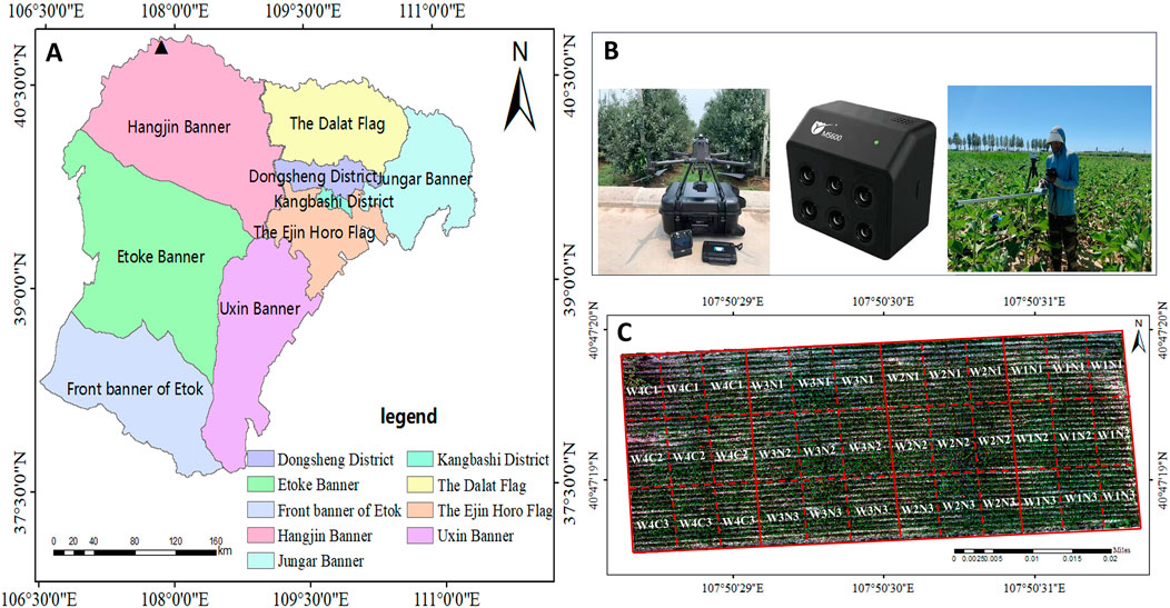
Figure 1. Location of the study area and test layout. (A) Ordos City, Inner Mongolia. (B) Field sampling photographs. (C) Layout of field trial plots.

The local maize variety “Ningyu 688″was tested. The experimental field was subjected to rotary tillage and leveling before sowing. In 2023, there were nine treatments in the experiment and each treatment was repeated three times. There were 27 plots, each with an area of 10 m × 4 m. The plots were arranged randomly. Maize planting in the experimental area was consistent with that in the local area, and film-mulched planting was adopted, with one film and two rows, film width of 60 cm, row spacing (wide spacing of 1 m, narrow spacing of 35 cm), and plant spacing of 23 cm. The planting density was 61,100 plants per hectare and the plants were sown on May 29th. This experiment used two variables, irrigation and fertilization, to form a comparative experiment. Three irrigation quotas were set: 50%, 75%, and 100% of the local irrigation volume (W1:150 m³/hm², W2:225 m³/hm², W3:300 m³/hm², respectively), irrigate eight times during the growth period, with drip irrigation as the irrigation method, and measure the irrigation water with a water meter. The three nitrogen application rates were set as N1:140 kg/hm², N2:210 kg/hm², N3:280 kg/hm², urea. They were applied at a ratio of 2:3:3:2 during the jointing, large trumpet mouth, stamening, and grain-filling stages without applying base fertilizer.

Based on the 2023 test, the 2024 test included three new treatments and set an irrigation quota (W4:225 m³/hm²). The three nitrogen application rates were C1:140 kg/hm², C2:210 kg/hm², and C3:280 kg/hm² (of which 30% was used as the base fertilizer and 70% as the top dressing); the remaining conditions were the same as those in the 2023 experiment. The specific irrigation and fertilization systems are listed in Table 1.

Table 1

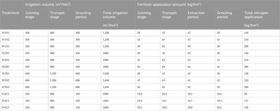
Table 1. Maize irrigation system.

2.2 Acquisition and processing of spectral images

2.2.1 Band introduction, image stitching, and other processing

ADJI M300RTK was used as the drone. The drone has a long flight time (55 min). The fuselage was also equipped with binocular vision and infrared sensors for omnidirectional perception up and down 30 m, and forward, backward, left, and right 40 m. It has a six-way obstacle avoidance function and features precise positioning and flexible flight. The UAV is equipped with Zenthink H20T and MS600 pro cameras, which include six multispectral bands, namely, blue (B, 450 ± 35 nm), green (G, 555 ± 25 nm), red (B, 660 ± 20 nm), red edge 1 (RE1, 720 ± 10 nm), and red edge 2 (RE2, 750 ± 15 nm), and near-infrared (NIR, 840 ± 35 nm). The Zenthink H20T comes standard with a 23x hybrid optical zoom system, 20-megapixel zoom camera, 12-megapixel wide-angle camera, and 1200-m laser rangefinder.

Spectral collection was mainly concentrated from June to September 2024 and was conducted at the jointing, large trumpet, tasking, filling, and maturity stages of maize. The flight time ranged from 10 a.m. to 12 p.m. The flight conditions were clear and cloudless, with open terrain and no obstructions. The flight parameters were set as follows: flight altitude of 20 m, take-off speed of 10 m/s, route speed of 1.2 m/s, overlap rate of both sidewalks and heading of 80%, and equal photo intervals. Before flight, black and white target cloths were arranged for the radiometric calibration of the multispectral images. The camera lens captured pictures directly above the crops during the flight. The flight parameters at each growth stage remained constant and were set prior to the first flight.

Drone images captured by cameras cannot be directly applied to the acquisition of remote sensing image data. It is necessary to use software pix4Dmapper to stitch the drone images. First, create a new project, import spectral photos, select AgMultispectral as the processing option template, and under the processing option DSM, under the Raster Digital Surface Model module in Orthophoto and Index, select GeoTiff and Synthetic tiles, then select GeoTiff and synthetic tiles in orthophoto images and start processing. Digital cameras can obtain characteristic maps of the B, G, and R indices, whereas multispectral cameras can produce reflectance maps of the red (red), green (green), blue (blue), rednir (near-infrared), and redage (red edge) bands. ENVI software was used for radiometric correction, band fusion, and setting the central wavelengths of each band to synthesize true-color image data. Finally, the reflectance values at each measurement site were extracted and used to calculate the vegetation index (VI).

2.3 Acquisition of ground measured data

UAV multispectral remote sensing data collection was conducted simultaneously with ground data collection, including crop height (CH) and LAI. CH and LAI measurements were used to establish and verify the estimation model. While collecting the data, the locations of the sampling points were recorded using a handheld GPS.

To measure the CH at each maize growth stage, three maize plants with uniform growth were selected from each plot. Plant height was measured and recorded using a tape measure. When measuring the LAI, at each maize growth stage, the LAI of each plot was measured using a Sunscan canopy meter. Six datasets were uniformly collected from each plot, and seventy-two were measured at the jointing, tasking, and filling stages of maize. The uniform distribution of data in each group was conducive for capturing spatial changes in vegetation and enhancing the representativeness and reliability of the data.

Determination of nitrogen content in plants: Place the plants at 105 °C for 30 min of blanching, then dry them at 75 °C until a constant weight is achieved, followed by crushing and sieving. After digestion with H2SO4-H2O2, the nitrogen content in various parts of the maize plant was determined using the Kjeldahl method. Seventy-two datasets were measured at each maize stage, and the average value was calculated as the final nitrogen content of each plot.

2.4 Extraction of canopy spectral information

2.4.1 Spectral information

Based on the literature, the reflectance of six spectral bands (B, G, R, RE1, RE2, and NIR are the blue light, green light, red light, red edge 1, red edge 2, and near-infrared bands, respectively) was utilized in this study. Based on these initial reflectance values, a set of VIs with 18 spectral variables was constructed for analysis. The spectral responses of maize LAI under different water and nitrogen treatments are shown in Table 2.

Table 2

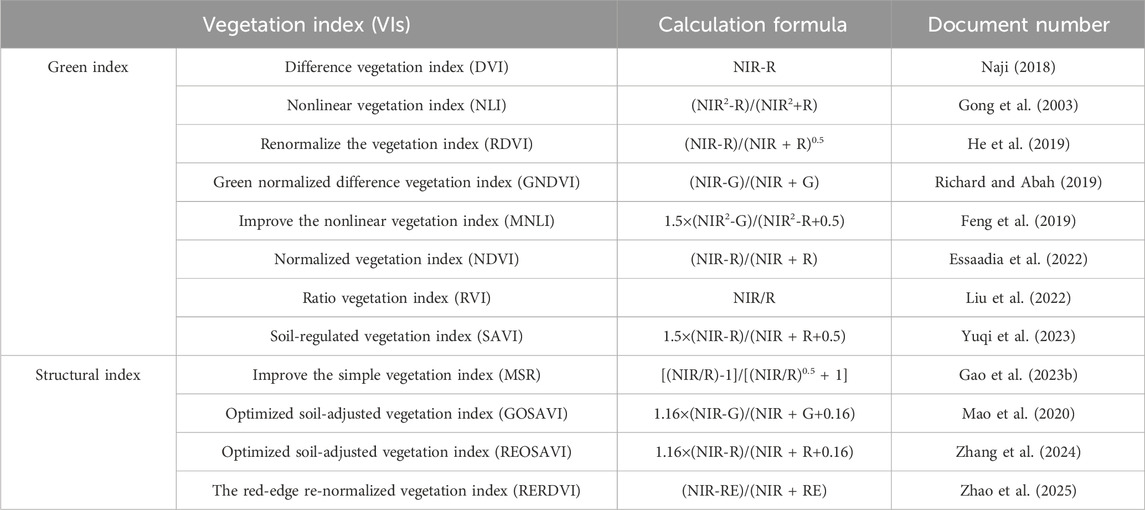
Table 2. Calculation of spectral parameters.

2.4.2 Texture information

In this study, ENVI5.6 software was used to extract image TFs based on second-order probabilistic statistical filtering. Eight TFs were obtained by extracting each band: mean (MEA), variance (AR), synergy (HOM), contrast (CON), dissimilarity (DIS), information entropy (ENT), second moment (SEM), and correlation (COR). During the texture analysis, the window size was selected as 7 × 7, and the default offsets X and Y of the spatial correlation matrix were 1. Through this method, the TFs of different bands can be effectively extracted from multispectral images, and these features can help us better understand the surface characteristics of ground objects. The second-order probabilistic statistical filtering method can describe the TFs of the surface of ground objects more accurately, which is helpful for applications such as ground object classification, change detection, and target recognition.

Similar to the calculation of the VI, the UAV multispectral system consisted of six bands with eight types of TFs in each band. Forty-8 TFs were obtained, and the TI was calculated by combining two different features, denoted as TIs. The texture metrics used in this study were the Normalized TI (NDTI), Differential TI (DTI), and Ratio TI (RTI). The calculation formula is shown in Equations 1–3, and are denoted as TIS.

$DTI=T_1-T_2(1)$

$\mathrm{N}DTI=\frac{T_1-T_2}{T_1+T_2}(2)$

$\mathrm{R}TI=\frac{T_1}{T_2}(3)$

T1 and T2 are the texture values of certain frequency bands screened based on TFs. The TFs used in this study are listed in Table 3.

Table 3

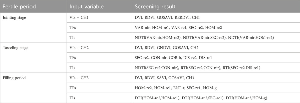
Table 3. Filter the input of the correlation threshold variable.

2.4.3 Structural information

In the bare soil, jointing, tasking, and filling stages of the study area, a DSM was generated using UAV multispectral images to extract the CH values of maize plant height at different periods. The DSM marker produced at the bare soil stage was DSM0, and the DSM markers extracted at each stage of crop growth were DSM (1,2,3). The CH was obtained by calculating the differences between DSM and DSM0 in each period, and the calculation formula is shown in Equation 4. At each growth stage of maize, the fitting accuracy R² between the predicted crop plant height from UAV images and the measured crop plant height was >0.8, showing a high degree of fitting. The height status of maize plants at different periods can be accurately predicted using UAV remote sensing, as shown in Figure 2.

${CH}_{\left(A,B,C\right)}={DSM}_{\left(A,B,C\right)}-{DSM}_0(4)$

Figure 2

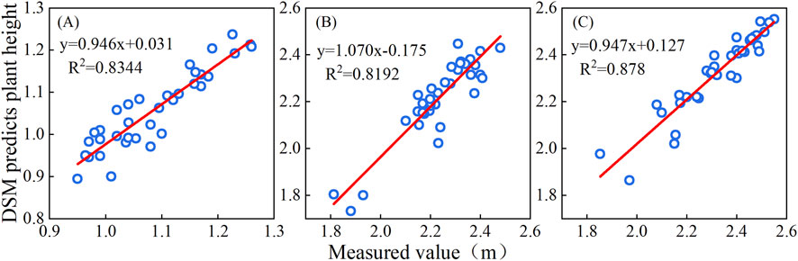
Figure 2. Relationship between the measured plant height calculated using remote sensing at different growth stages and the actual measured plant height. (A) Jointing stage. (B) Tasseling stage. (C) Grouting period.

2.5 Data analysis methods

The multispectral reflectance data of summer maize at the jointing, tasking, and filling stages were collected and combined with maize LAI data measured synchronously on the ground to form a sample dataset. Maize LAI was measured six times in each community using a Sunscan canopy meter. The averages of the measured values at each position were calculated, and 72 datasets were obtained. A model was constructed using the selected VI, CH, texture characteristics, TI, and LAI, including the modeling (2/3) and verification (1/3) sets. Comprehensively considering the significance levels of the sample data and LAI, the independent variables were screened to establish a machine learning model, namely, ridge regression (RR), and ensemble learning models, namely, random forest (RF) and convolutional neural network (CNN), thereby achieving high-precision estimation of maize LAI in various periods.

The Hill regression (RR) model provides an effective method for improving the generalization ability of linear regression models by balancing the relationship between the fitting data, controlling the complexity of the model, and adding a regularization term to the model to avoid overfitting and enhance its predictive ability. The RF model is an ensemble learning method. RF enhances prediction and model performance by combining multiple decision trees. CNN can perform unsupervised feature learning and automatically acquire features. Its architecture includes convolution, pooling, batch normalization, fully connected, discarded, and regression layers. The convolution kernel is set to half the number of input variables. The ReLU activation function was used to accelerate convergence. A dropout rate of 20% was set during training to prevent overfitting. The SGDM algorithm was used to optimize the weights. The initial learning rate was 0.01. Various machine, deep learning, and LAI inversion models were established using multiple learning packages, such as sklearn in PyCharm, and model fitting graphs were drawn using Origin 2021.

2.6 Model evaluation indicators

$R^2=\frac{{\displaystyle {\sum }_{i=1}^n}{\left(X_i-\overline{X}\right)}^2{\left(Y_i-\overline{Y}\right)}^2}{{\displaystyle {\sum }_{i=1}^n}{\left(X_i-\overline{X}\right)}^2{\displaystyle {\sum }_{i=1}^n}{\left(Y_i-\overline{Y}\right)}^2}(5)$

$RMSE=\sqrt{\frac{{\displaystyle {\sum }_{i=1}^n}{\left(Y_i-\overline{Y}\right)}^2}{n}}(6)$

$RPD=\frac{SD\left(xi\right)}{RMSE}(7)$

where $X_i$, $\overline{X}$, $Y_i$, and $\overline{Y}$ represent the measured, measured average, estimated, and estimated average values, respectively, and n represents the number of samples in the model. The model accuracy was evaluated using the coefficient of determination R², root mean square error (RMSE), and the ratio of performance to standard deviation (RPD). When the coefficient of determination R² was larger, the prediction effect of the model was better, the RMSE was smaller, and the model was more accurate. It is generally believed that RPD<1.4 indicates that the model is unreliable, 1.4<RPD<2.0 indicates that the model has moderate reliability, and if RPD>2.0, the model has higher reliability. SD is the standard deviation of the measured values of the sample. The calculation formula is shown in Equations 5–7.

2.7 Construction of the critical nitrogen concentration model

2.7.1 Model construction

Critical nitrogen concentration refers to the critical value of the nitrogen concentration at which the LAI of the plant is the largest at each stage of crop growth. When the nitrogen concentration in a plant is below the critical nitrogen concentration, growth is restricted. When the nitrogen concentration of the plant exceeded the critical nitrogen concentration, nitrogen had no obvious effect on the LAI of the crop. Instead, the excess activated nitrogen in the soil is lost, which causes environmental pollution. According to the critical nitrogen concentration dilution model theory proposed by previous researchers, the construction of a curve model was divided into the following steps:

1. The predicted LAI values of different fertilization treatments were obtained using the model, the corresponding plant nitrogen concentrations were determined, and whether crop growth was restricted by nitrogen was determined through analysis of variance.

2. Function fitting was performed on the predicted values of the nitrogen-restricted LAI and the corresponding nitrogen concentrations.

3. The maximum predicted LAI value of the test material under unrestricted growth was obtained.

4. The theoretical critical nitrogen concentration was the maximum LAI on each sampling date on the corresponding vertical coordinates of the function.

According to the definition of the critical nitrogen concentration dilution curve, the calculation formula is shown in Equation 8:

$N_a=a\times LA{I}^{-b}(8)$

In this study, to establish the critical nitrogen concentration curves under different irrigation conditions and improve the accuracy of the model, irrigation and density factors were added. The calculation formula is shown in Equation 9:

$N_a=a\times LA{I}^{-b}\times \left(1+c\times K\right)-d\times D(9)$

where a, b, c, and d are coefficients; K is the irrigation factor (normalizing the different irrigation treatments in this study); and D is the density factor.

2.7.2 Test of the critical nitrogen concentration dilution model

The critical nitrogen concentration dilution model was verified using the RMSE and standard mean square error (n-RMSE). Its reliability and degree of fit were determined using a 1:1 histogram of the measured and simulated values. The smaller the RMSE value, the smaller the deviation between the simulated and measured values. n-RMSEs of <10%, 10% and 20%, 20% and 30%, and >30% indicate extremely good, relatively good, average, and poor simulation performances, respectively. The calculation formula is shown in Equations 10, 11

$\mathrm{R}MSE=\sqrt{\frac{{\displaystyle {\sum }_{i=1}^n}\left(B_i-F_i\right)}{n}}(10)$

$\mathrm{n}-RMSE=\frac{RMSE}{mean\left(B_i\right)}(11)$

where Bi represents the measured value, Fi is the simulated value, and n is the sample size.

2.7.3 Nitrogen nutrition index (NNI) model

The NNI refers to the ratio of the actual nitrogen concentration of crops to the critical nitrogen concentration, which can be used to reflect the nitrogen nutrition situation of drip-irrigated maize more accurately. Based on the critical nitrogen concentration dilution model, the concept of the NNI was proposed, the calculation formula is shown in Equation 12:

$NNI=\frac{N_i}{N_c}(12)$

where Ni represents the measured nitrogen concentration (%) of the drip-irrigated maize and Nc represents the simulated value (%). When NNI = 1, the nitrogen nutritional level in the plant body was optimal. An NNI > 1 indicates an excess of nitrogen nutrition and an NNI < 1 indicates insufficient nitrogen nutrition.

2.8 Workflow of this research

Figure 3 presents the workflow of this study. First, a multispectral sensor installed on an UAV was used to obtain maize canopy images in the study area. Farmland image maps of maize at various growth stages were obtained using methods such as image stitching, radiation correction, and band fusion. Based on these images, the VIs, TFs, TIs, and CH were extracted. Second, correlation analysis was conducted to select optimal remote sensing indicators and their combinations. The above-mentioned combined indicators were used as independent variables, and the measured LAI values were used as dependent variables. Three models were established: CNN, RF, and RR. Two-thirds were used for the modeling set and one-third for the validation set. The accuracy of the model was evaluated using the coefficient of determination (R²), RMSE, and RPD. Subsequently, the LAI-predicted data and measured nitrogen content of the leaves were obtained using the optimal model. A critical nitrogen concentration dilution curve model was constructed, the critical nitrogen concentration curve was improved, and the curve was verified using 2023 data. A NNI model was constructed to clarify the fertilizer dosage for each treatment at different growth stages, and to formulate a fertilization system that provides a reference for precise fertilization in agriculture.

Figure 3

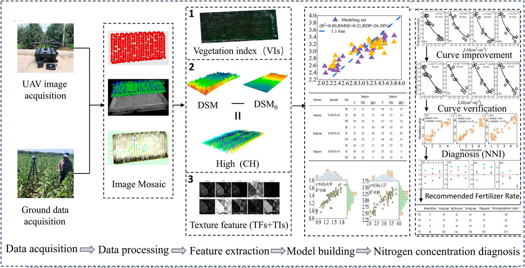
Figure 3. Flowchart of this study.

3 Results and analysis

3.1 Changes in maize growth parameters

The LAI and leaf nitrogen content of maize at different growth stages are shown in Figure 4. As the growth period progressed, the LAI of different treatments gradually increased, whereas the nitrogen content of the leaves showed a gradually decreasing trend. During the jointing stage, the LAI of maize was approximately 1.5, and the LAI of the treatment with base fertilizer was relatively larger than that of the treatment without base fertilizer. Under the 12 different treatment conditions, the nitrogen content of the leaves did not vary significantly and was generally close to 4% (Figure 4A). During the tasking stage, the LAI of maize under different treatments showed significant changes. The LAI under the low fertilizer treatment was significantly smaller than that of the high and medium fertilizer treatments, indicating that fertilization significantly impacted the growth of maize leaves. The nitrogen content of the maize leaves during this period was close to 3% (Figure 4B). During the filling period, the LAI of maize under different treatments varied slightly. The low-water irrigation condition was smaller than that of the other irrigation treatments, and the overall LAI reached 4.5 (Figure 4C). The nitrogen content in the maize leaves during this period was approximately 2%. The LAI of maize increased rapidly from the jointing stage to the tasseling stage but increased relatively slowly from the tasseling stage to the filling stage. The nitrogen content of leaves gradually decreased and reached a minimum during the filling period. The growth of the maize LAI was inversely correlated to the nitrogen content of the leaves.

Figure 4

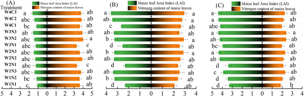
Figure 4. Maize LAI and leaf nitrogen content under different treatment conditions. (A) Jointing stage. (B) Tasseling stage. (C) Grouting period.

3.2 Correlation analysis of maize LAI and spectral variables

Based on the multispectral images, the VI was calculated using the six extracted single-band reflectance rates: B, G, R, RE1, RE2, and NIR. The maize CH retrieved by remote sensing and the measured LAI values of the corresponding plots were added to construct the sample dataset. A correlation analysis was conducted between the measured LAI values and spectral variables during the jointing, tasking, and filling stages. Seventy-two samples were collected during each growth period. During the maize germination stage, the NIR, Ratio VI (RVI), and Improved Simple VI (MSR) had a relatively weak correlation with LAI, and the Nonlinear VI (NLI), Green Normalized Difference VI (GNDVI), Improved NLI (MNLI), Soil-adjusted VI (SAVI), and Red-edge Optimized SAVI (REOSAVI) showed negative correlations. Among them, the Green Optimized SAVI (GOSAVI) had the most obvious correlation with LAI (0.57), whereas CH1 also had a relatively high correlation with LAI (0.55). The Difference VI (DVI), Re-normalized VI (RDVI), GOSAVI, Red-edge Re-normalized (RERDVI), and CH1 were selected as the VIs for the input model at the jointing stage (Figure 5A). During the maize tasseling period, VIs such as the NIR, NLI, MNLI, MSR, and REOSAVI showed a relatively small correlation with LAI, whereas RVI showed a negative correlation. Among them, GOSAVI had the most obvious correlation with LAI (0.56), whereas CH2 had a relatively high correlation (0.41). The DVI, RDVI, GNDVI, GOSAVI, and CH2 were selected as the VIs for the input model during the tasseling period (Figure 5B). Using the same analysis method, DVI, RDVI, SAVI, GOSAVI, and CH3 were selected as the VIs for the input model during the filling period (Figure 5C).

Figure 5

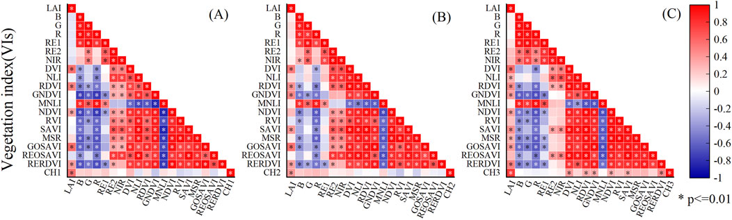
Figure 5. Correlation between VI and LAI in different periods. (A–C) represent the jointing, tasseling, and grouting stages, respectively. Abbreviations of the specific VIs are shown in Table 2.

3.3 Correlation analysis of maize LAI with texture characteristics and index

Correlation analysis was conducted using the measured LAI of maize at various stages and the TFs constructed using the six single bands (B, G, R, RE1, RE2, and NIR) of the UAV multispectral images. At each growth stage of maize, 48 groups of TFs were observed. Five TFs with the highest correlation with the LAI were selected to construct the model. During the jointing stage, VAR-nir, HOM-re1, VAR-re1, SEC-re2, and HOM-re2 were selected as the TFs of the model input, with correlations of 0.42, 0.41, 0.38, 0.36, and 0.35, respectively (Figure 6A). During the maize tasseling period, using the same method, SEC-re2, CON-nir, COR-b, DIS-re2, and DIS-re1 were selected as the TFs of the model input, with correlations of 0.54, 0.48, 0.38, 0.38, and 0.34, respectively (Figure 6B). During the growth and filling stages, HOM-re2, HOM-re1, ENT-r, SEC-re1, and HOM-g were selected as the TF inputs to the model, with correlations of 0.5, 0.46, 0.46, 0.42, and 0.4, respectively (Figure 6C).

Figure 6

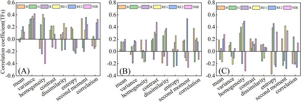
Figure 6. Correlation between texture characteristics and LAI in different periods. (A) Jointingstage. (B) Tasselingstage. (C) Groutingperiod.

TFs with high correlations in each period were selected to construct a NDTI, DTI, and RTI. Three texture indices with high correlations with maize LAI were selected as independent variables for model construction (Figure 7). At the jointing stage (Figure 7A), NDTI(VAR-nir,HOM-re2), NDTI(VAR-nir,SEC-re2), and NDTI(VAR-nir,HOM-re1) were selected for model construction. During the tassel extraction period (Figure 7B), NDTI(SEC-re2,CON-nir), RTI(SEC-re2,CON-nir), and RTI(SEC-re2,DIS-re1) were selected. During the grouting period (Figure 7C), DTI(HOM-re2,HOM-re1), DTI(HOM-re2,SEC-re1), and DTI(HOM-re2,HOM-g) were selected.

Figure 7

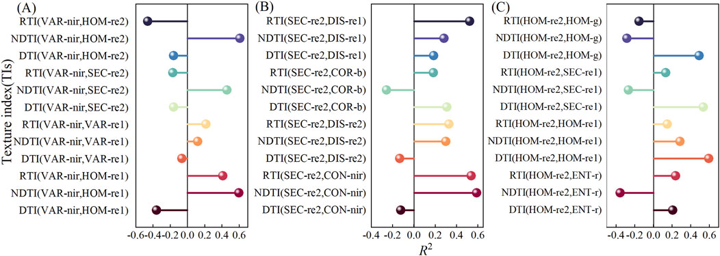
Figure 7. Correlation between TI and LAI in different periods. (A) Jointingstage. (B) Tasselingstage. (C) Groutingperiod.

3.4 LAI estimation based on data fusion

The accuracy of multi-feature fusion was significantly improved compared to the univariate feature model. Multi-feature fusion can better describe the changes in crop growth patterns. Therefore, in this study, the process of constructing the model using univariate features was reduced, and the four features were directly fused for model construction.

From 2023 to 2024, multispectral image data were obtained during the jointing, tasseling, and filling stages of maize. Four VIs and predicted plant height (CH) values for crops, 5 TFs, and three texture indices, totaling thirteen groups of characteristic variables, were used to construct the model. The selection conditions are listed in Table 3. The 13 selected eigenvalues were taken as independent variables, and the LAI values for each period were taken as dependent variables. The independent variables were divided into a training set (accounting for 2/3 of the total sample) and a validation set (accounting for 1/3 of the total sample) using the random sampling method to ensure the wide applicability of the constructed model. The training sets were then input into the RR, RF, and CNN models. The models constructed for different periods are shown in Figure 8. In comparison, the RF model exhibited the highest estimation accuracy. The R² values of the modeling sets at the different growth stages were 0.84, 0.80, and 0.87, which were >25% higher than those of the RR and CNN models. The RMSE values were 0.11, 0.21, and 0.15, which were >20% lower than those of the other models, indicating that the RDP parameters were relatively reliable. The R² values of the RF model validation set were 0.61, 0.63, and 0.73, which increased by >22% compared with those of the RR and CNN models, and the RMSE decreased by >15%. Compared with the RR and CNN models, the RF model showed a better effect in inverting the maize LAI. This is possibly because, from the perspective of the model principle, RR is an improved form of linear regression. Although the regularization term is robust, it limits the complexity and makes it difficult to fit the complex nonlinear relationships of the maize image data. The accuracy of the CNN model was lower than that of the ensemble learning RF. One possible reason is that a CNN requires many diverse samples to fully learn the inherent laws and feature patterns of the data. However, in this study, there were only 72 samples in each period, making it difficult to support the CNN model. RF can effectively handle high-dimensional data. Although the sample size was small, the multi-dimensional data information contained in the samples, such as multispectral images, VI, and TFs, RF can fully mine valuable information in the data from different perspectives through multiple trees and has a good predictive ability for the LAI of maize. Therefore, in this study, RF based on feature fusion demonstrated high model accuracy and could effectively invert the dynamic changes in maize LAI at different growth stages.

Figure 8

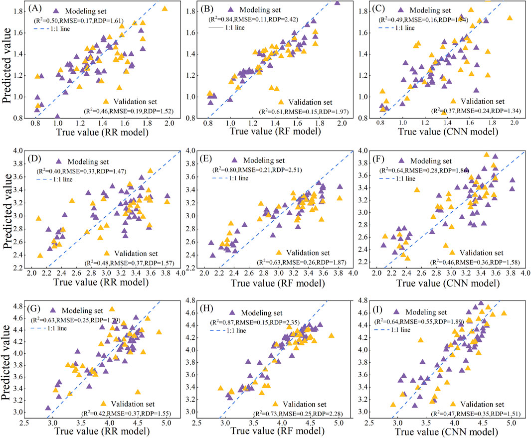
Figure 8. Comparison chart of various learning models at different growth stages. (A–C) represent a comparison of the modeling accuracy of the different models during the jointing stage. (D–F) represent a comparison of the modeling accuracy of the different models during the tasseling period. (G–I), represent a comparison of the modeling accuracy of the different models during the grouting period. RR is the ridge regression model, RF is the random forest model, and CNN is the Convolutional Neural Network model. R² is the coefficient of determination, RMSE is the root mean square error, and RDP is the residual prediction deviation.

The predicted LAI values for maize at each growth stage were obtained using the RF and fitted to the measured values. The model showed high fitting accuracy at each maize growth stage. The results are presented in Figure 9. The fitting accuracies at the jointing, tasseling, and filling stages were 0.80, 0.82, and 0.83, respectively. Moreover, the LAI generally remained between 0.9 and 1.8, 2 and 4, and 3 and 4.8 during the jointing, emasculation, and filling stages, respectively. The variation patterns of the estimated and measured LAI values at the three growth stages were consistent. RF shows a good estimation ability. Some researchers have used different learning models to estimate the maize LAI and found that RF showed a better effect. This result verifies the effectiveness of the multi-source information fusion strategy and provides a reference for other researchers when inverting the maize LAI.

Figure 9

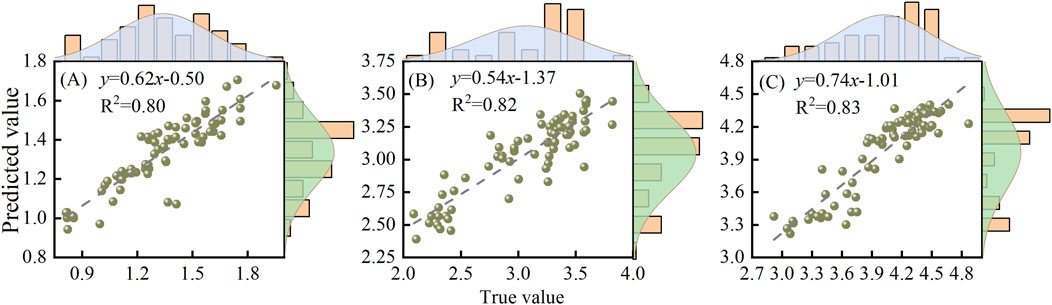
Figure 9. Comparison chart of model-predicted LAI and measured values. (A) Jointing stage. (B) Tasseling stage. (C) Grouting period.

3.5 Construction and improvement of the critical nitrogen concentration dilution curve model

The leaf area indices of plants at different nitrogen application levels were obtained according to the definition of the critical nitrogen concentration dilution curve, and the corresponding nitrogen concentrations of the plants were determined. Analysis of variance was used to determine whether crop growth was limited by nitrogen. Functional fitting was performed between the leaf area under nitrogen limitation and the corresponding nitrogen concentration. The maximum LAI of the experimental material with unrestricted growth was substituted into the equation for the calculation. The corresponding vertical coordinates represent the critical nitrogen concentrations. In this study, a variance analysis was conducted for each treatment. Under the irrigation condition of W1, treatments N1 and N2 were the nitrogen-restricted groups and N3 was the non-nitrogen-restricted group. Under the remaining irrigation treatment conditions, N1 was the nitrogen-restricted group, and N2 and N3 were the non-nitrogen-restricted groups. There were three sampling values for each treatment. The dilution curves of the critical nitrogen concentration in leaves based on summer maize LAI under different moisture treatments are shown in Figure 10.

Figure 10

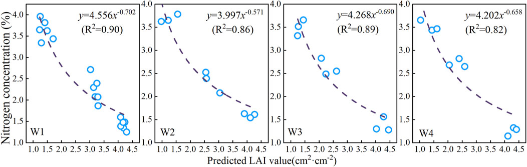
Figure 10. The critical nitrogen dilution curve based on the LAI of summer maize. W1, W2, W3, and W4 represent different irrigation treatments. For further details, see Table 1.

The nitrogen concentration of each irrigation treatment showed a downward trend with an increase of the predicted LAI value, and its change process was fitted by the power function equation. In the critical nitrogen concentration dilution curve model, the power function fitting parameters a for the W1, W2, W3, and W4 irrigation treatments were 4.556, 3.997, 4.268, and 4.202, and those for parameters b were −0.702, −0.571, −0.690, and −0.658, respectively. Because the classification of nitrogen restriction groups in the W1 treatment was different from that in other irrigation treatments, excluding the W1 treatment, parameter a of the other treatments increased with an increase in irrigation water volume, and parameter b decreased with an increase in irrigation water volume. This meets the general characteristics of constructing the critical nitrogen concentration curve, which had a relatively high accuracy. The R² values under the W1, W2, W3, and W4 irrigation conditions were 0.90, 0.86, 0.89, and 0.82, respectively.

Based on the above critical nitrogen concentration curve, the original form of the critical nitrogen concentration curve is Na = a × LAI^-b. This curve was improved, and the improved form of the curve is Na = a × LAI^-b × (1 + c × K)-d × D, where a, b, c, and d are variable coefficients. Because critical nitrogen concentration dilution curves were established in this study under different irrigation conditions, the irrigation factor K was introduced to normalize the irrigation volume of the different irrigation treatments. After normalization, K (w1) = 0, K (w2) = 0.5, K (w3) = 1, and K (w4) = 0.5. The density factor D was 6 plants/m³. Critical nitrogen concentration curves improved under different irrigation conditions (Figure 11). Under the irrigation condition of W1, the critical nitrogen concentration curve R² after improvement showed no significant change compared to that before improvement. Therefore, the critical nitrogen concentration curve for W1 irrigation did not improve. Under the W2 irrigation condition, the R² of the improved critical nitrogen concentration curve was 0.89, which was 3.37% higher than that before the improvement. Under the W3 irrigation condition, R² was 0.92, which was 3.26% higher than that before the improvement. Under the W4 irrigation condition, R² was 0.89, which was 7.87% higher than that before the improvement. Under different irrigation conditions, the R² of the critical nitrogen concentration curve after improvement increased compared to that before improvement. Therefore, these results provide a theoretical basis and methodological reference for establishing dilution curves for critical nitrogen concentration in crops under different irrigation conditions.

Figure 11

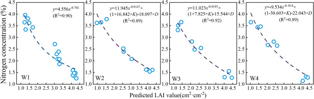
Figure 11. Improvement of the critical nitrogen dilution curve based on the LAI of summer maize.

3.6 Verification of the critical nitrogen concentration dilution curve model

This study used data from 2024 for model construction and independent data from 2023 for verification. Because no W4 irrigation treatment was set up in 2023, only three types of water treatments were verified. For the LAI of drip-irrigated maize under the three moisture conditions on each sampling day in 2023, three sets of duplicate data were taken and substituted into the model to obtain the simulated values. Figure 12 shows a histogram of the 1:1 relationship between the measured and simulated values under different moisture conditions. Under the three moisture conditions, the RMSE values were 0.38, 0.6, and 0.6, and the n-RMSE values were 13.9%, 18.7%, and 17.5%, respectively. By integrating the RMSE and n-RMSE values, the simulation effect of the model was shown to be good, and the model accuracy was high. This method can be applied to the nitrogen nutrition diagnosis of drip-irrigated maize under different moisture conditions.

Figure 12

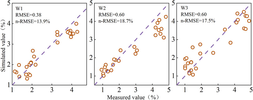
Figure 12. Verification graph of the critical nitrogen concentration curve.

3.7 Construction of NNI model and recommendation of fertilizer application amount

Figure 13 shows that during the maize growth process, the NNI in the upper ground is not uniform and fluctuates dynamically. The variation trend of the NNI under different water treatment conditions at different growth stages had a significant relationship with the amount of fertilization at the growth stage. In this experiment, the ratio of the top dressing amount at each growth stage was 2:3:2 for the jointing, tasseling, and filling stages. Under the W1 irrigation condition, during the jointing (V6) and the grain-filling (V8) stages, the NNI at the N3 topdressing amount was close to 1, whereas under the N2 and N1 conditions, the NNI values were all below 1. Water shortage may lead to low fertilizer utilization efficiency, resulting in fertilizer deficiency in the N2 and N1 treatments. Under the conditions of relatively sufficient irrigation in W2 and W3, the NNI in the N3 treatment was >1, the NNI in the N2 treatment remained approximately 1, and the NNI in the N1 treatment was <1. Under the condition that irrigation in W4 was relatively sufficient, base fertilizer was applied before sowing in the W4 treatment. Therefore, during the jointing stage (V6), the NNI of the N3 treatment was >1, whereas that of the N2 treatment was approximately 1. As the growth period progressed, the amount of top dressing used in the W4 treatment was relatively small. Therefore, during the emasculation and filling stages, the NNI under the N3 treatment was close to 1, whereas those under the N2 and N1 treatments were <1.

Figure 13

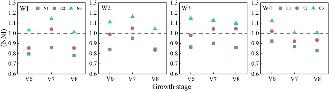
Figure 13. Dynamic changes in NNI in summer maize leaves under different water and nitrogen treatments. V6: Jointing stage V7: Tasseling stage V8: Grouting period.

When the NNI is between 0.9 and 1.1, nitrogen is considered to be in an appropriate condition. Based on the comparison of the fertilization levels of each irrigation treatment with an NNI close to 1 (Figure 11), the fertilization system for the growth period of this experiment was roughly formulated Table 4. According to the critical nitrogen concentration dilution curve, the fertilizer application amounts for each irrigation treatment were optimized as follows: Under the condition of no base fertilizer treatment and horizontal irrigation of W1, the total nitrogen application amount was 238 kg/hm²; under the condition of horizontal irrigation of W2, the total nitrogen application amount was 224 kg/hm²; and under the condition of horizontal irrigation of W3, the total nitrogen application amount was 210 kg/hm². When the irrigation condition was W4, the base fertilizer was applied at 84 kg/hm², top dressing amount at 171.5 kg/hm², and total nitrogen application amount at 255.5 kg/hm². After comparing the growth conditions and yield factors of maize under different treatments, the mixed application mode of base fertilizer and top dressing was better for the overall growth of maize. Therefore, in the maize planting process in this area, W4 irrigation and the fertilization mode of the base fertilizer and top dressing are the most recommended, with a total nitrogen application rate of 255.5 kg/hm². Among them, 84 kg/hm² was applied as base fertilizer, 29.4 kg/hm² during the jointing stage, 44.1 kg/hm² during the large trumpet mouth stage, 58.8 kg/hm² during the emasculation stage, and 39.2 kg/hm² during the grain filling stage.

Table 4

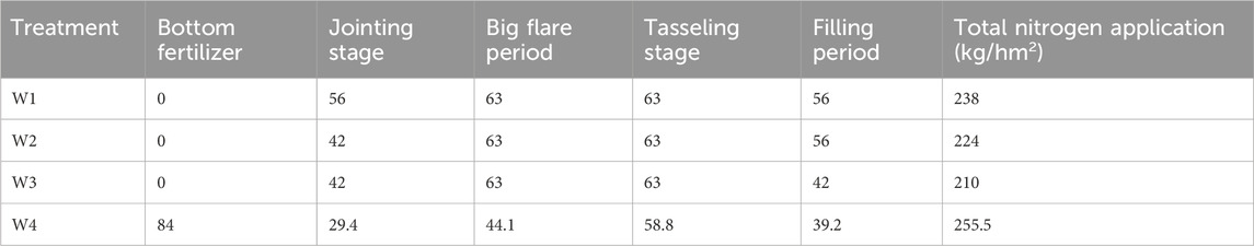
Table 4. Recommended fertilizer application amounts.

4 Discussion

4.1 Changes in LAI and leaf nitrogen content of maize at different periods

The LAI and leaf nitrogen content of maize are important indicators of plant growth and play key roles in photosynthesis, nutrient absorption, and plant growth and development (Chi et al., 2023). LAI represents the growth status of plants and determines the photosynthetic efficiency and yield of maize, whereas the nitrogen content in leaves directly affects the growth and overall nutritional status of plants. In this study, the effects of water-nitrogen coupling on the LAI value and nitrogen content of maize leaves were studied through a field experiment involving drip irrigation under film. Research has found that, with the advancement of the growth period, the LAI value of maize generally shows a trend of first increasing and then decreasing. In the early stages of grain filling, the LAI of maize reached its maximum value, and at this time, maize growth stopped. However, in the later stage, with the maturity of the maize, the LAI value decreased significantly. The LAI value of maize in each treatment during the jointing stage was generally maintained at approximately 1.5, and was maintained between 3 and 4 during the tasseling stage. The grouting period was approximately 4.5. The overall trend of nitrogen content in the maize leaves was inversely proportional to the LAI. As the growth period progressed, the nitrogen content in the maize leaves gradually decreased. The nitrogen contents in the maize leaves under each treatment during the jointing, tasseling, and filling stages were generally maintained at approximately 4%, 2%, and <2%, respectively.

4.2 Multi-feature fusion methods and optimal model selection

In the current field of crop physiological parameter inversion research, model construction methods based on a single variable have gradually been replaced by multivariable fusion models, and the multivariable feature fusion approach has become mainstream (Su et al., 2024). Previous studies have found that multiple features mainly include VI, TFs, TI, predicted crop plant height, and coverage (Zhou et al., 2023). The main purpose of this study was to explore the potential of using different learning models to improve the accuracy of estimating the LAI of maize at various growth stages by combining VIs, CH, TFs, and TIs based on UAV multispectral images. This study revealed a robust correlation between the VI and the LAI of maize at different growth stages. During the maize jointing stage, the VIs with higher correlations were DVI, RDVI, GOSAVI, and RERDVI; those during the tasseling period were DVI, RDVI, GNDVI, and GOSAVI; and those during the grouting period were DVI, RDVI, SAVI, and GOSAVI. These indices sensitively capture the changes in vegetation structure and coverage rate, thereby indicating a significant positive correlation with LAI. Indicators such as DVI, RDVI, and GOSAVI were selected during the three growth stages of maize. These indices were corrected for atmospheric influence and soil background, effectively reducing the interference of vegetation reflectance and providing more accurate information about the maize LAI. Therefore, these indices are significantly correlated with LAI (Liu et al., 2023).

However, some researchers believe that the correlation between most TFs and LAI is relatively weak, and the extraction of TFs is often affected by factors such as the atmosphere, light, and soil background (Zou et al., 2024). Therefore, in this study, while selecting TFs with high correlation, a diverse and comprehensive TI was constructed by combining TFs with high correlation. TFs were combined to eliminate this influence. The NDTI, DTI, and RTI formed by the combination of each band were highly correlated with the LAI value. Moreover, the normalized, difference, and ratio texture indices improved the monitoring accuracy and anti-interference ability of the crops through standardization, difference amplification, and ratio operations. They are suitable for multiple growth stages and complex environments, and better reflect the canopy structure of maize (Fan et al., 2023).

Some researchers also believe that combining crop structure indices, such as CH, can significantly improve model accuracy. During the growth and development of maize, there was a positive correlation between CH and LAI. Adding plant height information can compensate for the deficiency of multispectral data in vertical structure characterization. Through the synergistic effect of three-dimensional morphological and spectral reflection characteristics, the inversion accuracy of LAI is improved, and the robustness of the model against differences in planting density and lodging stress is enhanced, making it suitable for dynamic monitoring of LAI throughout the growth period (Zhao et al., 2024). Therefore, in the process of inverting the maize LAI in this study, the structural information, CH, was added. Moreover, in this study, a high accuracy was achieved in extracting CHs using UAV images. The R² values of the measured and predicted values for each period were 0.8344, 0.8912, and 0.878. Meanwhile, some researchers believe that it is not particularly significant to first construct a model using a single feature variable and then use multiple feature variables to build a model and compare the accuracies among them because the model constructed using fused features must have higher accuracies. Therefore, in this study, the process of constructing a model using a single feature variable was not performed; the model was constructed directly using multiple features. This research found that at three different growth stages of maize, the RF model showed high accuracy. The R² values of the modeling sets for the jointing, tasseling, and grain-filling stages were 0.84, 0.80, and 0.87, with RMSE values of 0.11, 0.21, and 0.15, respectively. The R² values of the validation sets were 0.61, 0.63, and 0.73, and the RMSE values were 0.21, 0.26, and 0.25, respectively, and the RDP was in an ideal state. The R² values of the RF testing and validation sets were >25% higher than those of the RR and CNN, and the RMSE was 20% lower. Through multimodal data collaboration, nonlinear modeling, and a self-service sampling mechanism, the RF deeply explores the interaction of spectral–structural–texture features. The decision tree automatically learns the dynamic adjustment of the feature weights during the growth period, enabling the model to achieve high accuracy. The CNN and RR algorithms performed poorly. A possible reason for this is the insufficient number of training samples used. The limited scale of the dataset restricts the full advantage of the deep learning model, resulting in the failure of its nonlinear feature extraction ability to be effectively transformed into performance improvement. However, deep learning has significant advantages for processing large-scale data (Ahmed et al., 2023). Monitoring the growth status of crops using remote sensing will be a trend for future research. Satellite remote sensing images, with their wide coverage and multitemporal characteristics, can form a spatiotemporal complementarity with UAV data in terms of their spectral and texture information (Zhu et al., 2018). The feature fusion method can improve the accuracy of crop monitoring at a regional scale by integrating data sources from multiple platforms (Himeur et al., 2022).

4.3 Improvement of the critical nitrogen concentration dilution curve and optimization of nitrogen application rate

The critical nitrogen concentration dilution curve based on the dry matter of plants has been widely applied to crops such as maize, sunflower, rice, cotton, and chili peppers. Moreover, factors such as planted crops, planting regions, and water and fertilizer management affect the critical nitrogen concentration dilution curve (Liu et al., 2024). However, the construction of a critical nitrogen concentration curve based on the dry matter of plants is relatively cumbersome, and the dry matter collection process is time-consuming and laborious. The LAI can also be used to construct a critical nitrogen concentration curve. With the wide application of technologies such as LAI detectors and remote sensing in agriculture, constructing a curve using the LAI has become convenient (Liu et al., 2024). Therefore, in this study, the predicted values of maize LAI was obtained using the RF model. Combined with the nitrogen content of maize leaves, dilution curves of the critical nitrogen concentration under different water treatments were constructed. The accuracies of each irrigation treatment were as follows: R² = 0.90, R² = 0.86, R² = 0.89, and R² = 0.82 under W1, W2, W3, and W4, respectively. Moreover, as the maize growth period progressed, the LAI gradually increased, whereas the nitrogen content in the leaves gradually decreased. This is consistent with the rule of constructing curves using dry matter. Furthermore, based on the construction of critical nitrogen concentration curves for the different irrigation treatments in this study, the curve was improved. The form of the improved curve was Na = a × LAI^-b (1 + c × K)-d × D, where K was obtained by normalizing the irrigation volume of each irrigation treatment. After normalization, K (w1) = 0, K (w2) = 0.5, and K (w3) = 1. K (w4) = 0.5 D represents the planting density. For W1 irrigation, K was 0. The accuracy R² of the critical nitrogen concentration curve after improvement did not increase significantly compared to that before improvement. Considering the complexity of the curve form after improvement, the W1 irrigation treatment was not applied in this curve improvement. The accuracy of the model after other treatments improved to varying degrees compared with that before the improvement. Nitrogen deficiency was determined based on the NNI models for each treatment. When the NNI is between 0.9 and 1.1, nitrogen is considered to be in an appropriate condition. According to these conditions, in this experiment, the NNI model was used to determine the most suitable fertilizer application amount during the growth period. Combined with the growth status and yield requirements of maize during the growth period, the irrigation and fertilizer application amount is determined as follows. The most recommended irrigation method is W4, which involves a combination of base fertilizer and top dressing. Specifically, the base fertilizer should be applied at a rate of 84 kg/hm², 29.4 kg/hm² during the jointing stage, 44.1 kg/hm² during the large trumpet mouth stage, 58.8 kg/hm² during the emasculation stage, and 39.2 kg/hm² during the grain filling stage. The total nitrogen application rate was 255.5 kg/hm².

The advantage of this study is that when most researchers use UAV remote sensing to invert crop indicators, they only consider technical means, such as comparing multiple models and combining multiple methods, to improve the inversion accuracy of the models. These technical methods only remain at the theoretical and technical levels, fail to be effectively related to actual ground scenes, such as farmland, and lack practical application value. However, the present study did not address these limitations. After the inversion of the LAI, a critical nitrogen concentration curve was constructed and improved. The improved critical nitrogen concentration dilution curve precisely matched the requirements of different irrigation and planting densities, overcoming the limitations of the universality of traditional curves and contributing a new perspective to the construction of the critical nitrogen concentration curve.

5 Conclusion

This study utilized multispectral images from UAVs to extract spectral and texture features, while incorporating plant height information to estimate the LAI of maize. The effectiveness of different algorithms in predicting the LAI values of maize was evaluated through a comparative analysis. The estimated LAI values were used to construct a critical nitrogen concentration curve, which was then improved based on actual field conditions to formulate fertilization plans for each growth stage. The main conclusions are as follows.

1. The combination of TFs can significantly enhance the correlation between TFs and maize LAI. The CH value extracted from UAV images plays an important role in LAI estimation. Combining feature information can significantly improve the LAI estimation accuracy. Machine and deep learning algorithms have achieved satisfactory results in accurately estimating the maize LAI using UAV remote sensing data.

2. By integrating the irrigation and density factors, the critical nitrogen concentration curves under different irrigation treatments were improved. The improved R² values are 0.90, 0.89, 0.92, and 0.89 compared with the R² values before improvement (0.90, 0.86, 0.89, and 0.82, respectively), and the average improvement was 3.5%. After improvement, the curves eliminated the fitting deviations of the traditional model under high-density planting or water stress conditions, providing a basis for constructing critical nitrogen concentration curves under different irrigation treatments.

3. After comparing the NNI model and combining the growth and yield information of the crops during the reproductive period, a reasonable fertilization plan was formulated. The optimal mode for maize cultivation in this area was determined to be the split application of the base fertilizer and topdressing under W4 irrigation conditions. The specific plan is as follows: apply 84 kg/hm² of pure nitrogen as base fertilizer, followed by 29.4 kg/hm² during the jointing stage (accounting for 11.5% of the total), 44.1 kg/hm² during the large-flower stage (accounting for 17.2%), 58.8 kg/hm² during the tasseling stage (accounting for 23.0%), and 39.2 kg/hm² during the filling stage (accounting for 15.3%). The total amount of nitrogen applied throughout the growth period was 255.5 kg/hm². This plan provides a scientific basis for high-yield and high-efficiency maize cultivation on the southern bank of the Yellow River region by precisely regulating the nitrogen supply intensity during the growth period.

4. This study has some limitations in predicting the maize LAI using multiple features. The structural features in this study only describe the extraction of the CH. In subsequent studies, the three-dimensional structural features of the canopy, such as maize porosity and leaf inclination distribution, will be combined. Moreover, dynamic changes in the maize leaf morphology during different growth stages can be considered to improve the adaptability of the prediction model to complex field environments.

Data availability statement

The original contributions presented in the study are included in the article/supplementary material, further inquiries can be directed to the corresponding authors.

Author contributions

SM: Writing – original draft. XL: Writing – review and editing. HS: Conceptualization, Writing – original draft. JY: Writing – review and editing. SD: Investigation, Formal Analysis, Writing – original draft.

Funding

The author(s) declare that financial support was received for the research and/or publication of this article. This research was funded by the National Natural Science Foundation (U24A20179); Inner Mongolia Water Conservancy Science and Technology Project (NSK202201); Inner Mongolia Science and Technology Plan Project (2025KYPT0099); Inner Mongolia First-Class Research Project (YLXKZX-NND-022); and Inner Mongolia University Research Business Fund (BR251028).

Acknowledgments

We would like to thank to the editors and reviewers, who have put great effort into their comments on this manuscript. We would also thank the data publishers and funding agencies.

Conflict of interest

The authors declare that the research was conducted in the absence of any commercial or financial relationships that could be construed as a potential conflict of interest.

Generative AI statement

The author(s) declare that no Generative AI was used in the creation of this manuscript.

Any alternative text (alt text) provided alongside figures in this article has been generated by Frontiers with the support of artificial intelligence and reasonable efforts have been made to ensure accuracy, including review by the authors wherever possible. If you identify any issues, please contact us.

Publisher’s note

All claims expressed in this article are solely those of the authors and do not necessarily represent those of their affiliated organizations, or those of the publisher, the editors and the reviewers. Any product that may be evaluated in this article, or claim that may be made by its manufacturer, is not guaranteed or endorsed by the publisher.

References

Ahmed, S. F., Alam, M. S. B., Hassan, M., Rozbu, M. R., Ishtiak, T., Rafa, N., et al. (2023). Deep learning modelling techniques: current progress, applications, advantages, and challenges. Artif. Intell. Rev. 56, 13521–13617. doi:10.1007/s10462-023-10466-8

CrossRef Full Text | Google Scholar

Berger, K., Machwitz, M., Kycko, M., Kefauver, S. C., Van Wittenberghe, S., Gerhards, M., et al. (2022). Multi-sensor spectral synergies for crop stress detection and monitoring in the optical domain: a review. Remote Sens. Environ. 280, 113198. doi:10.1016/j.rse.2022.113198

PubMed Abstract | CrossRef Full Text | Google Scholar

Chi, Y. X., Gao, F., Muhammad, I., Huang, J. H., and Zhou, X. B. (2023). Effect of water conditions and nitrogen application on maize growth, carbon accumulation and metabolism of maize plant in subtropical regions. Archives Agron. Soil Sci. 69, 693–707. doi:10.1080/03650340.2022.2026931

CrossRef Full Text | Google Scholar

Essaadia, A., Abdellah, A., Ahmed, A., Abdelouahed, F., and Kamal, E. (2022). The normalized difference vegetation index (NDVI) of the zat valley, marrakech: comparison and dynamics. Heliyon 8, e12204. doi:10.1016/j.heliyon.2022.e12204

PubMed Abstract | CrossRef Full Text | Google Scholar

Fan, Y., Feng, H., Yue, J., Jin, X., Liu, Y., Chen, R., et al. (2023). Using an optimized texture index to monitor the nitrogen content of potato plants over multiple growth stages. Comput. Electron. Agric. 212, 108147. doi:10.1016/j.compag.2023.108147

CrossRef Full Text | Google Scholar

Feng, W., Wu, Y., He, L., Ren, X., Wang, Y., Hou, G., et al. (2019). An optimized non-linear vegetation index for estimating leaf area index in winter wheat. Precis. Agric. 20, 1157–1176. doi:10.1007/s11119-019-09648-8

CrossRef Full Text | Google Scholar

Fuentes-Peñailillo, F., Gutter, K., Vega, R., and Silva, G. C. (2024). Transformative technologies in digital agriculture: leveraging internet of things, remote sensing, and artificial intelligence for smart crop management. J. Sens. Actuator Netw. 13, 39. doi:10.3390/jsan13040039

CrossRef Full Text | Google Scholar

Gano, B., Bhadra, S., Vilbig, J. M., Ahmed, N., Sagan, V., and Shakoor, N. (2024). Drone-based imaging sensors, techniques, and applications in plant phenotyping for crop breeding: a comprehensive review. Plant Phenome J. 7, e20100. doi:10.1002/ppj2.20100

CrossRef Full Text | Google Scholar

Gao, C., Ji, X., He, Q., Gong, Z., Sun, H., Wen, T., et al. (2023a). Monitoring of wheat fusarium head blight on spectral and textural analysis of UAV multispectral imagery. Agriculture 13, 293. doi:10.3390/agriculture13020293

CrossRef Full Text | Google Scholar

Gao, S., Zhong, R., Yan, K., Ma, X., Chen, X., Pu, J., et al. (2023b). Evaluating the saturation effect of vegetation indices in forests using 3D radiative transfer simulations and satellite observations. Remote Sens. Environ. 295, 113665. doi:10.1016/j.rse.2023.113665

CrossRef Full Text | Google Scholar

Gong, P., Pu, R., Biging, G. S., and Larrieu, M. R. (2003). Estimation of forest leaf area index using vegetation indices derived from hyperion hyperspectral data. IEEE Trans. geoscience remote Sens. 41, 1355–1362. doi:10.1109/tgrs.2003.812910

CrossRef Full Text | Google Scholar

Guanter, L., Estellés, V., and Moreno, J. (2007). Spectral calibration and atmospheric correction of ultra-fine spectral and spatial resolution remote sensing data. Application to CASI-1500 data. Remote Sens. Environ. 109, 54–65. doi:10.1016/j.rse.2006.12.005

CrossRef Full Text | Google Scholar

Guo, J., Wang, Y., Fan, T., Chen, X., and Cui, Z. (2016). Designing corn management strategies for high yield and high nitrogen use efficiency. Agron. J. 108, 922–929. doi:10.2134/agronj2015.0435

CrossRef Full Text | Google Scholar

Guo, A., Ye, H., Huang, W., Qian, B., Wang, J., Lan, Y., et al. (2023). Inversion of maize leaf area index from UAV hyperspectral and multispectral imagery. Comput. Electron. Agric. 212, 108020. doi:10.1016/j.compag.2023.108020

CrossRef Full Text | Google Scholar

He, J., Zhang, N., Su, X., Lu, J., Yao, X., Cheng, T., et al. (2019). Estimating leaf area index with a new vegetation index considering the influence of rice panicles. Remote Sens. 11, 1809. doi:10.3390/rs11151809

CrossRef Full Text | Google Scholar

Himeur, Y., Rimal, B., Tiwary, A., and Amira, A. (2022). Using artificial intelligence and data fusion for environmental monitoring: a review and future perspectives. Inf. Fusion 86, 44–75. doi:10.1016/j.inffus.2022.06.003

CrossRef Full Text | Google Scholar

Huang, G., Zhang, X., Wang, Z., Liu, X., Guo, R., Gu, F., et al. (2024). Effect of plant architecture on the responses of canopy temperature and water use to population density in winter wheat. Crop Sci. 64, 1874–1886. doi:10.1002/csc2.21220

CrossRef Full Text | Google Scholar

Istiak, M. A., Syeed, M. M., Hossain, M. S., Uddin, M. F., Hasan, M., Khan, R. H., et al. (2023). Adoption of unmanned aerial vehicle (UAV) imagery in agricultural management: a systematic literature review. Ecol. Inf. 78, 102305. doi:10.1016/j.ecoinf.2023.102305

CrossRef Full Text | Google Scholar

Jiang, J., Atkinson, P. M., Chen, C., Cao, Q., Tian, Y., Zhu, Y., et al. (2023). Combining UAV and Sentinel-2 satellite multi-spectral images to diagnose crop growth and N status in winter wheat at the county scale. Field Crops Res. 294, 108860. doi:10.1016/j.fcr.2023.108860

CrossRef Full Text | Google Scholar

Jude, T. (2025). Leveraging optical remote sensing and machine learning to evaluate leaf area index and canopy water content.

Google Scholar

Li, P., and Khan, J. (2023). Feature extraction and analysis of landscape imaging using drones and machine vision. Soft Comput. 27, 18529–18547. doi:10.1007/s00500-023-09352-w

CrossRef Full Text | Google Scholar

Li, X., Ata-Ui-Karim, S. T., Li, Y., Yuan, F., Miao, Y., Yoichiro, K., et al. (2022). Advances in the estimations and applications of critical nitrogen dilution curve and nitrogen nutrition index of major cereal crops. A review. Comput. Electron. Agric. 197, 106998. doi:10.1016/j.compag.2022.106998

CrossRef Full Text | Google Scholar

Liu, S., Jin, X., Nie, C., Wang, S., Yu, X., Cheng, M., et al. (2021). Estimating leaf area index using unmanned aerial vehicle data: shallow vs. deep machine learning algorithms. Plant Physiol. 187, 1551–1576. doi:10.1093/plphys/kiab322

PubMed Abstract | CrossRef Full Text | Google Scholar

Liu, J., Fan, J., Yang, C., Xu, F., and Zhang, X. (2022). Novel vegetation indices for estimating photosynthetic and non-photosynthetic fractional vegetation cover from sentinel data. Int. J. Appl. Earth Observation Geoinformation 109, 102793. doi:10.1016/j.jag.2022.102793

CrossRef Full Text | Google Scholar

Liu, S., Jin, X., Bai, Y., Wu, W., Cui, N., Cheng, M., et al. (2023). UAV multispectral images for accurate estimation of the maize LAI considering the effect of soil background. Int. J. Appl. Earth Observation Geoinformation 121, 103383. doi:10.1016/j.jag.2023.103383

CrossRef Full Text | Google Scholar

Liu, P., Fan, Z., Yan, Z., Ren, X., Zhao, X., Zhang, J., et al. (2024). Evaluation of N nutrition and optimal fertilizer rate for ridge-furrow mulched maize based on critical N dilution curve under different water conditions. Agric. Water Manag. 296, 108801. doi:10.1016/j.agwat.2024.108801

CrossRef Full Text | Google Scholar

Mao, Z.-H., Deng, L., Duan, F.-Z., Li, X.-J., and Qiao, D.-Y. (2020). Angle effects of vegetation indices and the influence on prediction of SPAD values in soybean and maize. Int. J. Appl. Earth Observation Geoinformation 93, 102198. doi:10.1016/j.jag.2020.102198

CrossRef Full Text | Google Scholar

Mutanga, O., Masenyama, A., and Sibanda, M. (2023). Spectral saturation in the remote sensing of high-density vegetation traits: a systematic review of progress, challenges, and prospects. ISPRS J. Photogrammetry Remote Sens. 198, 297–309. doi:10.1016/j.isprsjprs.2023.03.010

CrossRef Full Text | Google Scholar

Naji, T. A. (2018). Study of vegetation cover distribution using DVI, PVI, WDVI indices with 2D-space plot. J. Phys. Conf. Ser. 1003, 012083. doi:10.1088/1742-6596/1003/1/012083

CrossRef Full Text | Google Scholar

Nandan, R., Bandaru, V., He, J., Daughtry, C., Gowda, P., and Suyker, A. E. (2022). Evaluating optical remote sensing methods for estimating leaf area index for corn and soybean. Remote Sens. 14, 5301. doi:10.3390/rs14215301

CrossRef Full Text | Google Scholar

Richard, J., and Abah, I. A. (2019). Derivation of land surface temperature (LST) from landsat 7 & 8 imageries and its relationship with two vegetation indices (NDVI and GNDVI). Int. J. Res. Granthaalayah 7, 108–120. doi:10.29121/granthaalayah.v7.i2.2019.1013

CrossRef Full Text | Google Scholar

Roosjen, P., Brede, B., Suomalainen, J., Bartholomeus, H., and Kooistra, L. (2018). “5 improved estimation of leaf area index and leaf chlorophyll content using multi-angle spectral data collected by an unmanned aerial vehicle,” in UAV-based multi-angular measurements for improved crop parameter retrieval, 75.

Google Scholar

Song, G., Wang, Q., and Jin, J. (2023). Estimation of leaf photosynthetic capacity parameters using spectral indices developed from fractional-order derivatives. Comput. Electron. Agric. 212, 108068. doi:10.1016/j.compag.2023.108068

CrossRef Full Text | Google Scholar

Su, X., Nian, Y., Shaghaleh, H., Hamad, A., Yue, H., Zhu, Y., et al. (2024). Combining features selection strategy and features fusion strategy for SPAD estimation of winter wheat based on UAV multispectral imagery. Front. Plant Sci. 15, 1404238. doi:10.3389/fpls.2024.1404238

PubMed Abstract | CrossRef Full Text | Google Scholar

Wang, J., and Hu, X. (2021). Research on corn production efficiency and influencing factors of typical farms: based on data from 12 corn-producing countries from 2012 to 2019. Plos one 16, e0254423. doi:10.1371/journal.pone.0254423

PubMed Abstract | CrossRef Full Text | Google Scholar

Wang, Y., Wen, W., Wu, S., Wang, C., Yu, Z., Guo, X., et al. (2018). Maize plant phenotyping: comparing 3D laser scanning, multi-view stereo reconstruction, and 3D digitizing estimates. Remote Sens. 11, 63. doi:10.3390/rs11010063

CrossRef Full Text | Google Scholar

Wang, B., Sun, J., Xia, L., Liu, J., Wang, Z., Li, P., et al. (2023). The applications of hyperspectral imaging technology for agricultural products quality analysis: a review. Food Rev. Int. 39, 1043–1062. doi:10.1080/87559129.2021.1929297

CrossRef Full Text | Google Scholar

Xiang, L., Bao, Y., Tang, L., Ortiz, D., and Salas-Fernandez, M. G. (2019). Automated morphological traits extraction for sorghum plants via 3D point cloud data analysis. Comput. Electron. Agric. 162, 951–961. doi:10.1016/j.compag.2019.05.043

CrossRef Full Text | Google Scholar

Xie, R., Ming, B., Gao, S., Wang, K., Hou, P., and Li, S. (2022). Current state and suggestions for mechanical harvesting of corn in China. J. Integr. Agric. 21, 892–897. doi:10.1016/S2095-3119(21)63804-2

CrossRef Full Text | Google Scholar

Yuan, W., Meng, Y., Li, Y., Ji, Z., Kong, Q., Gao, R., et al. (2023). Research on rice leaf area index estimation based on fusion of texture and spectral information. Comput. Electron. Agric. 211, 108016. doi:10.1016/j.compag.2023.108016

CrossRef Full Text | Google Scholar

Yuqi, G., Guiling, X., Yuehua, F., Xiaoke, W., Hongjun, R., Xiaoxuan, Y., et al. (2023). Study on rice yield prediction model based on canopy hyperspectral vegetation index. China Rice 29, 38. doi:10.3969/j.issn.1006-8082.2023.05.007

CrossRef Full Text | Google Scholar

Zhang, Z., Dou, G., Zhao, X., Gao, Y., Liu, S., and Qin, A. (2024). Inversion of crop water content using multispectral data and machine learning algorithms in the North China plain. Agronomy 14, 2361. doi:10.3390/agronomy14102361

CrossRef Full Text | Google Scholar

Zhao, D., Zhen, J., Zhang, Y., Miao, J., Shen, Z., Jiang, X., et al. (2023). Mapping mangrove leaf area index (LAI) by combining remote sensing images with PROSAIL-D and XGBoost methods. Remote Sens. Ecol. Conservation 9, 370–389. doi:10.1002/rse2.315

CrossRef Full Text | Google Scholar

Zhao, D., Xu, T., Henke, M., Yang, H., Zhang, C., Cheng, J., et al. (2024). A method to rapidly construct 3D canopy scenes for maize and their spectral response evaluation. Comput. Electron. Agric. 224, 109138. doi:10.1016/j.compag.2024.109138

CrossRef Full Text | Google Scholar

Zhao, X., Chen, S., Xu, Y., and Wang, Z. (2025). A new pabs model for quantitatively diagnosing phosphorus nutritional status in corn plants. Appl. Sci. 15, 764. doi:10.3390/app15020764

CrossRef Full Text | Google Scholar

Zhou, H., Yang, J., Lou, W., Sheng, L., Li, D., and Hu, H. (2023). Improving grain yield prediction through fusion of multi-temporal spectral features and agronomic trait parameters derived from UAV imagery. Front. Plant Sci. 14, 1217448. doi:10.3389/fpls.2023.1217448

PubMed Abstract | CrossRef Full Text | Google Scholar

Zhu, X., Cai, F., Tian, J., and Williams, T.K.-A. (2018). Spatiotemporal fusion of multisource remote sensing data: literature survey, taxonomy, principles, applications, and future directions. Remote Sens. 10, 527. doi:10.3390/rs10040527

CrossRef Full Text | Google Scholar

Zhu, X., Yang, Q., Chen, X., and Ding, Z. (2023). An approach for joint estimation of grassland leaf area index and leaf chlorophyll content from UAV hyperspectral data. Remote Sens. 15, 2525. doi:10.3390/rs15102525

CrossRef Full Text | Google Scholar

Zou, M., Liu, Y., Fu, M., Li, C., Zhou, Z., Meng, H., et al. (2024). Combining spectral and texture feature of UAV image with plant height to improve LAI estimation of winter wheat at jointing stage. Front. Plant Sci. 14, 1272049. doi:10.3389/fpls.2023.1272049

PubMed Abstract | CrossRef Full Text | Google Scholar