A simplified semi-empirical model for multifrequency seafloor backscattering angular response (ESAB)

A new approach to seafloor acoustic backscatter prediction and inversion is presented here and applied to an experimental dataset. Based on a frequency-dependent semi-empirical geometrical-physical description, the Extended Seabed Acoustic Backscatter (ESAB) model addresses the seabed backscatter angular response over a wide frequency range, a key issue today in seafloor-mapping operations using multibeam echosounders. Starting from classical backscatter models, ESAB considers three main physical parameters corresponding to acoustical properties prevalent in seabed scattering phenomena: acoustical impedance, roughness facet-slope variance and sediment-volume scattering index. Classical theories are applied to describe the main backscatter components, for interface roughness (facets and Bragg) and sediment volume, modified to explicitly account for frequency. A special effort was applied for introducing an objective frequency dependence in the classical facets method using developments involving various aspects of the roughness properties, building on previous classical works. The interface and volume components are completed by geoacoustical relationships constraining the range of input parameters, as well as by connection terms that ensure numerical stability. The model proved effective across a frequency range corresponding at least to our available angle/frequency field data. Beyond its wide applicability domain, a key advantage of ESAB is its ability to maintain mathematical simplicity and numerical versatility, akin to its predecessor GSAB while providing a direct physical interpretation of parameters, requiring limited assumptions about the sediment physical nature and accounting for frequency dependence. The model effectiveness is demonstrated by the analysis of a comprehensive dataset from the Concarneau Bay (France), providing backscatter measurements acquired by a calibrated EK80 split-beam echosounder across wide incidence angle (0°–70°) and frequency (35–440 kHz) ranges for seven distinct geological facies. The inversion was performed through a simulated annealing algorithm, providing the three main seafloor parameters together with intermediate results. It provided stable and consistent results over the whole frequency range, confirming ESAB’s capability to accurately fit different angular and frequency response patterns while providing quantified and physically meaningful insights into seafloor characteristics. This dual capability of numerical versatility and physical interpretability makes ESAB particularly valuable for seafloor characterization applications involving multifrequency multibeam echosounders for backscatter angular response measurements.

1 Introduction

Seafloor characterization from acoustic backscatter measurements is fundamental to marine exploration and mapping. This field represents a remarkable intersection of theoretical physics and engineering, where the development of accurate yet practical models remains an ongoing challenge. The scientific community involved in the topic has long sought to balance mathematical rigor and physical relevance with practical applicability in describing how acoustic waves interact with the seafloor; see, e.g., (Novarini and Caruthers, 1998).

For several decades, multibeam echosounders (MBES) have been the primary tool for seafloor mapping, providing wide swath coverage (typically ±70°) with high efficiency and accuracy. Their backscatter data, intrinsically angle-dependent, enables seafloor characterization based on angular response patterns - a capability early recognized in MBES development (de Moustier, 1986) and widely applied since then (Fonseca and Mayer, 2007). This approach leverages the strong physical relationship between seafloor properties and backscatter angle dependence, where echo-level contrast between steep and grazing incidences can reach several tens of dB. The development of both systematic mapping programs and improved MBES calibration methodologies (Lurton et al., 2015) has increased the need for effective backscatter models for both understanding phenomena and inverting data for practical applications.

Early acoustic approaches focused on empirical relationships, exemplified by variants of Lambert’s Rule (MacKenzie, 1961; McKinney and Anderson, 1964; Wong and Chesterman, 1968). Following the wide corpus of results already existing in the field of electromagnetism, theoretical approaches from the 1970s addressed wave scattering from rough surfaces using both the Kirchhoff approximation and the small-perturbation method (Brekhovskikh and Lysanov, 1982). Sediment volume scattering was specifically addressed through geometrical propagation approaches (Stockhausen, 1963) with later refinements for rough interfaces (Ivakin and Lysanov, 1981). A comprehensive synthesis for sedimentary seafloors was proposed in Jackson et al. (1986) and completed in Mourad and Jackson (1989), widely accepted as the “Jackson’s model” and extensively used since. The works of Caruthers and Novarini (1993), Novarini and Caruthers (1998) built on Jackson’s approach but aimed at proposing pragmatic simplifications relying on physical justifications; we wish to clearly acknowledge that the model presented here is influenced by their work’s philosophy. The subsequent “APL model” (APL-UW, 1994) was a synthesis built on Jackson’s work with empirical formulae for non-sedimentary seafloors.

In parallel, various modelling refinements have been proposed to account for additional characteristics of the sedimentary medium, including viscoelasticity (Hamilton, 1972), porous media effects (Biot, 1956a; Biot, 1956b; Stoll, 1989), granular materials (Buckingham, 1997), layered structures (Ivakin and Jackson, 1998; Guillon and Lurton, 2001), or general inhomogeneous fluids (Ivakin, 1998; Ivakin, 2004). Despite their theoretical relevance, the complexity of these advanced models and their need for numerous hard-to-measure parameters have limited their practical implementation. The Generic Seafloor Acoustic Backscatter (GSAB) model (Lamarche et al., 2011) offered a more practical approach aiming at a functional description of the backscatter angular response, using simple mathematical expressions based on six parameters. Although GSAB succeeded in experimental BS data fitting and quantitative interpretation (Fezzani and Berger, 2018; Montereale Gavazzi, 2019; Yang et al., 2020), its parameters lack a direct quantitative link with physical interpretation, and the parameter values obtained at different frequencies are not consistent with each other.

Drawing from both classical wave-scattering theories in acoustics and from the GSAB’s empirical approach and general philosophy, we propose here the Extended Seabed Acoustic Backscatter (ESAB) model. This three-parameter approach maintains mathematical simplicity while providing clear physical interpretation through parameters representing fundamental seafloor properties, namely, acoustic impedance, interface roughness, and sediment volume inhomogeneity. Although using classical acoustic backscatter models assuming a fluid seabed, ESAB is practically applicable to a broader range of seafloor types, as demonstrated below by its application to dedicated datasets; moreover, its results scale coherently with experimental data from calibrated single-beam echosounders covering a frequency range (35–440 kHz) restricted in practice to the sensors at hand, but not a priori to the model itself; its application to lower and higher frequencies is still to be attempted.

The model features are presented in the next section, using the common distinction between the interface and volume phenomena, while introducing specific important improvements to the classical approaches. Then its effectiveness for inversion purposes is discussed and validated in Section 3 through its application to a subset of a comprehensive dataset of seafloor backscatter measurements from the Concarneau Bay (Fezzani et al., 2025) encompassing seven distinct seafloor facies and measurements across wide angle and frequency ranges using a tilted EK80 split-beam echosounder. This extensive testing demonstrates not only the model’s ability to fit various shapes of measured backscatter angular patterns but also its practical capability to provide physical insights across diverse underwater environments.

2 The ESAB model

We propose here an intermediate-level modelling of seafloor backscatter at the echosounder frequencies (experimentally validated at 35–440 kHz for now), in the sense that it is midway between the currently available theoretical models and a strictly pragmatic approach such as GSAB completed by extensive experimental datasets. We will keep from the latter its objective to reduce the seafloor properties to as small a number of parameters as possible, i.e., the impedance contrast at the water-seabed limit; the interface roughness properties; and a descriptor of in-sediment volume inhomogeneity. The obtained composite model (completed by secondary models linking various physical parameters, and by specific transition terms ensuring numerical stability) will then be applied to “direct” computations illustrating its capabilities in describing the effects of various input parameters as well as frequency dependence.

2.1 Impedance contrast and reflection coefficient

Akin to most previous models (e.g., Jackson et al., 1986), seafloor backscattering strength (BS) is described here as a combination of interface and volume scattering mechanisms. Interface backscattering occurs at the water-seabed limit, where the incident acoustic energy is both reflected and scattered by the medium discontinuity according to impedance contrast, surface roughness and angle (Figure 1). A fraction of the incident energy enters the sediment bulk and interacts with the physical inhomogeneities and the internal structure of the sediment (shells, gas bubbles, bioturbation, stratifications, etc.), resulting in volume backscatter. The balance between the amount of energy scattering or penetrating the sediment depends on the reflection and transmission coefficients. In the ideal case of a fluid-fluid interface, the plane-wave reflection coefficient $V\left({\theta }_1\right)$ and its associated transmission coefficient $W\left({\theta }_1\right)=1+V\left({\theta }_1\right)$ are functions of the water-sediment impedance contrast and the angles of incidence and transmission, classically expressed as (e.g., Brekhovskikh and Lysanov, 1982):

$V\left({\theta }_1\right)=\left(z\cos {\theta }_1-\cos {\theta }_2\right)/\left(z\cos {\theta }_1+\cos {\theta }_2\right)(1)$

where:

• $z=Z_2/Z_1$: impedance contrast between sediment and seawater, with $Z_i={\rho }_i.c_i$ the characteristic impedance, i.e., the product of density ${\rho }_i$ (in kg/m³) and velocity $c_i$ (in m/s), in medium “i” (respectively “1” for water and “2” for sediment)

• ${\theta }_1$, ${\theta }_2$: angles of incidence and transmission referenced to normal incidence, related by Snell’s law with $c=c_2/c_1$ being the velocity ratio between sediment and water:

$\sin {\theta }_2=c\sin {\theta }_1(2)$

Figure 1

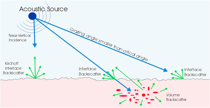
Figure 1. Total backscattering is described as the sum of two processes: interface and volume. Interface contribution can correspond to various scattering regimes depending on incidence angle (and frequency).

In the case of an absorbing second medium, Equation 1 remains valid, by expressing velocity $c_2$ as a complex value, whose imaginary part is linked to the seafloor absorption coefficient. This property of sediments is especially important for modelling the volume backscatter component (see §2.3).

Practically, it is proposed that the ESAB model uses the impedance contrast z as a fundamental and practical interface parameter. However, calculating the transmission angle refracted according to Equation 2 implies using the sound speed ratio c; it is hence helpful to introduce an approximate relationship between c and z, avoiding the need to separate density and sound speed parameters while preserving physical significance and model’s simplicity. Starting from the synthetical results from classical geoacoustic literature (Hamilton, 1974; Hamilton, 1980; Hamilton and Bachman, 1982) the sound-speed contrast $c$ between sediment and seawater can be approximated by a linear relationship with z (see Supplementary Material - Geoacoustical modelling applied in ESAB):

$c=c_2/c_1\approx 0.7030+0.2055z(3)$

The sediment-water impedance contrast $z$ is hence the first input parameter of the ESAB model. In non-dispersive media, it is expected to be independent of frequency.

2.2 Interface roughness

2.2.1 Roughness modelling

The interaction between electromagnetic/acoustic waves and natural surfaces in radar/sonar remote sensing is strongly influenced by interface roughness, which has to be considered relative to the wavelength $\lambda$ (Engman and Wang, 1987), as expressed by the dimensionless roughness parameter at incidence ${\theta }_1$

$g=2k\zeta {\cos \theta }_1(4)$

where $k=2\pi /\lambda$ is the incident signal wavenumber and $\zeta$ is the root mean square (RMS) height of interface elevations around the average depth value. This roughness parameter (aka “Rayleigh parameter”) actually scales the surface physical relief to the signal wavelength.

Large-scale seafloor relief features (i.e., at topographic scale) are to be treated deterministically and are not considered here; for acoustic signal backscatter, the concept of roughness concerns relief scales that cannot be resolved by bathymetry sonar measurements. According to interface roughness magnitude, different reflection/scattering regimes occur, corresponding to various physical models. For rough interfaces ($\zeta$ >> $\lambda$), the wavelength is much smaller than the dominant relief features, so that the interface can be considered as a continuum of apparent “facets” acting like locally plane reflectors (see, e.g., Brekhovskikh and Lysanov, 1982). This is the fundamental concept of the “Facet Method” based on Kirchhoff’s approximation, a geometric approach considering the local interface curvature and assuming that specular reflection occurs then on the locally tangent plane; it is valid for large curvature radii of the interface compared to wavelength and works most effectively for steep incidence angles (Beckmann and Spizzichino, 1963). At the other end of the roughness scale ($\zeta$ << $\lambda$), the interface roughness just infringes small statistical phase perturbations to the incident wavefront; this situation is addressed by the Small Perturbation Method, involving small phase shifts of the incident wave caused by surface roughness and modeled as a stationary function; the main contribution to scattering is then Bragg’s phenomenon. This case corresponds to small values of $g$ and oblique incidences (Rice, 1951; Valenzuela, 1978).

In the model proposed here, the interface scattering component is based on a two-scale approach involving both the facets (or Kirchhoff’s) theory at “small scale” and the small perturbation method (SPM) at “micro-scale”, combined through a physically motivated transition function. The detailed formulation of this transition is given in Section 2.4.2. Following radar literature as well as previous acoustical models (e.g., Jackson et al., 1986), this approach acknowledges that different scattering mechanisms dominate at different roughness scales and angles of incidence, a long-established concept both in radar and sonar remote sensing.

2.2.2 Interface roughness description

As a preliminary to the presentation of the two models, it is useful to establish the relationship between the components of interface roughness, linking its roughness spatial spectrum with the variances of interface slopes and elevations.

The seafloor roughness is characterized by its power spectrum $\mathrm{\Omega }\left(\kappa \right)$ usually written in the form:

$\mathrm{\Omega }\left(\kappa \right)=a^2{\kappa }^{-\gamma }(5)$

where κ is the interface roughness spatial frequency and γ takes values typically between 3.0 and 3.5 (de Moustier and Alexandrou, 1991). The exponent γ directly and strongly influences acoustic backscatter modeling and sonar data interpretation based on the physical characteristics of the seabed. The value γ = 3.5 is often used for natural sedimentary seabed and areas with gradual variations in roughness, while γ = 3 may be more appropriate for rockier seabeds and areas with more uniform roughness scales. The scaling factor $a^2$ gives the magnitude of the elevation distribution corresponding to the roughness spectrum.

The spatial spectrum $\mathrm{\Omega }\left(\kappa \right)$ has to be split in order to address the different roughness regimes. Disregarding its lower-frequency part associated with deterministic large-scale topography, one can consider a medium-frequency part (“small-scale”) adapted to the Kirchhoff’s approach and a high-frequency part (“micro-scale”) associated with the SPM. These two parts split around a transition “cut-off” value κ_C that is not intrinsic to the interface relief alone but also depends on the acoustical frequency. Following Novarini and Caruthers (1994), the cut-off spatial frequency corresponds to the condition that the Rayleigh parameter (i.e., Formula 4 considered at normal incidence) for microroughness equals unity:

$g^2=4k^2{\zeta }_{\mu }^2=16{\pi }^2\frac{f^2}{c^2}{\zeta }_{\mu }^2=1(6)$

Formula 6 makes it possible to obtain the effective ${\zeta }_{\mu }^2$ at a given frequency f. Moreover, the microroughness elevation variance ${\zeta }_{\mu }^2$ is defined as

${\zeta }_{\mu }^2=2\pi {\displaystyle {\int }_{{\kappa }_c}^{{\kappa }_H}}\mathrm{\Omega }\left(\kappa \right)\kappa d\kappa (7)$

and the small-scale facet-slope variance as:

${\delta }_f^2=2\pi {\displaystyle {\int }_{{\kappa }_L}^{{\kappa }_C}}\mathrm{\Omega }\left(\kappa \right){\kappa }^{3}d\kappa (8)$

where κ_L and κ_H are respectively the low- and high-limit values of the spatial frequency spectrum.

Formulas 5-8 will now be used in order to detail the roughness backscatter models, at both scales in a consistent way, as described in the next paragraphs.

2.2.3 Small-scale roughness: the facets model

For the small-scale facet (or Kirchhoff) regime, the backscattering cross-section ${\sigma }_f$ is primarily given (Brekhovskikh and Lysanov, 1982) by the classical formula:

${\sigma }_f\left({\theta }_1\right)=V^2\left(0\right)\exp \left[-{\tan }^2{\theta }_1/\left(2{\delta }^2\right)\right]/\left(8\pi {\delta }^2{\cos }^4{\theta }_1\right)(9)$

where $V^2\left(0\right)$ is the intensity reflection coefficient at normal incidence; the exponential term $\exp \left[-{\tan }^2{\theta }_1/\left(2{\delta }^2\right)\right]/\left(2\pi {\delta }^2\right)$ is a Gaussian distribution depicting the assumed probability distribution of surface slopes, in which the facet-slope variance ${\delta }^2$ controls the distribution width; and the $co{s}^4{\theta }_1$ term accounts for geometric spreading and projection effects.

In this “facets model”, the key parameter is the standard deviation of the facet-slope distribution, which directly controls the angular width of the specular lobe around normal incidence ${\theta }_1$ = 0. Importantly, this model usually assumes a Gaussian distribution of slopes (Brekhovskikh and Lysanov, 1982), which simplifies the mathematical treatment while still providing a reasonable approximation for many natural surfaces¹. The key point of this facets theory is that the seafloor backscatter angular response near normal incidence (typically up to 35°) is proportional to the slope distribution, as the backscatter strength in this region is dominated by facets oriented normally to the transducer location. This relationship between slope statistics and angular response provides a strong physical meaning to the model parameters, allowing for an intuitive interpretation of seafloor characteristics from acoustic data. However, although this is frequently a good approximation, the roughness-slope distribution is not systematically Gaussian, as non-Gaussian angular responses are frequently observed in field data.

It must be emphasized that the relationship between interface-scattering and acoustic-wavelength is fundamental to the model’s physical relevance. In this respect, the variance of the facet-slope distribution has to be scaled by the normalized frequency, reflecting a key insight about rough-interface scattering: for a given sonar configuration, the backscatter effectively corresponds to only fractions of the full distributions of slopes and elevations, limited both by the sonar footprint extent on the interface and by the frequency-scaled roughness. This wavelength-dependent filtering effect has been well documented in previous research works (Novarini and Caruthers, 1998; Shaw and Smith, 1990) demonstrating that acoustic backscatter is mostly sensitive to roughness components with scales comparable to the acoustic wavelength. Using both the existing theories and the experimental data from our Concarneau dataset (Fezzani et al., 2025), we tried to determine frequency-scaling factors in order to minimize the frequency dependence of the derived roughness parameters. This approach (also applied here below to the volume backscatter contribution) makes it possible for our ESAB model to extract physically meaningful seabed parameters that remain consistent across the operational frequency range of typical seafloor-mapping sonars.

In order to build the ESAB model, it is now proposed to improve the classical and widely accepted expression of the facets model on three important points, often disregarded:

2.2.3.1 The effective size of the facets (and hence the statistics of their local slopes) is dependent on frequency

This phenomenon is very clearly and commonly observed on experimental data: the typical bell-shaped central lobe around normal incidence both widens and decreases when frequency increases, as illustrated in Figure 2. Since the classical facets formula 9 does not provide such a trend, it is suggested here to account for a frequency dependence of the effective roughness slopes.

Figure 2

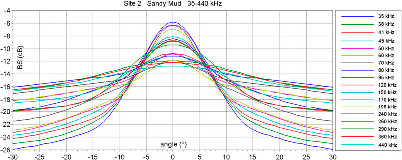
Figure 2. Experimentally-measured frequency dependence of the Angular Response Curves main lobe. The graph displays backscatter strength (dB) versus incidence angle (±35°) measured at various frequencies from 35 kHz to 440 kHz at Site 2 (Sandy Mud). These results clearly illustrate a systematic trend: the main lobe widening with increasing frequency, together with a peak level decrease at nadir, with a general increase at oblique incidence.

The frequency dependence of the facet-slope variance ${\delta }^2\left(f\right)$ can be obtained from Equation 8, after obtaining κ_c from Equations 6–7 at a given frequency f. These developments result in the following expression:

${\delta }^2\left(f\right)=D_1{f}^{D_2}(10)$

where $D_1$ and $D_2$ are constants that solely depend on the seafloor roughness power spectrum $\mathrm{\Omega }\left(\kappa \right)$ defined in Equation 5:

$D_1=\frac{2\pi }{4-\gamma }{a}^{D_2+1}{\left[\frac{32{\pi }^3\left(\gamma -2\right)c^2}{\left(\gamma -2\right)c^2}\right]}^{D_2}\text{and}{D}_2=\frac{8-2\gamma }{\gamma -2}$

Hence the facet-slope variance ${\delta }^2\left(f\right)$ is proportional to frequency at power $D_2$ defined by the spectrum exponent $\gamma$; this frequency dependence is applied in the ESAB model.

In order to define a practical roughness parameter independent of frequency, ${\delta }^2\left(f\right)$ can be expressed using a reference frequency f₀ and a proportionality coefficient s²:

${\delta }^2\left(f\right)=s^2{\left(f/f_0\right)}^{D_2}\text{with}{s}^2=D_1{f}_0^{D_2}(11)$

where s @ f₀ is actually the RMS facet slope normalized at frequency f₀; it is an intrinsic characteristic of the local seafloor roughness and then usable as a descriptor for classification.

It is interesting to illustrate Equation 10 by particular values of the roughness spectrum exponent varying between 3.0 and 3.5, showing the dependence of the facet-slope variance:

• γ = 3.00 ${\delta }^2\left(f\right)\sim f^{2.0}$

• γ = 3.25 ${\delta }^2\left(f\right)\sim f^{1.2}$

• γ = 10/3 $\approx$ 3.333 ${\delta }^2\left(f\right)\sim f$

• γ = 3.50 ${\delta }^2\left(f\right)\sim f^{0.667}$

Note in particular the case $\gamma =10/3\approx 3.333$ for which the facet-slope variance is simply proportional to frequency, while this value is a good intermediate inside the interval [3–3.5]. It is proposed here to use it as a practical default value when the spectrum shape is not known and cannot be extracted from the experimental data.

2.2.3.2 The facets reflection coefficient is affected by the facets microroughness

The imperfect smoothness of facets causes a loss of coherence (and hence of average intensity) of the reflected signals. This imperfection is intrinsic to the interface configuration: facets are fragments of continuously curved surfaces, and hence they are not strictly plane in general cases. Moreover, and at a smaller scale, the granular nature of the sediment causes a microroughness to be present on the interface, linked to the grain size distribution. Hence, the wave reflection by a facet is affected by an effect of coherence loss, leading to an average intensity loss expressed as $\exp \left(-4k^2{\zeta }^2{\cos }^2\theta \right)$ that must be incorporated into the expression of the facets backscatter cross-section. This was named the “rough facet” regime by Novarini and Caruthers (1994), who showed that the maximal effective magnitude of this extra-loss corresponds to the value $g_{\mu }=1$, hence a multiplicative factor $\exp \left(-1\right)\sim 0.368$ i.e., −4.343 dB. The important point is that this is taken as the limit condition for a facet to exist; said otherwise, beyond this point the facet does not play its role of a plane reflector anymore, and hence this defines the limit size of facets. This coherence loss due to the imperfect smoothness of the facets is applied in ESAB both through the extra-loss term and in order to define the facets extent and slope.

2.2.3.3 The hypothesis of a Gaussian distribution of slopes must be relaxed in order to include other statistical forms

Although classically admitted for current applications of the facets model, the Gaussian character of the interface slope distribution should rather be considered a canonical case. Actually, the main result of the facet theory (namely, the backscatter cross-section proportionality to the slope distribution) is a very strong assessment since the measured angular dependence of backscatter (at least in the facets regime, i.e., from normal to moderately steep angles) reproduces the roughness slope distribution. Hence, measuring a non-Gaussian shape for the BS angular dependence implies that the slope distribution also follows this non-Gaussian behavior.

However, most experimental results show that angular response curves (or ARCs) are usually peak- or bell-shaped, with a maximum at normal incidence and a fast decrease on both sides, although with various fall-off behaviours (see Fezzani et al., 2025) - either exponential, or linear, or even with a sudden change of slope. However, it can be shown that these various peaked behaviors of ARCs can be efficiently approximated by a simple sum of two normal laws with different width and height. Hence, it is proposed here to express the facets backscatter cross-section as a summation of two Gaussian components with two different facet-slope variances ${\delta }_1^2$ and ${\delta }_2^2$ :

${\sigma }_f\left({\theta }_1\right)={\sigma }_{f1}\left({\theta }_1\right)+{\sigma }_{f2}\left({\theta }_1\right)(12)$

This dual-Gaussian model (Formula 12) is illustrated in Figure 3, which displays acoustic backscatter ARCs for various seafloor substrates. The blue curves represent measured backscatter strength at 45 kHz as a function of incidence angle on four seafloor types, while the red curves represent the sum of two Gaussian distributions fitted to the measured angular responses. Each distribution has zero mean but different standard deviations (displayed as STD1/STD2). Site 1 (Sandy Mud) exhibits a narrower distribution (STD1 = 7.2) compared to Site 2 (Muddy Gravelly Fine Sand, STD1 = 11.7). Site 6 (Maërl) shows a triangular-shaped response pattern with small STD1 (2.7) and large STD2 (15.6), suggesting a bimodal distribution of surface slopes. In contrast, Site 7 (Bedrock) shows an angular response that can be modeled by a single Gaussian distribution (STD1 = STD2 = 18.5). These observations support the hypothesis that, while the backscatter angular response near normal incidence reproduces the seafloor roughness slope histogram, a dual-Gaussian model can capture the diversity of angular backscatter patterns observed across different substrate types.

Figure 3

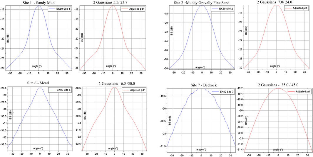
Figure 3. EK80-measured Angular Response Curves for various seafloor substrates at steep angles. The blue curves represent measured backscatter strength at 45 kHz as a function of incidence angle across four distinct seafloor types. The red curves represent the two-Gaussian combination that was fitted to the measured ARCs.

The facet-slope variance ${\delta }_1^2$ is another key parameter to be obtained from the ESAB inversion, summarizing the interface roughness properties. However, as discussed above, its effective values are frequency dependent; therefore, the roughness parameter to consider will actually be its reference values $s_1^2$ at a normalizing frequency f₀ as expressed in Equation 11. Note that the facet-slope variance ${\delta }_2^2$ of the second Gaussian component and the power spectrum exponent $\gamma$ can be extracted as intermediate parameters of the model, usable, e.g., for more detailed analyses of the roughness.

Note - The reference frequency f₀ introduced above is needed for expressing the frequency dependence of the roughness quantities; a similar normalization will be applied for volume scattering presented in §2.3. Considering that the typical average magnitude of the physical features causing seafloor scattering for echosounders is the centimeter, whether for the interface roughness or for volume inhomogeneities, it is proposed here to define a reference unit wavelength of $\lambda$₀ = 1 cm = 10^–2 m, corresponding to a frequency f₀ = 150 kHz for the canonical velocity value 1,500 m/s. This reference value is also representative of the frequency range of many echosounders, especially for medium-deep and shallow waters.

2.2.4 Micro-scale roughness: the Bragg model

At the micro-roughness scale, the backscatter component generated by the interaction between the acoustical wave and the interface roughness is dominated by the “Bragg effect” resulting from the resonance between the incident acoustical wavelength projected on the interface and the corresponding spatial frequency spectrum of the interface relief (Thorsos and Jackson, 1989). For one signal frequency and incidence angle, the obtained backscatter cross-section is classically expressed (e.g., Novarini and Caruthers, 1998) as:

${\sigma }_B\left({\theta }_1\right)=\frac{V^2\left({\theta }_1\right)}{{\pi }^2}{k}^4\text{co}{\mathrm{s}}^4{\theta }_1\mathrm{\Omega }\left(\frac{k}{\pi }\sin {\theta }_1\right)(13)$

using the same notations as above.

When assuming (as in Equation 5) a negative-exponential roughness spectrum $\mathrm{\Omega }\left(\kappa \right)=a^2{\kappa }^{-\gamma }$, a direct analytical relationship can be found between the roughness-slope standard deviation and the RMS roughness elevation. This property is particularly valuable in our case since it allows the expression of the Bragg scattering component without the need to introduce an additional independent roughness parameter for this particular regime. This simplification respects the theoretical integrity of the model while reducing its parametric complexity, making it more practical for inversion problems and preserving its physical meaning.

Using the relationships established above between ${\delta }^2\left(f\right)$ and ${\zeta }_{\mu }^2$, the micro-scale backscatter cross-section given by Equation 13 can be developed into a function of the facet-slope variance ${\delta }_1^2$ alone:

${\sigma }_B\left({\theta }_1\right)=D_3{V}^2\left({\theta }_1\right)\frac{\text{co}{\mathrm{s}}^4{\theta }_1}{\text{si}{\mathrm{n}}^{\gamma }{\theta }_1}{\left({\delta }_1^2\right)}^{D_4}(14)$

with:

${D_3=2}^{\gamma -5}{\pi }^{\gamma -3}{\left(4-\gamma \right)}^{D_4}{\left(\gamma -2\right)}^{{1-D}_4}{D}_4=\frac{\gamma -2}{2}$

This microroughness component ${\sigma }_{\mu }$ shows a characteristic angular dependence proportional to $\text{co}{\mathrm{s}}^4{\theta }_1/\text{\hspace{0.5em}si}{\mathrm{n}}^{\gamma }{\theta }_1$, leading it to strongly diverge at vertical incidence (in ${1/\text{si}{\mathrm{n}}^{\gamma }\theta }_1$), and to rapidly decrease at grazing angles (in ${\text{co}{\mathrm{s}}^4\theta }_1$); hence its practical influence is restricted to intermediate oblique angles. It also depends, as expected, on the interface reflection coefficient, on frequency, and on the roughness spectrum reference power. Practically, for numerical implementation the divergence around vertical incidence has to be controlled by a dedicated weighting term (see §2.4.2 below).

This microroughness backscatter component ${\sigma }_{\mu }$ can interestingly be expressed for particular values of the spectrum exponent $\gamma$ resulting in some simplification:

• $\gamma =3.0$ ${\sigma }_B\left({\theta }_1\right){\sim V}^2\left({\theta }_1\right)\frac{\text{co}{\mathrm{s}}^4{\theta }_1}{\text{si}{\mathrm{n}}^3{\theta }_1}{\left({\delta }_1^2\right)}^{0.5}$

• $\gamma =3.25$ ${\sigma }_B\left({\theta }_1\right)\sim V^2\left({\theta }_1\right)\frac{\text{co}{\mathrm{s}}^4{\theta }_1}{\text{si}{\mathrm{n}}^{3.25}{\theta }_1}{\left({\delta }_1^2\right)}^{0.625}$

• $\gamma =3.333$ ${\sigma }_B\left({\theta }_1\right)\sim V^2\left({\theta }_1\right)\frac{\text{co}{\mathrm{s}}^4{\theta }_1}{\text{si}{\mathrm{n}}^{3.333}{\theta }_1}{\left({\delta }_1^2\right)}^{0.667}$

• $\gamma =3.5$ ${\sigma }_B\left({\theta }_1\right)\sim V^2\left({\theta }_1\right)\frac{\text{co}{\mathrm{s}}^4{\theta }_1}{\text{si}{\mathrm{n}}^{3.5}{\theta }_1}{\left({\delta }_1^2\right)}^{0.75}$

2.3 Sediment volume scattering

The sediment volume backscatter cross-section is modelled here using formula (3.75) in (Lurton, 2010):

${\sigma }_V=\frac{m_V}{4\beta }{\left|1-V^2\left({\theta }_1\right)\right|}^2{\left(\frac{c_2}{c_1}\right)}^2\frac{{{\cos }^2\theta }_1}{\cos {\theta }_2}(15)$

where $m_V$ is the “volume scatter parameter” associated to a unit volume, and β is the sediment absorption coefficient expressed as an amplitude exponential decrement (in Np/m). The volume parameter $m_V$ is the backscatter cross-section associated to a unit volume of sediment (including a frequency dependence discussed below). The factor 1/4β defines the conventional extinction depth of the sound wave inside the sediment, hence determining the effective scattering volume considered from the interface. ${\left|1-V^2\right|}^2$ is the combined two-way intensity transmission factor across the water-sediment interface. Finally, ${\left(\frac{c_2}{c_1}\right)}^2\frac{{{\cos }^2\theta }_1}{\cos {\theta }_2}$ comes from the modification of the divergence loss of a sound beam crossing the water-sediment interface.

The frequency dependence of the volume backscatter component comes from both the attenuation coefficient β and from the volume parameter $m_V$. The attenuation coefficient is usually admitted being roughly proportional to frequency (Hamilton, 1980) and hence often expressed in dB per wavelength; this hypothesis will be retained here. Regarding the volume parameter, it is proposed here to express it in the form $m_V=m_0{\left(\frac{f}{f_0}\right)}^n$ where $m_0$ is the reference value at f₀, and n is the exponent of the frequency dependence (expected to stay below 4 corresponding to the extreme case of Rayleigh scattering). The combination of both terms (β and $m_V$) finally leads to a frequency dependence of ${\sigma }_V$ in $f^{n-1}$. Practically, the exponent n value is best determined heuristically. A previous dedicated experiment and synthesis (Fezzani et al., 2021) of backscatter measurements vs. angle and frequency gave values of (n-1) ranging between 0.6 and 0.7 for frequencies varying from 45 to 450 kHz. From this result it is suggested here to retain an intermediate value of 1.65 for n, averaged over a variety of different types of sediment (Figure 4). It is clear that different numerical values could be obtained from other configurations; hence, it is acknowledged that this particular value (today applied in ESAB) is not expected to give more than a reasonable magnitude of the frequency dependence. The ESAB parameter μ used in the model inversion is actually the value of $m_0$ expressed in decibels, specifically: $\mu =10\text{\hspace{0.17em}lo}{\mathrm{g}}_{10}\left(m_0\right)$, where $m_0$ is the volume backscatter parameter normalized at the reference frequency f₀ = 150 kHz.

Figure 4

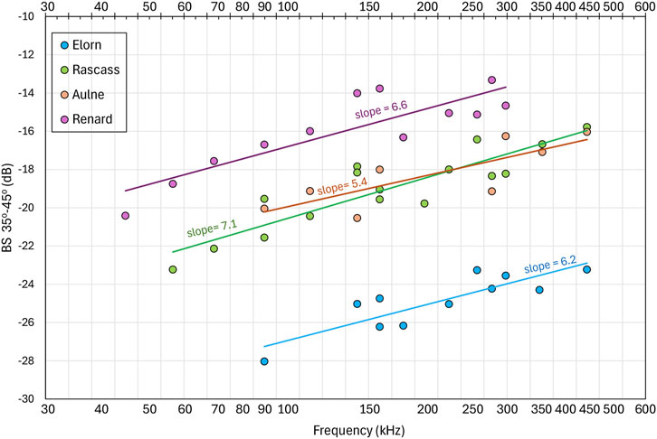
Figure 4. Variation with frequency of the mean oblique backscatter strength (BS, averaged between 35° and 55°) over four sites: Elorn, Aulne, Rascass, and Renard (Fezzani et al., 2021). The x-axis represents frequency both in kHz and in logarithmic scale, while the y-axis represents mean oblique BS in decibels. Linear trends with their slope values are plotted for each site, specifying the frequency dependence expected to increase mainly due to volume scattering. The measured slopes varied between 0.6 and 0.7, and an average value of 0.65 was used as the frequency exponent for the volume scattering in the ESAB model.

2.4 Synthesis and direct computation application

2.4.1 Synthetic form

Finally, the ESAB backscattering strength (Equation 16) combines both interface (${\sigma }_I$) and volume (${\sigma }_V$) contributions before converting their intensity summation to decibels:

$BS\left({\theta }_1,f\right)=10\text{\hspace{0.5em}lo}{\mathrm{g}}_{10}\left[{\sigma }_I\left({\theta }_1,f\right)+{\sigma }_V\left({\theta }_1,f\right)\right](16)$

where each term comes from Equations 12-15 and accounts for the various improvements, simplifications and approximations presented and discussed in the sections above. All these terms are now explicitly dependent on frequency.

As a reminder from the previous paragraphs, it must be emphasized that this final formulation (Equation 16) only requires four input parameters related to the seafloor configuration: the water-sediment impedance contrast z; the sediment volume scattering strength parameter μ; and the two interface roughness facet-slope standard deviations ${\delta }_1$ and ${\delta }_2$.

2.4.2 Transition terms

The transition between the two roughness scattering regimes (facets and Bragg) presented above is managed through a simple sigmoid angle-dependent function (Equation 17) featuring a frequency-dependent crossing angle. This ensures physical continuity between the two regimes and hence better represents the overall seafloor scattering behavior. As proposed in (Mourad and Jackson, 1989), a crossing angle ${\theta }_x$ can be defined by ${\sigma }_{f1}$ (Equation 9) dropping by −15 dB from its normal incidence value ${\sigma }_{f1}\left(0\right)$. The weighting function writes:

$\mathrm{\Sigma }\left({\theta }_1\right)=1/\left[1+\exp \left(-180/\pi \left({\theta }_1-{\theta }_x\right)\right)\right](17)$

where ${\theta }_1$ and ${\theta }_x$ are expressed in radians.

The resulting form of the interface roughness scattering ${\sigma }_{Is}$ (featuring the sigmoid weighting) is finally expressed in Equation 18. Note that, before being combined with ${\sigma }_{f1}$ through the sigmoid (Equation 17), ${\sigma }_{f2}$ is summed with ${\sigma }_B$, as both are triggered beyond the crossing angle ${\theta }_x$.

${\sigma }_{Is}\left({\theta }_1\right)={\left[\sigma \right.}_B\left({\theta }_1\right)+{\sigma }_{f2}\left({\theta }_1\right)]\mathrm{\Sigma }\left({\theta }_1\right)+[1-\mathrm{\Sigma }\left({\theta }_1\right)]{\sigma }_{f1}\left({\theta }_1\right)(18)$

The ESAB model uses a second sigmoid function in order to reduce the volume scattering contribution near normal incidence, complementing the constrained model inversion approach (Section §3) where all parameters (z, ${\delta }_1$, ${\delta }_2$, $m_0$) are bounded within physically meaningful ranges typical of seafloor sediments. At normal incidence, both decreasing roughness and increasing impedance contrast can produce higher backscatter strength, creating an inherent ambiguity (Figures 5A,C). Without sigmoid weighting, adding volume scattering in this angular region could lead the inversion process to converge on parameter combinations that, while mathematically valid, would violate physical expectations for seafloor properties. By effectively separating the angular domains where different scattering mechanisms predominate (Fonseca and Mayer, 2007), the sigmoid weighting allows the interface parameters (z, ${\delta }_1$, ${\delta }_2$) to be primarily determined from near-nadir returns ($\theta$ <$\left.{\theta }_v\right)$, while the volume parameter $m_0$ is mainly controlled by oblique angle responses ($\theta$ >$\left.{\theta }_v\right)$, improving the numerical stability of the simulated annealing inversion process (see §3.1.1). A limit angle value of ${\theta }_v$ = 0.1745 radians (or 10^o) was found appropriate for the inversion process. The division by 2 forces a smoother transition in the sigmoid. The volume backscatter cross-section featuring the sigmoid term finally writes:

${\sigma }_{Vs}\left({\theta }_1\right)={\sigma }_V\left({\theta }_1\right)/\left(1+\exp \left(-180/\pi \left({\theta }_1-{\theta }_v\right)/2\right)\right)(19)$

Figure 5

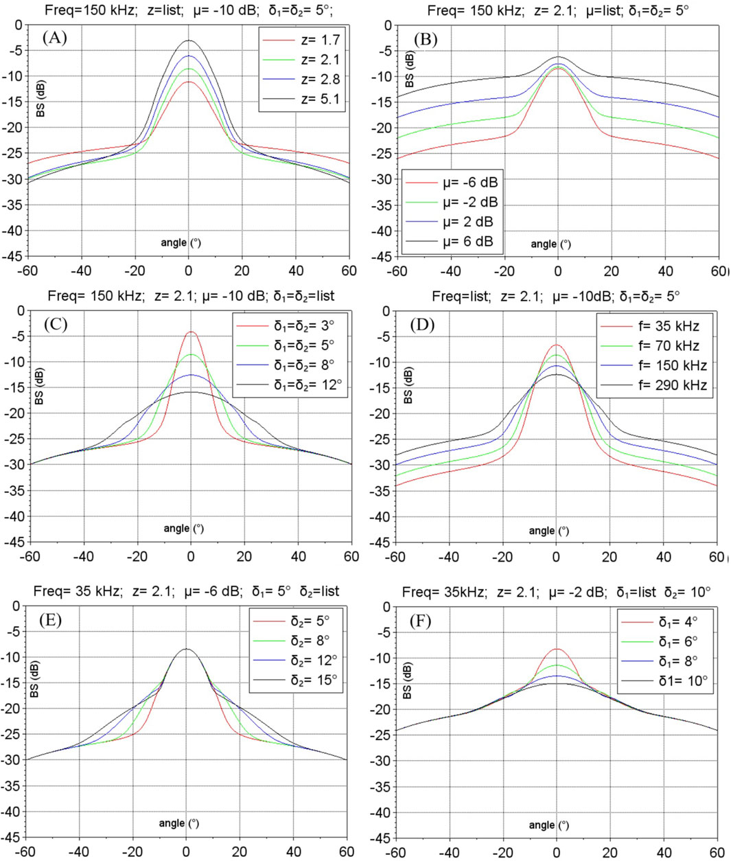
Figure 5. Direct modeling simulation results (in dB) as a function of the incident angle (in °) (A) f = 150 kHz, varying only the impedance contrast: z = [1.7, 2.1, 2.8, 5.1], with $\mu$ = −10 dB and ${\delta }_1$ = ${\delta }_2$ = 5°; (B) f = 150 kHz, varying only the volume parameter: $\mu$ = [-6 dB, −2 dB, 2 dB, 6 dB ], with z = 2.1, ${\delta }_1$ = ${\delta }_2$ = 5°; (C) f = 150 kHz; varying both roughness parameters: ${\delta }_1$ = ${\delta }_2$ = [3°, 5°, 8°, 12°], with z = 2.1; $\mu$ = −10 dB; (D) varying only the frequency: f = [35 kHz, 70 kHz, 150 kHz, 290 kHz], with z = 2.1, $\mu$ = −10 dB, ${\delta }_1$ = ${\delta }_2$ = 5°; (E) f = 35 kHz; varying just ${\delta }_2$ = [ 5°, 8°, 12°, 15°], with z = 2.1; $\mu$ = −6 dB; ${\delta }_1$ = 5°; (F) f = 35 kHz, varying just ${\delta }_1$ = [4°, 6°, 8°, 10°], with z = 2.1, $\mu$ = −2 dB; ${\delta }_2$ = 10°.

The final expression for the ESAB backscatter strength is given in Equation 20; it includes the interface and volume components corrected by the sigmoid functions presented above.

$BS\left({\theta }_1\right)=10\text{\hspace{0.5em}lo}{\mathrm{g}}_{10}\left[{\sigma }_{Is}\left({\theta }_1\right)+{\sigma }_{Vs}\left({\theta }_1\right)\right](20)$

Although these transition terms are, strictly speaking, out of the physical modelling, they are of paramount importance for the numerical stability of the model, especially when applying it to inversion purposes.

2.4.3 Direct computation examples

The simplified adaptation of both sonar- and radar-inspired modeling techniques presented above is expected to provide a comprehensive description of seafloor backscattering while ensuring computational efficiency, minimizing the formal complexity (including the input physical parameters) and flexibly, and preserving physical consistency across different angular and frequency regimes. The model versatility makes it able to represent a wide range of seafloor types through appropriate parameter selection, while its theoretical foundation in scattering theories justifies its relevance and ensures robust physical behavior.

A major interest of direct backscattering computations is the demonstration (see, e.g., Figure 5) of how each parameter distinctly affects the angular response, making possible a clear phenomenological interpretation of intricate processes. The impedance contrast z primarily influences backscatter level near normal incidence; this is illustrated in Figure 5A, where increasing z from 1.3 to 4.1 produces significantly stronger returns (+13 dB) in the specular lobe while maintaining comparable responses (within 3 dB) at oblique angles. Notably, this enhancement of normal incidence backscatter by increasing impedance is similar to the effect of decreasing surface roughness, through different physical mechanisms (Figure 5C). The volume parameter μ shows opposite behavior (Figure 5B), mainly affecting oblique angles (>30°) with minimal impact on near-nadir returns (where it has been, by the way, minimized by the sigmoid weighting). The facet-slope standard deviations (${\delta }_1$ and ${\delta }_2$) shape the overall angular response: increasing ${\delta }_1$ reduces the specular peak while broadening the angular distribution, a characteristic property of diffuse scattering from small-scale roughness. Meanwhile and as expected from its introduction and justification, ${\delta }_2$ more strongly influences the response beyond 20° incidence angles (Figures 5E,F) and significantly departs the overall angular response from the canonical Gaussian shape. Interestingly, the red curve (z = 1.7) in Figure 5A shows higher backscatter at oblique angles due to the impedance-dependent attenuation model. Low impedance ratios result in lower attenuation coefficients, allowing deeper acoustic penetration and enhanced volume scattering contributions, which dominate the oblique-angle response and produce the elevated off-nadir backscatter seen in this curve.

The frequency dependence shows behavior similar to roughness variation since the model uses the classical Rayleigh parameter, which relates wavelength and surface roughness (Equation 4). At the lowest frequencies, the angular response shows a pronounced specular lobe with rapid decay at oblique angles (Figure 5D). As frequency increases, the angular response broadens and the specular component diminishes. Unlike pure interface roughness dependence, the frequency increase also enhances volume scattering, which scales with the $k_0^{0.65}$ term discussed in §2.3, demonstrating how the model captures the distinct frequency dependence of surface and volume scattering mechanisms.

2.4.4 From GSAB to ESAB

A predecessor to the ESAB presented here, the Generic Seafloor Acoustic Backscatter (GSAB) model (Lamarche et al., 2011) already proposed a more practical approach aiming at a functional description of the main backscatter regimes (near-specular lobe, oblique-angle plateau and grazing-angle fall-off) using simple mathematical expressions and a limited set of six input parameters (possibly only four significant ones), and effectively fitting a majority of backscatter ARCs. The GSAB model comprises three components: a normal law $A\exp \left[-{{\theta }_1}^2/\left(2B^2\right)\right]$ describing near-specular reflection; a powered-cosine component $C\text{\hspace{0.17em}co}{\mathrm{s}}^D{\theta }_1$ for the backscatter plateau and fall-off; and a second normal law $E\exp \left[-{{\theta }_1}^2/\left(2F^2\right)\right]$ effective at intermediate angle regimes. While really practical and versatile for empirical data fitting, the GSAB parameters lacked direct physical interpretation leading to quantified seafloor properties, and missed an explicit frequency dependence (in the sense that each frequency needs one specific parameter set).

ESAB builds upon the GSAB’s functional approach while providing clear physical interpretation through a small number of parameters representing three fundamental seafloor properties: acoustic impedance for water-sediment contrast; slope values for interface roughness; and a volume scattering parameter for sediment inhomogeneity. This limitation to a remarkably low number of input parameters was obtained by using ad hoc relationships linking the various factors involved in the physical processes.

Moreover, unlike GSAB, the ESAB model incorporates explicit frequency dependence of interface and volume scattering phenomena, defining sediment intrinsic physical properties valid across frequencies. Applied to the Concarneau dataset (Figure 6), ESAB demonstrates physical consistency at 70 and 290 kHz with stable impedance values for sandy mud (z = 1.72) and medium sand (z∼1.90), while GSAB parameters expectedly show greater variability between frequencies. (See Supplementary Material - Comparison of GSAB and ESAB).

Figure 6

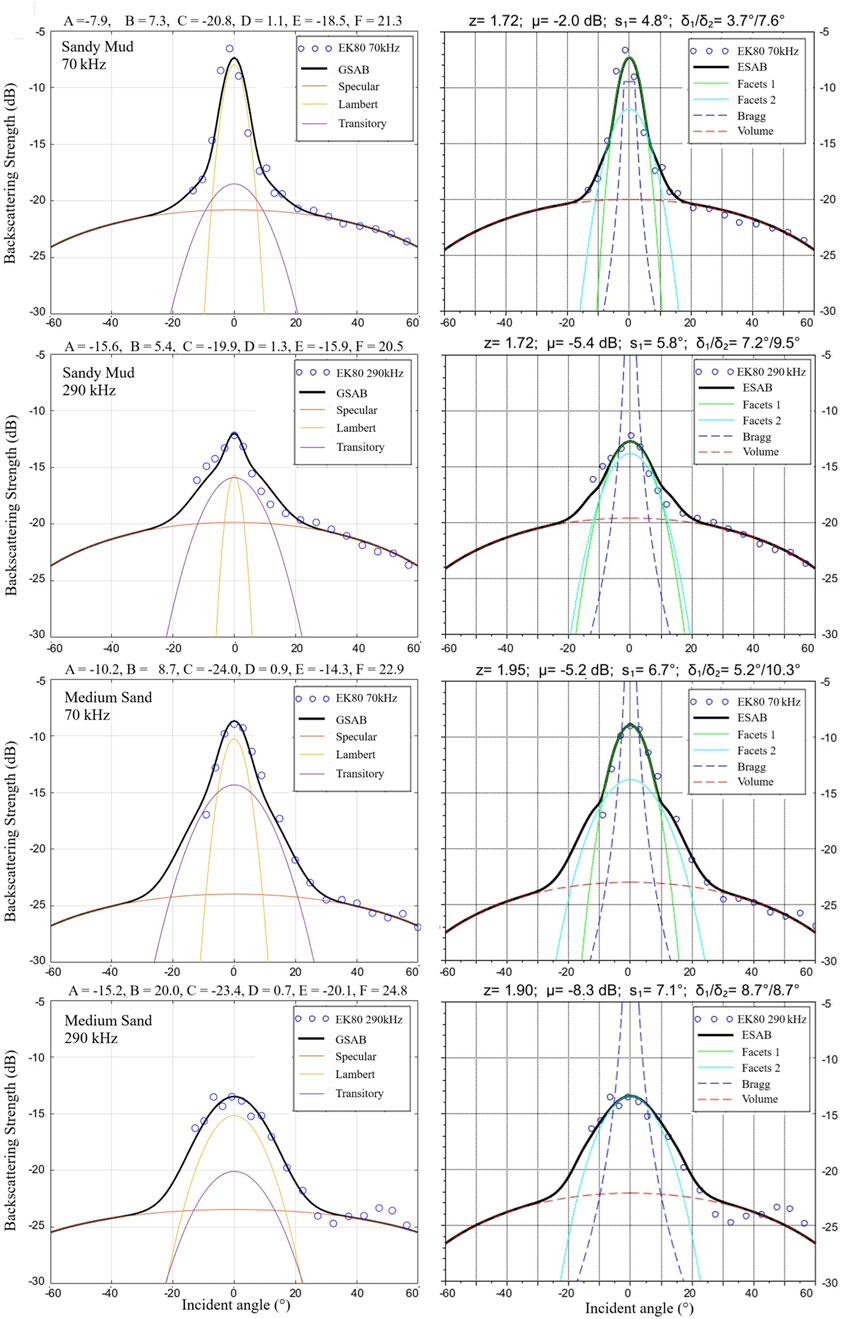
Figure 6. Comparison between GSAB and ESAB inversion results at 70 kHz and 290 kHz for two distinct seafloor types (Sandy Mud and Medium Sand). Notice that both models decompose the angular response into similar mathematical components. However, differently from GSAB parameters, ESAB parameters show physical consistency at the two frequencies, particularly in the impedance values (z = 1.72/1.72 for Sandy Mud and z = 1.95/1.90 for Medium Sand).

Despite its intrinsic limitations compared to ESAB, the GSAB model still features interesting properties. Its excellent versatility in fitting very different ARC shapes makes it very useful for a parametric description of backscatter; the resulting parameters, although not directly physically interpretable as in ESAB, are however usable for some seafloor type classification or backscatter map segmentation. Moreover, GSAB is still usable for data obtained from non-calibrated echosounders, provided that the result interpretation bears only on parameters not depending on absolute levels: for instance, the specular lobe apertures (B or F); or the grazing angle decrement (D); or the contrast between levels at specular (A) and at oblique (C); all these are expected to be efficient descriptors of the seafloor type. Finally, GSAB can be used as a preliminary analysis tool to be applied before a full ESAB inversion for (1) preconditioning the ARCs under an averaged smoothed shape, and (2) possibly pre-selecting data from seafloor configurations found to be ill-adapted to ESAB.

Note that the final inversion results presented in Section 3 (Figure 8) used GSAB-fitted curves rather than the sparse experimental data points shown in Figure 6. The GSAB fitting provides complete angular response curves covering all angles, which better represent typical multibeam echosounder data that continuously samples the entire angular range. This approach allows the same simulated annealing procedure to be applied to both single-beam and multibeam datasets.

3 Model inversion and analysis of the concarneau dataset

3.1 Numerical inversion process description

3.1.1 Model implementation

The ESAB model implementation follows a structured approach that computes each scattering component separately before combining them into the total backscatter response. The algorithm operates on input angles and includes safeguards against numerical singularities. The implementation calculates reflection and transmission coefficients using Snell’s law with the sound speed ratio relationship given in Equation 3. For the interface scattering components, facet contributions at both scales (${\sigma }_{f1}$ and ${\sigma }_{f2}$) are computed using frequency-dependent slope variances following (Equation 11). The roughness effect on reflection is incorporated through the coherence loss factor 1/e discussed in Section 2.4.2.

The Bragg scattering component is considered at oblique angles, with special handling of near-normal incidences to avoid mathematical singularities. The transition between facet- and Bragg-dominated regimes is managed through a crossing angle (${\theta }_x$) determined by the specular lobe width at −15 dB. This transition is implemented using the sigmoid function described in Equation 17. Volume scattering follows the formulation in Equation 15, with frequency-dependent attenuation, again calculated from impedance-based relationships. An optional sigmoid function (Equation 19) reduces volume contribution near normal incidence, ensuring stable inversion convergence by separating the angular domains where different mechanisms dominate.

The optimization cost function uses a weighted RMS approach, with additional emphasis on near-nadir angles (0°–20°) to enhance the accuracy of interface parameter determination. Parameter constraints are enforced throughout the optimization process, ensuring physical realism by maintaining impedance within realistic bounds (1.0–14.0), volume backscatter parameter between −15 dB and +15 dB, and enforcing the condition ${\delta }_2>{\delta }_1$. The roughness parameters are bounded according to frequency-dependent limits that reflect physical constraints on surface slopes.

The ESAB model inversion uses simulated annealing optimization to determine the three physical parameters (z, μ, s₁) and two distribution parameters (δ₁, δ₂) by fitting theoretical angular response curves to measured backscatter data. This optimization technique, inspired by metallurgical annealing processes (Kirkpatrick et al., 1983), can escape local minima through a so-called “temperature” parameter that gradually decreases, making it suitable for, e.g., the multimodal nature of seafloor parameter inversion. The present implementation uses an initial temperature of T = 0.1, N_c = 15 cooling cycles, and 10,000 iterations per cycle, with temperature decreasing according to T/log₂(1+n_c), where n_c is the current cycle number from 1 to N_c. Parameter perturbations follow normal distributions with controlled scaling to ensure efficient exploration of the solution space while respecting physical constraints. The acceptance probability of the fitting process follows the Metropolis criterion (Metropolis et al., 1953), allowing occasional acceptance of suboptimal configurations to escape local minima and explore the broader solution space.

3.1.2 Model inversion and intermediate parameters

One of the objectives in building ESAB was to keep the number of model’s parameters as low as possible, in order to facilitate the inversion from experimental data, and to classify the seafloor types. In the latter respect, the objective is a classification along only three parameters: impedance ratio, roughness parameter and volume parameter.

The parameter inversion process uses a two-step approach to determine the optimal roughness spectrum exponent γ. First, a model inversion is performed for all seven sites across 18 frequencies using γ = 10/3 ≈ 3.333, which ensures a linear dependence between slope variance and frequency (see Section 2.2.3). After obtaining the inversion results, the frequency dependence of ${\delta }_1$ is analyzed and a residual slope in the regression of $\log {\delta }_1$ against $\log f$ is determined for each sediment site (Sites 1–5). An average residual exponent e₁ is determined, and since ${\delta }_1^2$ is proportional to $f^{2e_1}$, this value is used to calculate the corrected γ through the relationship $\gamma =\left(8+2e_1\right)/\left(e_1+2\right)$, derived from Equation 10. This analysis yielded here γ = 3.508.

A. Sediment bulk properties

Regarding the sediment properties, the model hypothesizes a viscous fluid medium that can be described using three parameters (density, velocity, absorption). However, the model inversion only uses one parameter (impedance, i.e., the density-velocity product); the three original parameters have to be retrieved from geoacoustic considerations (see Supplementary Material - Geoacoustical modelling applied in ESAB), and can be obtained as intermediate results of the inversion process.

B. Interface roughness

Regarding roughness, the classical theories (“facets” and “small perturbations”) explicitly need several input parameters, namely, the reflection coefficient and the variances of roughness slopes and elevations. Following the works by Novarini and Caruthers (1994), Novarini and Caruthers (1998) we have expressed these two roughness variances as frequency-dependent quantities, both defined by the roughness power spectrum that is mainly controlled by the exponent $\gamma$. The cut-off frequency separating the “facets” and “Bragg” regimes is defined by the Rayleigh parameter equalling one. Hence, for a given $\gamma$ value, all the other quantities can be obtained. A practical difficulty is to invert the $\gamma$ value together with the other parameters. The strategy proposed here is to process the inversion in several steps:

1. Fix the $\gamma$ value at one arbitrary value, e.g., 10/3 (see §2.2.4). Run the inversion until obtaining the s₁ parameter as a function of frequency

2. Since s₁ is expected to be constant with frequency, estimate the residual slope and the actual value of $\gamma$.

3. After setting the $\gamma$ value at its correct value, run again the inversion algorithm.

Of course, $\gamma$ can be extracted as another intermediate parameter; it is possibly an interesting descriptor of the local roughness.

C. Sediment volume

The volume backscatter model used in ESAB (Equation 15) features the water-sediment transmission coefficient, the absorption coefficient, and the volume scattering parameter. Since the latter one is expected to be frequency dependent while a constant quantity is desired, this dependence is a priori described by a power of frequency that is here taken equal to an average value extracted from the analysis by Fezzani et al. (2021). The other model parameters are available from the geoacoustical modelling. Finally, the quantity extracted from the model inversion is the volume backscatter parameter μ normalized at frequency f₀.

3.2 Dataset presentation

We present in this section the application of the ESAB model to the inversion of a dataset of calibrated backscatter recordings, acquired within the framework of a multi-year program of data acquisition campaigns conducted across various coastal zones of the French continental shelf (Fezzani and Berger, 2018). These acquisitions were conducted using single-beam echosounders calibrated according to the standard protocol developed for fisheries acoustics (Demer et al., 2015).

A dedicated cruise was conducted (2023) in the Bay of Concarneau (Brittany, France), a region known for its diverse and complex sedimentary environments (Figure 7A) ranging from soft mud deposits in depressions to coarse biogenic maërl beds on elevated terraces (Ehrhold et al., 2006; Ehrhold et al., 2007). This well-documented area was chosen both for its rich variety of seafloor types and for logistical advantages. The primary objective of the cruise was to collect multi-angle multi-frequency datasets over seven geologically distinct sites (Figure 7B), offering various seafloor characteristics from very fine to very coarse sediments, as well as bedrock outcrops. In situ video images (Figure 7C) and grab samples (not presented here) carried out at each of the seven sites confirmed the local nature of the seabed as previously identified by Ehrhold et al. (2006) and Ehrhold et al. (2007).

Figure 7

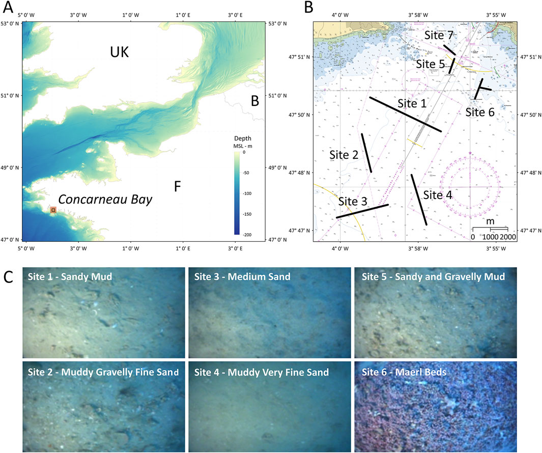
Figure 7. Geographical location; detailed location of Sites 1 to 7; and representative sediment pictures. (A) General location of Concarneau Bay (background: GEBCO_2024 15 arc-second grid); (B) Location of Sites 1 to 7 in Concarneau Bay (background: Service Hydrographique et Océanographique de la Marine, 2016); (C) Visual ground-truthing for Sites I to VI, showing still-frame excerpts from the videos taken on location; for the rock area (Site VII) no picture was taken.

The surveys were conducted using a series of single-beam echosounder units (Kongsberg EK80) working at different frequencies. The EK80 system featured five different transducers covering the full frequency range of current echosounders (excluding low-frequency systems): 38 kHz (actually 35–45 kHz), 70 kHz (50–80 kHz), 120 kHz (95–150 kHz), 200 kHz (170–260 kHz), and 333 kHz (290–440 kHz) transducers (Table 1). Two complete sets of EK80 measurements for Sites 1 and 3 are provided in Supplementary Material - EK80 data and ESAB parameters. All transducers transmitted 256-µs pulse lengths and were operated from the side of the ship, tilted at varying angles controlled by a steering electromechanical device. The EK80 backscatter data collected on the seven sites at 18 different frequencies, and at incident angles varying from normal to 70°, was first interpolated with GSAB into a continuous angular response; each interpolated angular response was then used as an input to the ESAB modelling for every site and frequency. It should be noted that the roughness parameter s₁, theoretically constant for a given seafloor, shows residual frequency dependence (Figure 8D) corresponding to the transducer’s individual properties; this is especially visible at inter-transducer transition frequencies (i.e., near 50, 95, 170, and 290 kHz).

Table 1

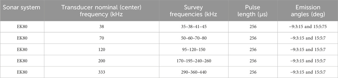
Table 1. Kongsberg EK80 echosounder configuration used during the Concarneau cruise (2023). Five transducers with different nominal center frequencies were employed to cover the full frequency range (35–440 kHz), each operating with multiple discrete survey frequencies. All transducers used 256-µs pulse lengths and were mechanically steered to achieve controlled emission angles ranging from −9° to 75° referenced to the vertical axis.

Figure 8

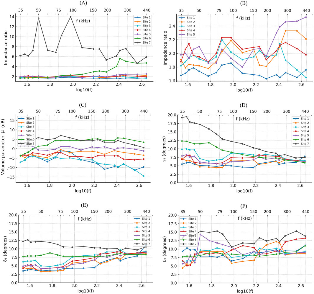
Figure 8. ESAB model parameters as a function of frequency, extracted from datasets recorded on Sites 1 to 7. (A) Impedance ratio (z) all sites; (B) Impedance ratio (z) Sites 1–5; (C) Volume parameter ($\mu$); (D) Roughness Parameter ($s_1$); (E) Facets-slope std. dev. (${\delta }_1$); (F) Facet-slope std. dev. (${\delta }_2$).

The seven sites show an interesting range of acoustic properties, from relatively low impedance on smooth muddy sediments to high-impedance on rough maërl beds and chaotic bedrock. They have been chosen according to the existing knowledge of the seafloor in this region (Ehrhold et al., 2006; Ehrhold et al., 2007). The local sediments were not measured nor analyzed in terms of geotechnical properties; grab samples, as well as video sequences, were taken only for visual identification and description. Hence, the groundtruth available for this dataset is rather qualitative; this is not a serious drawback since the parameters extracted from the ESAB inversion (except the impedance contrast) are not defined to coincide with objective characteristics obtainable by geotechnical measurements.

For each site, the relationships between the ESAB model parameters for 18 frequencies ranging from 35 to 440 kHz and the overall nature of the sediment at each site are discussed qualitatively below. The sediment map of the Bay of Concarneau (Ehrhold et al., 2006) combined with the sediment grabs and video results from the cruise serves as a reference framework for assessing the characteristics of sediments present on the various sites. For the frequency range considered here and for each of the seven sites, Figure 8 shows the evolution of the three parameters (z, μ and $s_1$@150 kHz) plus two distribution parameters (${\delta }_1$ and ${\delta }_2$) obtained from the ESAB model inversion. (see Supplementary Material - EK80 data and ESAB parameters).

3.3 Site 1 – Sandy mud

• Seafloor images show a relatively smooth surface with some bioturbation, which is consistent with the “very fine sandy mud” class previously attributed to this location.

• ESAB inversion results:

◦ The impedance ratio z remains stable across all frequencies at an approximate average of 1.72 (Figures 8A,B). This is the lowest value of all sites, and consistent with fine-grained sediment: compared with classical literature results (Hamilton and Bachman, 1982), the sediment should be classified between Silty Sand and Sand-Silt-Clay.

◦ Volume scattering μ exhibits moderate negative values with an average at −6.7 dB, showing a significant variation from approximately −7.2 dB at 35 kHz to around −9.7 dB at the highest frequencies (Figure 8C).

◦ The roughness parameter $s_1$ at 150 kHz shows consistently low values, averaging 5.6°, with most values around 5.0°–6.0° (Figure 8D), among the lowest values in the dataset.

◦ The facet-slope standard deviation ${\delta }_1$ shows a gradual increase with frequency from approximately 3.5° at 35 kHz to 7.9° at higher frequencies (Figure 8E), consistent with small-scale bioturbation traces becoming more significant at higher frequencies.

◦ The facet-slope standard deviation ${\delta }_2$ remains relatively stable around 9.0° across frequencies (Figure 8F), suggesting consistent larger-scale surficial organization of the sediment.

3.4 Site 2 - Muddy gravelly fine sand

• Seafloor images show a slightly rougher surface compared to Site 1, with the presence of gravel and shell fragments, which is consistent with the “muddy fine sand” previously identified as the dominant sediment type for this site.

• ESAB inversion results:

◦ The impedance ratio z shows a slight variability across frequencies, averaging around 1.99 with a minor increase to about 2.21 at higher frequencies (Figure 8B), suggesting that the acoustic response could become increasingly influenced by the gravel components at higher frequencies.

◦ Volume scattering μ shows moderate negative values with an average of −2.6 dB, ranging from −3.6 dB at low frequencies to a similar value of −3.5 dB at higher frequencies, with intermediate values reaching up to −0.5 dB (Figure 8C). This trend is consistent with mixed sediments exhibiting volume heterogeneities, where gravel components enhance scattering at particular frequencies.

◦ The roughness parameter $s_1$ @150 kHz is slightly higher than Site 1, averaging around 6.0°, with most values between 5.5° and 6.5° (Figure 8D).

◦ ${\delta }_1$ and ${\delta }_2$ show a clear transition with frequency, increasing from about 4.4° at lower frequencies to 8.7° at higher frequencies; however ${\delta }_2$ has an intermediary peak value at 195 kHz (Figure 8E). This suggests a shift in the dominant scattering structure, likely transitioning from mud influence at lower frequencies to gravel components at higher frequencies.

3.5 Site 3 - Medium sand

• The seafloor image displays a uniform texture and appearance, aligning with the medium to fine sand classification previously identified for the area surrounding this site.

• ESAB inversion results:

◦ The impedance ratio z remains stable across all frequencies around a value of approximately 1.95 (Figure 8B), consistent with homogeneous, well-sorted medium sand.

◦ Volume scattering μ exhibits strongly negative values with an average of −7.1 dB, ranging from approximately −4.2 dB to −14.5 dB across the frequency range (Figure 8C). These low values reflect the homogeneous nature of well-sorted medium sand, where fewer internal heterogeneities result in minimal volume scattering.

◦ The roughness parameter $s_1$ @150 kHz shows higher values among sediment sites, averaging around 8.0° with moderate variation, ranging from 6.4° to 10.0° (Figure 8D).

◦ A notable feature is the similarity between the facet-slopes ${\delta }_1$ and ${\delta }_2$ across frequencies (Figures 8E, F). Both parameters range from approximately 6.2°–9.3°. This consistency in roughness parameters aligns with the apparent homogeneity of well-sorted sediments, which produce uniform roughness across scales.

3.6 Site 4 - Muddy very fine sand

• The seafloor image shows a very smooth appearance but with few gravels and bioturbation The area in which this site is included was previously identified as muddy very fine sand.

• ESAB inversion results:

◦ The impedance ratio (z) shows slight variation across all frequencies (Figure 8B), with an average of 2.05, and most values around 2.0–2.1, slightly higher than Sites 1-3 despite its fine grain size, suggesting a significant degree of mud compaction.

◦ Volume scattering μ shows moderate negative values with relatively stable behavior, with an average of −3.8 dB, and values ranging from approximately −3.7 dB to −5.5 dB across all frequencies (Figure 8C). These values suggest relatively homogeneous sediment structure with significant compaction affecting the acoustic response.

◦ The roughness parameter $s_1$ @150 kHz averages around 7.0°, exhibiting slight variation, with most values clustered around 6.5°–7.5°(Figure 8D), higher than Sites 1 and 2.

◦The most striking feature is the strong frequency dependence of the facet-slope std. dev. ${\delta }_2$ with frequency (Figure 8F), showing a clear trend from about 6.6° at 35 kHz to 13.2° at higher frequencies, exhibiting the strongest frequency dependence among sediment sites. In contrast, the facet-slope std. dev. ${\delta }_1$ shows a modest increase from about 4.3° to approximately 8.9° across the frequency range (Figure 8E). This increasing divergence between ${\delta }_1$ and ${\delta }_2$ with frequency suggests a complex surficial sediment texture.

3.7 Site 5 - Sandy and gravelly mud

• Seabed images reveal a more textured surface featuring gravel, shells, and signs of bioturbation. The sediment includes a coarse fraction that complements the very fine muddy sand previously identified in the area encompassing the site.

• ESAB inversion results:

◦ The impedance ratio (z) varies moderately across frequencies, with an average of 2.10, and most values between 1.9 and 2.3 (Figure 8B), reflecting the influence of sand and gravel components.

◦ Volume scattering μ exhibits the highest average of all sediment sites (+0.4 dB), ranging from approximately +1.5 dB at low frequencies to about −1.2 dB at higher frequencies. These high values can be attributed to the combination of low signal attenuation in uncompacted mud, allowing greater penetration, and strong scattering from gravel and sand within the mud matrix.

◦ The roughness parameter $s_1$ at 150 kHz remains relatively consistent across frequencies, averaging around 6.8°, with most values between 6.0° and 7.0° (Figure 8D).

◦ ${\delta }_1$ increases with frequency from 4.9° to 8.9°, and ${\delta }_2$ from 5.7° to 9.0°, but with particularly high values at intermediate frequencies (Figures 8E, F).

3.8 Site 6 - Maërl beds

• Seabed images reveal typical maërl sediments composed of calcareous red algae fragments mixed with shell debris and sand, exhibiting a rough texture and high permeability. The area encompassing Site VI is identified as maërl beds on the sediment map of Concarneau Bay.

• ESAB inversion results:

◦ The impedance ratio z shows a striking increase with frequency, rising from approximately 1.72 at 35 kHz to 4.74 at 440 kHz (Figure 8A), unique among all sites. This suggests that at lower frequencies, acoustic waves interact with the maërl bed as a bulk medium, including water in void spaces, while at higher frequencies, the interaction is increasingly dominated by the individual carbonate fragments.

◦ Volume scattering μ shows a high positive average (+2.8 dB), and consistent increase with frequency with values ranging from −3.8 dB to +5.7 dB (Figure 8C). Given the high impedance contrast at higher frequencies, this likely represents multiple scattering and reverberation within the complex network of carbonate fragments and voids rather than true volume penetration, suggesting a transition in scattering mechanism from bulk-medium behavior at low frequencies to complex surface reverberation at high frequencies.

◦ The roughness parameter $s_1$ at 150 kHz shows a decreasing trend with frequency, starting from 12.3° at 35 kHz and decreasing to about 6.0° at the highest frequencies.

◦ The facet-slope standard deviation shows remarkable consistency, with both ${\delta }_1$ and ${\delta }_2$ maintaining similar values across frequencies (both around 7.7°–10.0°) (Figures 8E,F). This equality between scales suggests that the maërl bed presents similar roughness characteristics regardless of the scale of observation.

3.9 Site 7 – Bedrock

• No seafloor image is available. The area of site 7 is recognized as granitic bedrock in the characterization of benthic habitats of the Concarneau Bay.

• ESAB inversion results:

◦ The impedance ratio z remains consistently high across all frequencies, ranging from approximately 6.19 to 5.93, with intermediate values reaching 14 (Figure 8A), as expected for bedrock. This is especially interesting since, although the fundamental models used in ESAB were not designed for an elastic solid seafloor, the magnitude of these results is acceptable.

◦ Volume scattering μ exhibits high positive values for all frequencies, with an average of 4.1 dB, and values ranging from approximately +3.0 dB at low frequencies to +7.0 dB at mid-frequencies, then decreasing to about +0.6 dB at the highest frequencies (Figure 8C). These values likely reflect multiple reflections within the network of cracks, crevices, and irregular features of the bedrock surface rather than actual internal volume scattering.

◦ The roughness parameter $s_1$ shows the highest values of all sites, decreasing from about 19.5° at low frequencies to approximately 7.3° at higher frequencies (Figure 8D), with an average of 12.7^o. Again, this result is interesting since, while the model is not designed for a high-roughness interface with extreme slopes, the inversion outputs prove to be gross descriptors possibly sufficient for classification.

◦ The facet slope standard deviations ${\delta }_1$ and ${\delta }_2$ remain consistently high across frequencies. ${\delta }_1$ shows a slight decreasing trend from ∼12.5° at low frequencies to ∼10.0° at higher frequencies (Figure 8E) and ${\delta }_2$ remains consistently high, ranging from 13.2° to 13.8°, with peak values at intermediate frequencies (Figure 8F), which may reflect the scale-dependent nature of bedrock roughness.

3.10 Discussion about the model inversion of the Concarneau dataset

The ESAB inversion results across 18 frequencies (35–440 kHz) demonstrate the model’s capability to differentiate seafloor types while maintaining physical consistency across the frequency spectrum. The three-parameter model structure (z, µ, $s_1$ - complemented by two distribution parameters ${\delta }_1$ and ${\delta }_2$) successfully captures distinct acoustic signatures for each site.

The impedance ratio z effectively discriminates between seafloor types. Soft sediments show stable values: sandy mud (Site 1) at 1.73, muddy gravelly fine sand (Site 2) at 1.9–2.1, medium sand (Site 3) at 2.0, muddy very fine sand (Site 4) at 2.1, and sandy gravelly mud (Site 5) at 2.1–2.4. These values are consistent with Hamilton and Bachman’s (1982) classifications, with Site 1 falling between Silty Sand and Sand-Silt-Clay, and Sites 2-5 corresponding to various sand types. The maërl beds (Site 6) exhibit a distinctive frequency-dependent behavior, increasing from 1.7 to 5.6, indicating a transition from bulk-medium response to individual-fragment scattering. Bedrock (Site 7) maintains consistently high values (6–14), clearly distinguishing it from sedimentary substrates.

The volume parameter µ provides additional differentiation between sites and highlights internal inhomogeneity within sediments. Well-sorted sediments such as medium sand (Site 3) show low and stable values (average of −7.1 dB) reflecting minimal internal inhomogeneity. Muddier sediments (Site 1) display slightly higher values (average −6.7 dB), probably due to bioturbation effects. Mixed sediments (sites 2 and 5) show moderately high values (averages −2.6 and 0.4 dB), but variable across frequencies (Site 2: 4.8 to −0.5 dB and Site 5: 1.2 to 1.5 dB), interpretable as due to the presence of gravel or shell components in the sediment matrix. Maërl beds show a high average of 2.8 dB, with values increasing with frequency (from −3.8 to 3.4 dB), likely from multiple scattering among carbonate fragments. Bedrock has the highest average (+4.1 dB) and the highest variation (+0.6 to +7.0 dB) suggesting chaotic interface reverberation to be more likely than true volume scattering; this interpretation requires further validation.

The roughness parameter $s_1$ average across frequencies effectively ranks sites by surface texture: smooth mud (Site 1: 5.6°), mixed sediments (Site 2: 5.9° and Site 5: 6.8°), fine sand (Site 4: 7.0°), medium sand (Site 3: 8.0°), maërl (Site 6: 9.1°), and bedrock (Site 7: 12.6°). Its frequency independence (for sediments Sites 1:5) confirms its physical validity. However, for maërl and bedrock (Sites 6 and 7) the frequency dependency allied to the scale-dependent roughness features becomes apparent.

The facet-slope distribution parameters ${\delta }_1$ and ${\delta }_2$ reveal complex behaviors. Site 1 shows ${\delta }_1$ increasing from 3.5° to 7.9° with frequency (bioturbation effects), while ${\delta }_2$ remains stable (9.3°–10.3°). Site 2 exhibits clear frequency transitions in both parameters (${\delta }_1$: 4.4°–8.7°; ${\delta }_2$: 4.5°–11.0° and then to 8.7), reflecting mud-to-gravel dominance shifts. Site 3 demonstrates a remarkable parameter similarity (${\delta }_1$ ≈ ${\delta }_2$ ≈ 6.3°–9.3°), consistent with homogeneous sediments. Site 4 shows the strongest ${\delta }_2$ frequency dependence (6.6°–13.2°), suggesting complex surface texture. At Site 5, ${\delta }_1$ and ${\delta }_2$ display similar frequency behavior from ∼5.4° at low-frequency to ∼9.0° at high-frequency, indicating well-mixed components. Maërl maintains similar values (${\delta }_1$ ≈8.1° and ${\delta }_2$ ≈ 8.5°) across frequencies, while bedrock shows consistently high values (${\delta }_1$ ≈ 11.0°; ${\delta }_2$ ≈ 13.5°).

Specific questions arise from the increasing impedance of the maërl beds (Site 6) with frequency. At lower frequencies, the acoustic response suggests a bulk-medium behavior where the seabed behaves as a homogenized medium. At higher frequencies, however, individual carbonate fragments are likely to become dominant scatterers. This transition is not well defined and can vary with fragment size, porosity and compaction, making it difficult to establish a clear frequency threshold for the change in scattering mechanism. For instance, the water content analysis would be useful to understand how porosity affects acoustic impedance, particularly at lower frequencies. High-resolution imagery of maërl surfaces could also help to correlate roughness parameters with actual seabed morphology.

For bedrock (Site 7), very high-resolution bathymetry could be used to map fractures and discontinuities, providing a clearer understanding of how these features influence the acoustic response. Comparative analysis with other bedrock types, such as limestone and sandstone, could also shed light on the role of bedrock fracturing in controlling impedance and scattering properties. Addressing these uncertainties through targeted sediment analysis will improve the robustness of ESAB parameters interpretation.

In mixed sediments, such as Sites 2 and 5, the presence of gravel and spatial variation in sediment compaction introduces additional complexity. These factors can contribute to both volume scattering and surface roughness in ways that are difficult to evaluate. To improve the understanding of the relationship between acoustic parameters and seafloor composition, direct sediment characterization should be integrated with acoustic measurements. For soft sediments (Sites 1, 3, 4), porewater content analysis and sediment compaction studies would help to explain impedance variations. Bioturbation assessments using high-resolution imaging or sediment coring could further elucidate the frequency dependence of small-scale roughness. In mixed sediments (Sites 2, 5), more detailed particle size distribution analysis is required to determine the influence of gravel and shell content on acoustic scattering. Sediment profiling and coring could help to detect layering effects, particularly in areas where ${\delta }_2$ shows a strong frequency dependence. In addition, controlled laboratory or in-tank experiments using sediment samples with varying gravel content could improve the interpretation of volume scattering behaviour.

A final point concerns the use of the multi-frequency ESAB model for field data inversion when only one frequency is available, due to sonar limitations or to operational constraints. In practical applications, the ESAB model can effectively operate with single-frequency data, which is typical in many multibeam acoustic surveys that acquire backscatter at multiple incident angles. When multiple sites are insonified at a single frequency, the model can be inverted using the average angular response from each site, enabling site differentiation and classification based on the extracted ESAB parameters. This single-frequency approach (processing an individual vertical data line in Figure 8) provides robust seafloor characterization while maintaining the operational simplicity of conventional survey methods. So, searching for a specific frequency dependence and checking the stability of seafloor properties across the frequency range is then obviously pointless. The ESAB model should then be used anyway, using the default parameters defined and justified above, such as the frequency exponent associated to the roughness spectrum (§2.2.3) or to the volume component (§2.3). The idea is that such assumptions give acceptable results, i.e., as good as can be expected in the context of a single-frequency measurement which is unavoidably bearing a lesser level of information than a multi-frequency dataset.

4 Conclusion

The Extended Seabed Acoustic Backscatter (ESAB) model introduced in this paper proposes a hybrid approach to seafloor characterization based on backscatter angular response, by bridging the gaps between mathematical simplicity (and hence computational efficiency), physical/geoacoustical relevance and finally practical invertibility and interpretability. Starting from the previous GSAB functional model, which was computationally practical and intuitively simple but limited in physical description and lacking the frequency dependence, ESAB was designed on the purpose of addressing these two points with the help of existing backscatter theories duly simplified and adapted. It provides a straightforward and pragmatic modelling of seafloor backscatter as a function of angle, frequency, and seabed properties restricted to a small number of descriptors. It can be used as a predictor for direct computations demonstrating the influence of the various parameters, but its main objective is to be used as an inversion tool for applications to seafloor identification and (to some point) to objective characterization.

As in most classical models, the ESAB model separates seafloor backscatter into two components respectively generated by the rough interface and the inhomogeneous sediment volume. As a gross simplification, the interface (through its impedance and roughness) is the main contributor at steep incidences (typically <20°–30°) while the volume is most often prevalent at more oblique and grazing angles. Interface backscatter may in turn be divided into two components: the small-scale-roughness role is prevalent at the steepest angles, and is relevantly described as a specular effect modelled by the classical facet theory; at oblique incidence, micro-scale roughness generates the Bragg’s scatter regime, described through the small-perturbation approach. Volume backscatter is modelled through a pragmatic geometrical propagation description. For a given seafloor configuration, all these components are assumed to be both angle- and frequency-dependent.

Interface roughness is generally described by a power spectrum, typically expressed as a negative power of spatial frequency describing the interface profile. For a given acoustical frequency, the lower part of the spectrum defines the roughness slopes used in the facets theory; while the upper part of the spectrum gives the roughness elevation variance used in Bragg’s scattering. The transition cut-off between the two parts of the spectrum (or the two regimes) depends on the frequency of the incident acoustic signal and is defined by a condition on the apparent roughness (scaled by wavelength). The facets model is improved beyond its classical formulation by introducing a quantified frequency-dependence of the facets effective size (and hence slope); this is expressed by the condition that the local Rayleigh parameter (ratio of roughness elevation to the signal wavelength) must remain smaller than one for a facet to play its role of plane reflector. Using this condition together with the roughness spectrum expression makes it possible to write the variances of effective roughness slopes and elevations as functions of frequency f and spectrum exponent γ. Finally, the obtained slope variance is proportional to frequency (normalized at an arbitrary value f₀ of 150 kHz corresponding to a reference unit wavelength of 1 cm) powered at an exponent explicitly depending on γ. Similarly, the elevation variance is expressed in f and γ and introduced into the Bragg’s scatter classical expression. A conventional value of γ = 3.333 may be retained for inversion purposes, at least as a starting point.

A further improvement to the classical facet model is the relaxation of the usual hypothesis of a Gaussian distribution of roughness slopes. Since the BS angular response curves near normal incidence may be experimentally observed to exhibit non-Gaussian shapes, the local roughness slope distributions should also be considered non-Gaussian; it is proposed here to model them as a combination of two Gaussian distributions, enabling the fitting of a variety of actual bell-shaped distributions.

The sediment volume component is modelled through a classical approach, featuring the transmission coefficient and the refraction effect at the interface, the absorption coefficient inside the sediment (itself expressed from frequency and local impedance) and a unit-volume parameter with a frequency dependence that is heuristically obtained from the experimental dataset and also normalized at f₀.

The various components of the model (facets, Bragg scatter and volume) are then combined into one resulting BS computation, using connecting terms and limiting the input parameter values in order to improve the numerical stability of the model, especially for purposes of inversion.

Finally, it must be emphasized that the ESAB model is controlled by a simple set of three parameters: the impedance ratio z; the roughness parameter ($s_1$ completed by slope distribution parameters ${\delta }_1$ and ${\delta }_2$) and the volume parameter μ - the two latter being normalized at f₀ = 150 kHz. This is a key point for applicability to future inversion efforts, and it opens the gate to a classification scheme using a simple and intuitive three-dimensional space (impedance/roughness/volume), expecting that the various types of seafloors could show sufficiently different behaviors according to this three-parameter set for providing useful classification results. A number of intermediate quantities are also made available at various steps of the computation (sediment sound speed and attenuation, effective roughness slopes at various frequencies …); however, they are rather indicative values since they are only by-products of the various pragmatic relationships introduced in the model.

Applied in a “direct modelling” approach for predictive computations of backscatter ARCs, ESAB proves to be versatile in effectively producing a wide variety of shapes clearly interpretable according to their input physical parameters. However, its main interest appears in an inversion context for application to field measurement data. The ARC-fitting and parameter inversion process were based here on a simulated annealing algorithm, known to be well-adapted to this category of problems and who proved in this context to be very performant in terms of numerical stability and efficiency, and providing relevant results for the model’s input parameters, corresponding to objective physical properties and potentially usable for practical purposes.

Through the analysis of the Concarneau Bay dataset (seven different seafloor types surveyed with a calibrated echosounder at various angles and frequencies), it was confirmed that the three-parameter model structure (z, μ, $s_1$) provides relevant insights in the physics of seafloor acoustic backscatter while maintaining the efficiency and quality of numerical inversion. For homogeneous sediments, ESAB inversion captures the stable impedance response across frequencies, while for mixed sediments, it can model subtle changes thanks to its frequency-dependent behavior. For the specific acoustic signature of maërl, it proposes a transition from homogenized medium response at low frequencies to individual-scatterer behavior at higher frequencies. Although ill-adapted to a solid substrate like bedrock, ESAB detects the strong impedance contrast that may actually be enough for classification.

The model’s frequency-dependent behavior helps in discriminating between seafloor types, shown by impedance trends across frequencies for different substrates, the estimated evolution of roughness parameters with frequency, and the volume scattering parameter variation with sediment heterogeneity. These results advocate both for the validation of ESAB as a useful tool over a wide range of frequencies (for now covering at least the practical range of echosounders) and for the use of multi-frequency sonar systems for seafloor-mapping surveys, provided that a wide enough range is covered.

Synthesizing several previous approaches ranging from heuristic description to more rigorous physical modelling, ESAB offers a practical tool for seafloor characterization, combining an empirical understanding of the physical backscatter phenomena with adapted (i.e., simplified) theoretical models. Its performance in differentiating, classifying and characterizing seafloor types while maintaining hopefully usable and relevant physical interpretability confirms its value for research and applications in marine acoustic remote sensing. Finally, its functionality across wide range of echosounders frequencies and sediment types is well adapted to the processing of backscatter datasets from modern multibeam sonar systems operated for seafloor mapping applications.

Data availability statement

The raw data supporting the conclusions of this article will be made available by the authors, without undue reservation.

Author contributions

LF: Methodology, Validation, Conceptualization, Software, Writing – original draft, Writing – review and editing. XL: Methodology, Conceptualization, Validation, Writing – review and editing, Writing – original draft. RF: Writing – original draft, Data curation, Methodology, Writing – review and editing, Validation. MR: Writing – original draft, Methodology, Visualization, Validation, Writing – review and editing.

Funding

The author(s) declare that financial support was received for the research and/or publication of this article. This work was partially supported by the MULTISONAR Project, funded by FINEP (Brazilian Innovation Agency) through the Advanced Materials and Strategic Minerals Transversal Action 2020 Program. This work was conducted in the framework of the IFREMER Research and development Project R403 − 006 (Underwater Acoustics). The Belgian Federal Public Service Economy is thanked for taking charge of the article publishing charges (APCs).

Acknowledgments

The authors would like to express their gratitude to Axel Ehrhold (IFREMER) for providing the necessary reports for the sedimentological interpretation of the study areas. We also thank Kongsberg Maritime for making available a special version of their software, allowing the use of the EK80 at different frequencies in CW mode. Finally, we extend our sincere appreciation to the R/V Thalia crew for their dedication and support during the sea measurement campaigns.

Conflict of interest

The authors declare that the research was conducted in the absence of any commercial or financial relationships that could be construed as a potential conflict of interest.

Generative AI statement

The author(s) declare that no Generative AI was used in the creation of this manuscript.

Any alternative text (alt text) provided alongside figures in this article has been generated by Frontiers with the support of artificial intelligence and reasonable efforts have been made to ensure accuracy, including review by the authors wherever possible. If you identify any issues, please contact us.

Publisher’s note

All claims expressed in this article are solely those of the authors and do not necessarily represent those of their affiliated organizations, or those of the publisher, the editors and the reviewers. Any product that may be evaluated in this article, or claim that may be made by its manufacturer, is not guaranteed or endorsed by the publisher.

Supplementary material

The Supplementary Material for this article can be found online at: https://www.frontiersin.org/articles/10.3389/frsen.2025.1619218/full#supplementary-material

Footnotes

¹This is very likely a legacy of the pioneering works on sea-surface roughness modelling: Cox and Munk (1954) successfully fitted a Gaussian slope distribution to their experimental observations.

References

APL-UW (1994). High-Frequency Ocean Environmental Acoustic Models Handbook (APL-UW TR 9407). Seattle, WA. Applied Physics Laboratory, University of Washington.

Google Scholar

Beckmann, P., and Spizzichino, A. (1963). The scattering of electromagnetic waves from rough surfaces. Oxford: Pergamon Press.

Google Scholar

Biot, M. A. (1956a). Theory of propagation of elastic waves in a fluid-saturated porous solid. I. Low-frequency range. J. Acoust. Soc. Am. 28 (2), 168–178. doi:10.1121/1.1908239

CrossRef Full Text | Google Scholar

Biot, M. A. (1956b). Theory of propagation of elastic waves in a fluid-saturated porous solid. II. Higher frequency range. J. Acoust. Soc. Am. 28 (2), 179–191. doi:10.1121/1.1908241

CrossRef Full Text | Google Scholar

Brekhovskikh, L. M., and Lysanov, Y. P. (1982). Fundamentals of ocean acoustics. New York: Springer.

Google Scholar

Buckingham, M. J. (1997). Theory of acoustic attenuation, dispersion, and pulse propagation in unconsolidated granular materials including marine sediments. J. Acoust. Soc. Am. 102 (5), 2579–2596. doi:10.1121/1.420313

CrossRef Full Text | Google Scholar

Caruthers, J. W., and Novarini, J. C. (1993). Modeling bistatic bottom scattering strength including a forward scatter lobe. IEEE J. Ocean. Eng. 18 (2), 100–107. doi:10.1109/48.219530

CrossRef Full Text | Google Scholar

Cox, C. S, and Munk, W. H. (1954). Statistics of the sea surface derived from Sun glitter. J. Mar. Res. 13 (2), 198–227.

Google Scholar

de Moustier, C. (1986). Beyond bathymetry: mapping acoustic backscattering from the deep seafloor with Sea Beam. J. Acoust. Soc. Am. 79, 316–331. doi:10.1121/1.393570

CrossRef Full Text | Google Scholar

de Moustier, C., and Alexandrou, D. (1991). Angular dependence of 12-kHz seafloor acoustic backscatter. J. Acoust. Soc. Am. 90 (1), 522–531. doi:10.1121/1.401278

CrossRef Full Text | Google Scholar

Demer, D. A., Berger, L., Bernasconi, M., Bethke, E., Boswell, K., Chu, D., et al. (2015). Calibration of acoustic instruments. ICES Coop. Res. Rep. No. 326, 133. doi:10.17895/ices.pub.5494

CrossRef Full Text | Google Scholar

Ehrhold, A., Hamon, D., and Guillaumont, B. (2006). The REBENT monitoring network, a spatially integrated, acoustic approach to surveying nearshore macrobenthic habitats: application to the Bay of Concarneau (South Brittany, France). ICES J. Mar. Sci. 63 (9), 1604–1615. doi:10.1016/j.icesjms.2006.06.010

CrossRef Full Text | Google Scholar

Ehrhold, A., Blanchet, A., Hamon, D., Chevalier, C., Gaffet, J. D., and Alix, A. S. (2007). “Réseau de surveillance benthique (REBENT) – Région Bretagne,” in Approche sectorielle subtidale: Identification et caractérisation des habitats benthiques du secteur Concarneau. RST/IFREMER/DYNECO/Ecologie benthique/07-01/REBENT, 78.

Google Scholar

Engman, E. T., and Wang, J. R. (1987). Evaluating roughness models of radar backscatter. IEEE Trans. geoscience remote Sens. (6), 709–713. doi:10.1109/tgrs.1987.289740

CrossRef Full Text | Google Scholar

Fezzani, R., and Berger, L. (2018). Analysis of calibrated seafloor backscatter for habitat classification methodology and case study of 158 spots in the Bay of Biscay and Celtic Sea. Mar. Geophys. Res. 39, 169–181. doi:10.1007/s11001-018-9342-y

CrossRef Full Text | Google Scholar

Fezzani, R., Berger, L., Le Bouffant, N., Fonseca, L., and Lurton, X. (2021). Multispectral and multiangle measurements of acoustic seabed backscatter acquired with a tilted calibrated echosounder. J. Acoust. Soc. Am. 149 (6), 4503–4515. doi:10.1121/10.0005428

PubMed Abstract | CrossRef Full Text | Google Scholar

Fezzani, R., Berger, L., Le Bouffant, N., and Lurton, X. (2025). Multispectral backscatter-based characterization of seafloor sediments using calibrated multibeam and tilted single-beam echosounders. Front. Remote Sens. 6, 1574996. doi:10.3389/frsen.2025.1574996

CrossRef Full Text | Google Scholar

Fonseca, L., and Mayer, L. (2007). Remote estimation of surficial seafloor properties through the application Angular Range Analysis to multibeam sonar data. Mar. Geophys. Res. 28 (2), 119–126. doi:10.1007/s11001-007-9019-4

CrossRef Full Text | Google Scholar

Guillon, L., and Lurton, X. (2001). Backscattering from buried sediment layers: the equivalent input backscattering strength model. J. Acoust. Soc. Am. 109 (1), 122–132. doi:10.1121/1.1329622

CrossRef Full Text | Google Scholar

Hamilton, E. L. (1972). Compressional-wave attenuation in marine sediments. Geophysics 37 (4), 620–646. doi:10.1190/1.1440287

CrossRef Full Text | Google Scholar

Hamilton, E. (1974). “Prediction of deep-sea sediment properties: state-of-the-art,” in Deep-Sea sediments, physical and mechanical properties. Plenum Press, 1–43.

Google Scholar

Hamilton, E. L. (1980). Geoacoustic modeling of the seafloor. J. Acoust. Soc. Am. 68 (5), 1313–1340. doi:10.1121/1.385100

CrossRef Full Text | Google Scholar

Hamilton, E. L., and Bachman, R. T. (1982). Sound velocity and related properties of marine sediments. J. Acoust. Soc. Am. 72 (6), 1891–1904. doi:10.1121/1.388539

CrossRef Full Text | Google Scholar

Ivakin, A. N. (1998). A unified approach to volume and roughness scattering. J. Acoust. Soc. Am. 103 (2), 827–837. doi:10.1121/1.421243

CrossRef Full Text | Google Scholar

Ivakin, A. N. (2004). “Scattering from discrete inclusions in marine sediments,” in Proc. Seventh European Conference on Underwater Acoustics (ECUA 2004), 625–630.

Google Scholar

Ivakin, A. N., and Jackson, D. R. (1998). Effects of shear elasticity on sea bed scattering: numerical examples. J. Acoust. Soc. Am. 103 (1), 346–354. doi:10.1121/1.421094

PubMed Abstract | CrossRef Full Text | Google Scholar

Ivakin, A. N., and Lysanov, Y. P. (1981). Underwater sound scattering by volume inhomogeneities of a bottom medium bounded by a rough surface. Sov. Phys. Acoust. 27 (3), 212–215.

Google Scholar

Jackson, D. R., Winebrenner, D. P., and Ishimaru, A. (1986). Application of the composite roughness model to high-frequency bottom backscattering. J. Acoust. Soc. Am. 79, 1410–1422. doi:10.1121/1.393669

CrossRef Full Text | Google Scholar

Kirkpatrick, S., Gelatt, C. D., and Vecchi, M. P. (1983). Optimization by simulated annealing. Science 220 (4598), 671–680. doi:10.1126/science.220.4598.671

PubMed Abstract | CrossRef Full Text | Google Scholar

Lamarche, G., Lurton, X., Verdier, A. L., and Augustin, J. M. (2011). Quantitative characterisation of seafloor substrate and bedforms using advanced processing of multibeam backscatter - application to Cook Strait, New Zealand. Cont. Shelf Res. 31 (2), S93–S109. doi:10.1016/j.csr.2010.06.001

CrossRef Full Text | Google Scholar

Lurton, X. (2010). An introduction to underwater acoustics – principles and applications. 2nd ed. Berlin: Springer-Verlag.

Google Scholar

Lurton, X., Lamarche, G., Brown, C., Lucieer, V., Rice, G., Schimel, A., et al. (2015). Backscatter measurements by seafloor-mapping sonars. Guidel. Recomm. doi:10.5281/zenodo.10089261200

CrossRef Full Text | Google Scholar

MacKenzie, K. V. (1961). Bottom reverberation for 530- and 1030-cps sound in deep water. J. Acoust. Soc. Am. 33, 1498–1504. doi:10.1121/1.1908482

CrossRef Full Text | Google Scholar

McKinney, C. M., and Anderson, C. D. (1964). Measurements of backscattering of sound from the ocean bottom. J. Acoust. Soc. Am. 36 (1), 158–163. doi:10.1121/1.1918927

CrossRef Full Text | Google Scholar

Metropolis, N., Rosenbluth, A. W., Rosenbluth, M. N., Teller, A. H., and Teller, E. (1953). Equation of state calculations by fast computing machines. J. Chem. Phys. 21 (6), 1087–1092. doi:10.1063/1.1699114

CrossRef Full Text | Google Scholar

Montereale Gavazzi, G. O. A. (2019). Development of seafloor mapping strategies supporting integrated marine management: application of seafloor backscatter by multibeam echosounders. Ghent, Belgium: Ghent University. PhD Thesis.

Google Scholar

Mourad, P. D., and Jackson, D. R. (1989). “High frequency sonar equation models for bottom backscatter and forward loss,” in Proceeding of Oceans'89 (Marine Technology Society and IEEE), Seattle, WA, USA, 18-21 September 1989 (IEEE), 1168–1175.

CrossRef Full Text | Google Scholar

Novarini, J. C., and Caruthers, J. W. (1994). The partition wavenumber in acoustic backscattering from a two-scale rough surface described by a power-law spectrum. IEEE J. Ocean. Eng. 19 (2), 200–207. doi:10.1109/48.286642

CrossRef Full Text | Google Scholar

Novarini, J. C., and Caruthers, J. W. (1998). A simplified approach to backscattering from a rough seafloor with sediment inhomogeneities. IEEE J. Ocean. Eng. 23 (3), 157–166. doi:10.1109/48.701188

CrossRef Full Text | Google Scholar

Rice, S. O. (1951). Reflection of electromagnetic waves from slightly rough surfaces. Commun. Pure Appl. Math. 4 (2), 351–378. doi:10.1002/cpa.3160040206

CrossRef Full Text | Google Scholar

Service Hydrographique et Océanographique de la Marine (2016). De Loctudy à Concarneau.

Google Scholar

Shaw, P. R., and Smith, D. K. (1990). Robust description of statistically heterogeneous seafloor topography through its slope distribution. J. Geophys. Res. 95 (B6), 8705–8722. doi:10.1029/jb095ib06p08705

CrossRef Full Text | Google Scholar

Stockhausen, J. H. (1963). Scattering from the volume of an inhomogeneous half-space. Dartmouth, N. S.: Naval Research Establishment. Report No. 63/9.

Google Scholar

Stoll, R. D. (1989). Sediment acoustics (lecture notes in earth science). Berlin: Springer-Verlag.

Google Scholar

Thorsos, E. I., and Jackson, D. R. (1989). The validity of the perturbation approximation for rough surface scattering using a Gaussian roughness spectrum. J. Acoust. Soc. Am. 86 (1), 261–277. doi:10.1121/1.398342

CrossRef Full Text | Google Scholar

Valenzuela, G. R. (1978). Theories for the interaction of electromagnetic and oceanic waves: a review. Boundary-Layer Meteorol. 13, 61–85. doi:10.1007/bf00913863

CrossRef Full Text | Google Scholar

Wong, H. K., and Chesterman, W. D. (1968). Bottom backscattering near grazing incidence in shallow water. J. Acoust. Soc. Am. 44, 1713–1718. doi:10.1121/1.1911318

CrossRef Full Text | Google Scholar

Yang, Y., He, G. W., Ma, J. F., Yu, Z. Z., Yao, H. Q., Deng, X. G., et al. (2020). Acoustic quantitative analysis of ferromanganese nodules and cobalt-rich crusts distribution areas using EM122 multibeam backscatter data from deep-sea basin to seamount in Western Pacific Ocean. Deep Sea Res. Part I Oceanogr. Res. Pap. 161, 103281. doi:10.1016/j.dsr.2020.103281

CrossRef Full Text | Google Scholar