Validation of DSCOVR-EPIC total column O3 retrievals using ground-based Pandora as well as OMPS, OMI, and TEMPO satellite data

The Earth polychromatic imaging camera (EPIC) onboard the deep space climate observatory (DSCOVR) began obtaining fully illuminated Earth images across 10 wavelength bands on 6 July 2015. The ultraviolet bands 317, 325, 340, and 388 nm are used to retrieve the total column ozone (TCO) values at different local times during the day. On 28 June 2019, the spacecraft experienced a gyroscope failure; after recovery, the EPIC TCO values retrieved from 2021 to 2024 still agree well with those obtained from the ground-based Pandora spectrometer instruments in terms of both the hourly and weekly average basis. The hourly EPIC TCO values show more variability than the matched Pandora TCO values but generally deviate within 2% while tracking the shape of the Pandora daily variations in most cases. At 13:30 hours, the TCO data from the ozone and mapping profiler suite (OMPS) and ozone monitoring instrument (OMI) are also observed to frequently agree with the time-matched Pandora and EPIC TCO values. In addition, comparisons were made with the version-3 (V03) hourly TCO retrievals from the US tropospheric monitoring of pollution (TEMPO) geostationary satellite over two North American sites, namely, Toronto (Canada) and Dearborn (Michigan, United States). The long-term weekly lowess average EPIC and Pandora TCO values agree with deviations of less than 2%, as does the 3-week lowess average of the OMPS TCO value. An analysis of the TCO values from Pandora and 1 year of TEMPO V03 suggests that the noon TCO values are 2%–5% higher than the morning and afternoon values.

1 Introduction

The Earth polychromatic imaging camera onboard the deep space climate observatory (DSCOVR-EPIC) is a satellite instrument launched on 11 February 2015 and is in orbit around the Earth–Sun gravitational balance Lagrange point L₁. Starting on 6 July 2015, the EPIC obtained nearly fully illuminated Earth images using 10 narrowband filters on two filter wheels in front of a 2048 × 2048 pixel hafnium-coated charged coupled device (CCD) detector in the wavelength range of 317–780 nm (Herman et al., 2018; Marshak et al., 2018); this window spans ultraviolet (UV, 317–388 nm), visible (443–688 nm), and near-infrared (NIR, 764–780 nm) wavelengths. The Earth-viewing exposure times were determined to produce CCD well filling to 80% for most bright scenes with high clouds. The optical transmission and radiometric sensitivity of the CCD have been almost constant since the first data obtained in June 2015, allowing the exposure times to be constant during the current life of the mission (2015–2025). The UV filters were selected such that the ozone amounts, cloud reflectivity, and aerosol properties could be derived from the observations. The remaining filters provide additional aerosol properties, vegetation and sunlit leaf area indices, volcanic activity, as well as cloud and aerosol heights (using the oxygen A and B band filters). The UV channels 317.5, 325, 340, and 388 nm were used to retrieve the total column ozone version-3 (TCO V03) values approximately once per hour during the northern hemisphere (NH) summer and approximately once every 90 min during the NH winter. The result for any given location on the rotating (15° per hour) illuminated Earth entails retrieval of 4–10 data points per day at different local solar times when the solar zenith angle (SZA) is less than 70°.

The ozone retrieval algorithm was originally described in Herman et al. (2018). Since then, there have been significant improvements in the geolocation of the retrieved pixels, allowing improved radiance ratios of the sequentially observed filter wavelengths needed for the retrieval algorithm. There also have been improvements in the CCD flat field, which refers to the ratio of the sensitivity of one pixel relative to the other pixels, as well as correction for stray light from the telescope optics and support structures. At present, the ozone retrievals are mature and stable and can be usefully compared with accurate ground-based retrievals from the worldwide Pandora spectrometer network (https://www.pandonia-global-network.org/); this network currently comprises approximately 150 instruments that each obtain TCO measurements once every 2–4 min. The Pandora ozone retrievals are derived using spectral fitting in the range of 305–330 nm along with reflectivity corrections at 388 nm and have been successfully compared with measurements from the Brewer spectrometer, Dobson, and ozone monitoring instruments (Herman et al., 2015; Tzortziou et al., 2012; Baek et al., 2017). Useful comparisons can also be made with satellite instruments like the validated ozone monitoring instrument (OMI) onboard the polar-orbiting AURA satellite (McPeters et al., 2008; Bak et al., 2015) and polar-orbiting ozone mapping and profiler suite nadir mapper (OMPS-NM) onboard the Suomi national polar-orbiting partnership (SNPP) satellite (Flynn et al., 2014) as well as with samples over the Pandora sites from the first year of the preliminary TCO V03 data from the US tropospheric monitoring of pollution (TEMPO) geostationary satellite that has obtained measurements over North America once per hour local solar time since September 2023. All satellite retrievals of ozone values use the total ozone mapping spectrometer (TOMS)-type wavelength ratio method based on radiative transfer (TOMrad) look-up tables. Pandora uses spectral fitting based on convolution of the ozone absorption cross section with the solar irradiance at ground. The TOMS ozone retrieval algorithm estimates the TCO from backscattered UV radiances at three wavelengths (McPeters and Labow, 1996; McPeters et al., 2008; Herman et al., 2018).

The 25 Pandora instruments used in the present study are listed in Table 1. All these instruments are single-spectrometer versions in the spectral range of 290–550 nm with a spectral resolution of 0.6 nm. The EPIC instrument has no onboard means of in-flight calibration; hence, radiometric calibrations are performed via vicarious comparisons of geographically and temporally matched scenes in the equatorial region with well-calibrated low Earth orbit (LEO) satellites, i.e., SNPP OMPS-NM for the UV channels and moderate resolution imaging spectroradiometer (MODIS) for the visible and NIR channels (Herman et al., 2018; Marshak et al., 2018). Common scenes from the equatorial and near-equatorial regions are used to closely match the SZAs and view zenith angles (VZAs) observed by both the EPIC and LEO satellites. The present work shows the degrees of agreement among five instruments, namely. EPIC, Pandora, TEMPO, OMPS, and OMI, for the TCO over selected Pandora sites in terms of both daily variations and weekly averages for the years 2015–2024, where available. There is a 9-month data gap for the period from June 2019 to March 2020 because of failure of the pointing gyroscopes that were later replaced with the onboard star tracker and revised flight software.

Table 1

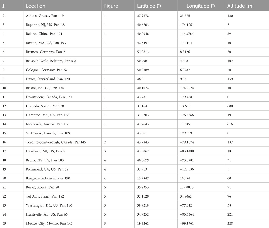
Table 1. Pandora sites in order of first appearance.

2 Comparisons with EPIC ozone data

Figure 1 shows a comparison of the EPIC overpass TCO data retrievals for 16 Pandora sites at local solar times compared to Pandora TCO values at the same Greenwich mean times (GMTs). The retrieval days were selected such that the Pandora had nearly continuous data during the day, suggesting that these days were relatively clear of cloud cover. The EPIC TCO retrievals at high SZAs (early mornings and late afternoons) are not accurate because of spherical geometry errors in the retrieval algorithm; further, the Pandora data show similar but smaller effects. The EPIC TCO standard deviations (1-σ, blue stars) are shown in Figures 1–3; further, the TEMPO standard deviations are similar to those of the EPIC data, while the variances of the Pandora data are small but obvious from examination of successive data points.

Figure 1

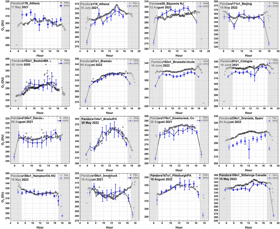
Figure 1. Comparison of the Earth polychromatic imaging camera (EPIC) total column ozone (TCO) overpass data (blue stars) for 16 Pandora sites at the local solar times (07:00 to 17:00) with Pandora TCO values (small open circles) at the same Greenwich mean time (GMT). The retrieval sites were selected from Europe, United States, China, and Canada. The gray areas indicate large solar zenith angles (SZAs) >75° where the retrievals may not be valid.

Figure 2

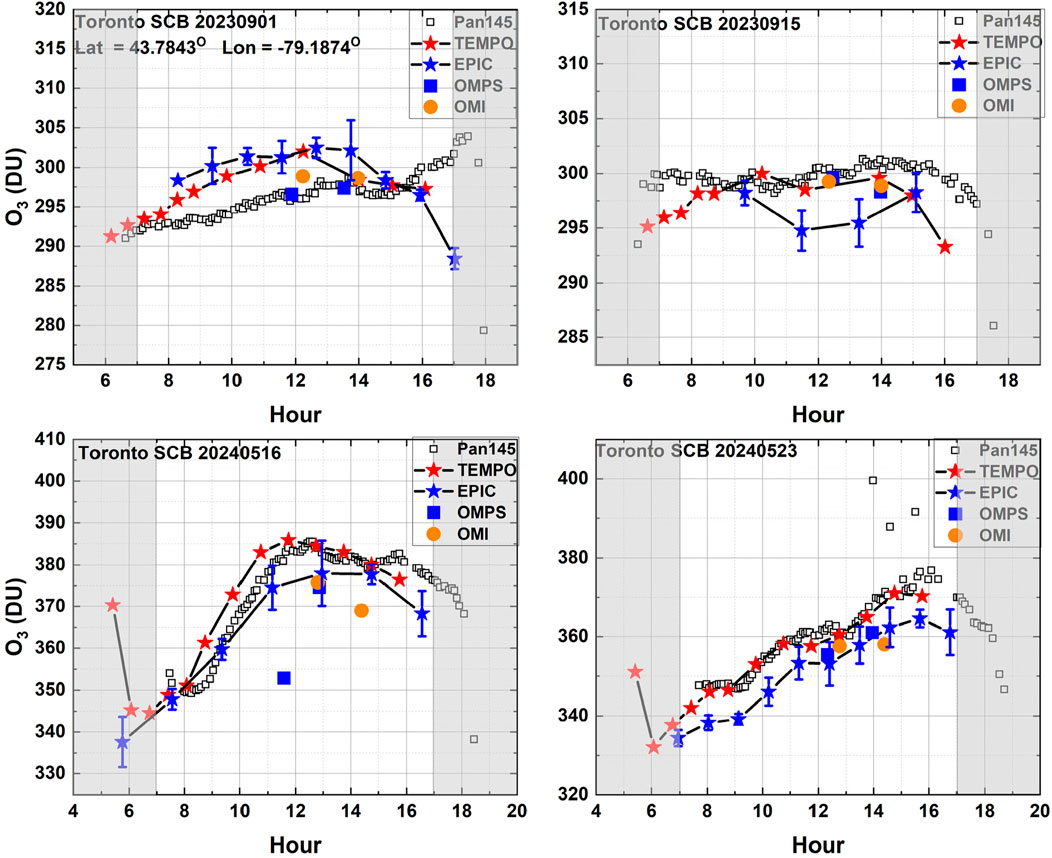
Figure 2. Four different days (1 and 15 September 2023, 16 and 23 May 2024) of EPIC ozone retrievals over the Pandora 145 site (small open squares) at Toronto-Scarborough, Canada (latitude = 43.7843°, longitude = −79.1874°, and altitude = 137 m) vs. local solar time in hours. The red stars are the tropospheric monitoring of pollution (TEMPO) overpass TCO values, and the blue stars are the EPIC overpass TCO values at the same GMTs as the Pandora data. The orange circles are the ozone monitoring instrument (OMI) TCO values, while the blue squares are the ozone mapping and profiler suite (OMPS) TCO values. The gray areas indicate large SZAs >75° where the retrievals may not be valid.

Figure 3

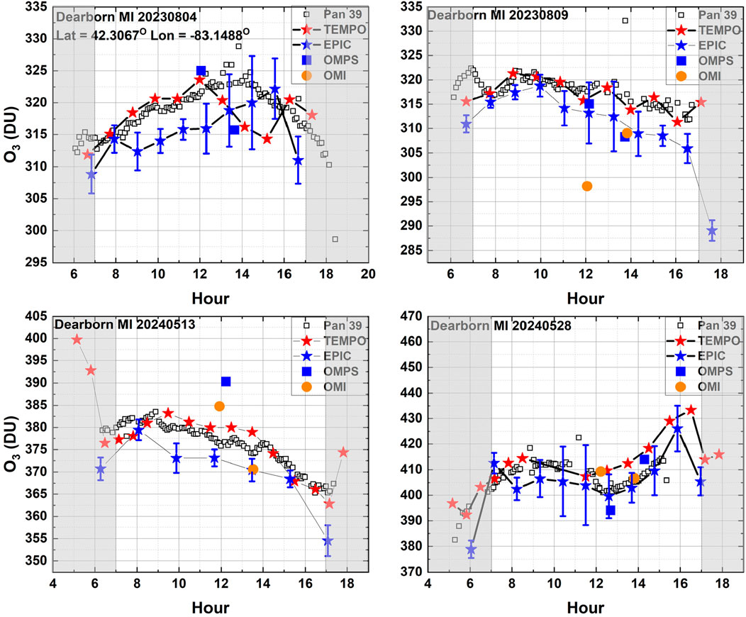
Figure 3. Similar to (Figure 2) Four different days (4 and 9 August 2023, 13 and 28 May 2024) of EPIC ozone retrievals over the Pandora 39 site (open squares) at Dearborn, Michigan, United States (latitude = 42.3067°, longitude = −83.1488°, and altitude = 137 m) vs. local solar time in hours. The red stars are the TEMPO overpass TCO values, and the blue stars are the EPIC overpass TCO values at the same GMTs as the Pandora data. The orange circles are the OMI TCO values, while the blue squares are the OMPS TCO values. The gray areas indicate large SZAs >75° where the retrievals may not be valid.

For most Pandora sites, the data agree within 2% (approximately 6 Dobson unit (DU)) throughout the day, except at high SZAs. The EPIC data track the shapes of the diurnal TCO variations observed by Pandora. Exceptions to these are the near-noon values for Granada (Spain) and St. George (Canada) as well as the near-11:00 values at Downsville (Canada). In mountain areas like Innsbruck in Austria, the ozone layer can vary geographically over short distances because of atmospheric pressure waves. This means that Pandora, which makes local observations, may be observing different TCO amounts than those of the EPIC gridded satellite data that are averaged over 0.25° × 0.25° grids or approximately over a field of view of 25 × 25 km². Figure 2 shows a comparison of the observed TCO values over Toronto (Canada) for four different days, i.e., two in September and two in May. The comparisons shown are for the Pandora, TEMPO, EPIC, OMPS, and OMI data. The retrieval error estimates for EPIC are given in Figures 1–3, and similar error estimates apply for the TEMPO retrievals; the error estimates for Pandora are much smaller as each point is the average of many individual measurements.

Comparison of the Toronto data shows a problem with frequent cloud cover that is obvious when there are missing or noisy Pandora data. After screening for the Pandora data quality, the agreement between EPIC and Pandora 145 are noted to be quite good. It also appears that the EPIC TCO values are systematically lower than the Pandora TCO values most of the time (see also Figure 3 for Dearborn, Michigan, United States). EPIC tracks the Dearborn Pandora 39 fairly well (within 5 DU) as a function of the time of day. On 14 July 2023, Pandora 39 lost its ability to retrieve TCO data from 12:00 to 15:00 probably because of the presence of clouds between Pandora and the Sun. A test run of the TEMPO V03 geostationary satellite data is seen to have good agreement with Pandora (Figures 2, 3).

Another way of looking at the data comparisons (Figures 4, 5) is in terms of 3-week running TCO averages over the 3.5-year period from 2021 to 2024. The 3-week running average is based on the lowess(f) procedure (Cleveland, 1979; Cleveland et al., 1988), where f is the fraction of the time series. The lowess function reduces the weight of outliers in a manner similar to that of the linear least-squares fit to the data. All the Pandora and EPIC data are included regardless of the SZAs. The small systematic differences between the EPIC and Pandora TCO values persist in the weekly averages but are less than 2%. In some cases like that of Pandora 20 in Busan (Korea), there are missing data as well as obvious errors during late 2023 to 2024. For two sites at Dearborn and Hampton (Virginia, United States), the Pandora data are missing in 2021. A 3-week lowess average of the OMPS TCO values (solid magenta line) has been added for comparison in these two figures; the agreement between the averages is better than 2%, except for Busan where there is a clear error in the Pandora 20 TCO values after August 2023. At most sites, the agreement among the TCO values of the three satellites and ground-based Pandora are very close for the 3–4 years of comparison; an exception to this is Busan, where Pandora 20 appears to have a sun-tracker pointing issue after October 2023.

Figure 4

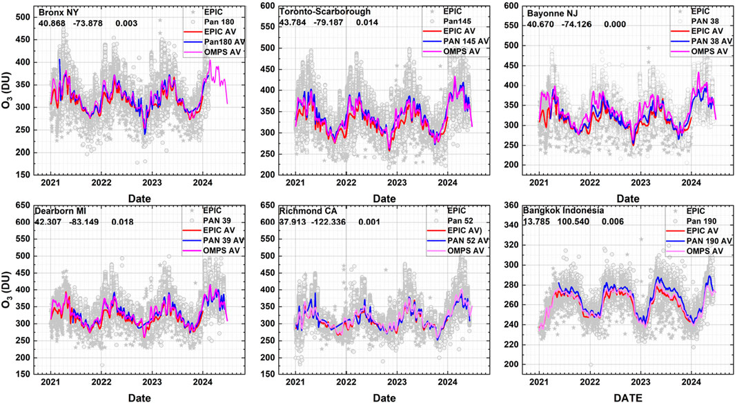
Figure 4. Solid lines depicting the 3-week TCO averages from six Pandora sites using the lowess (3-week) procedure. The names, Pandora numbers, latitudes, longitudes, and altitudes of each of the Pandora sites are given in the figure. The stars and red line are the EPIC TCO values, while the open circles and blue line are the Pandora TCO values. The magenta line represents the 3-week average OMPS TCO value.

Figure 5

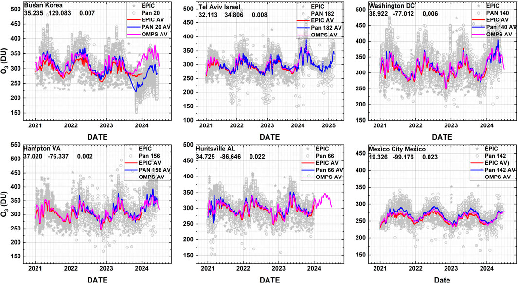
Figure 5. Solid lines depicting the 3-week TCO averages from six Pandora sites using the lowess (3-week) procedure. The names, Pandora numbers, latitudes, longitudes, and altitudes of each of the Pandora sites are given in the figure. The stars and red line are the EPIC TCO values, while the open circles and blue line are the Pandora TCO values. The magenta line represents the 3-week average OMPS TCO value.

3 Comparison of EPIC TCO values with OMI and OMPS data

A closer examination of Figures 4, 5 suggests that EPIC has a systematic offset with respect to the OMI and OMPS data. The EPIC TCO records from May 2015 to 2025 (present) can be compared with similar records from the OMI and OMPS to estimate the bias between these satellite records. Figure 6 shows the individual time-series data from the EPIC and OMI for four sites, namely, Beltsville (Maryland, United States), Athens (Greece), Dearborn, and Richmond (California, United States), that are typical for mid-latitude NH sites. The OMPS TCO values have been omitted from Figure 6 since they are closely matched with the OMI data, as shown in Figure 7 for the percentage differences.

Figure 6

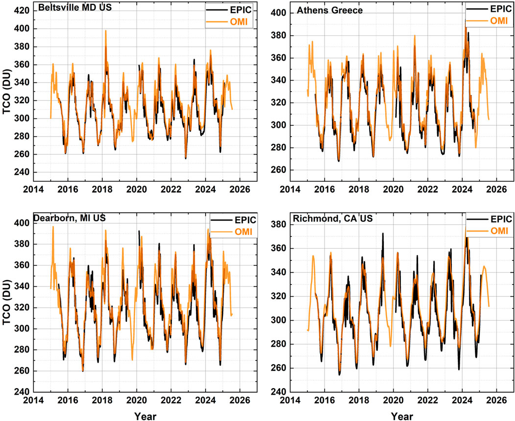
Figure 6. Time-series data comparisons between EPIC and OMI TCO values at four locations.

Figure 7

Figure 7. Percentage differences in TCO values among EPIC, OMI, and OMPS data at four sites in the northern hemisphere. The 10-year average values of the percentage differences are given for OMI–EPIC (<A>), OMPS–EPIC (<B>), and OMI–OMPS (<C>).

To compare the time-series data for small differences, they must be examined on a common time scale by interpolation with adequate resolution to reproduce the main features of each time series. To estimate the long-term percentage differences, approximately 1,000 points are sufficient in each series. Next, the percentage differences were calculated for OMI vs. EPIC, OMPS vs. EPIC, and OMI vs. OMPS data. Finally, the percentage differences were smoothed using lowess(0.05) to remove small fluctuations and are shown in Figure 7 (NH), Figure 8 (equatorial region (ER)), and Figure 9 (southern hemisphere (SH)). The symbols A, B, and C are the long-term percentage differences in the time series, while <A>, <B>, and <C> represent the 10-year average values. In the NH and SH, there are long-term systematic biases of 2%–3% (approximately 6–9 DU), with the EPIC TCO values being less than both the OMI and OMPS data. The long-term OMI and OMPS TCO values differ by less than 1%, and the average differences are indicated in the graphs. However, in the ER, the OMPS and OMI data disagree by approximately 1.5%, with OMI > OMPS TCO values.

Figure 8

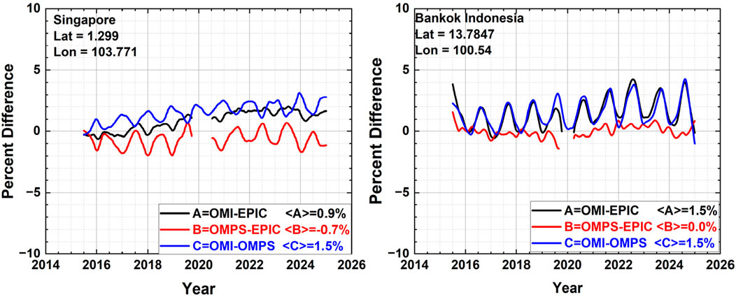
Figure 8. Percentage differences in TCO values among EPIC, OMI, and OMPS data at two sites in the equatorial region. The 10-year average values of the percentage differences are given for OMI–EPIC (<A>), OMPS–EPIC (<B>), and OMI-OMPS (<C>).

Figure 9

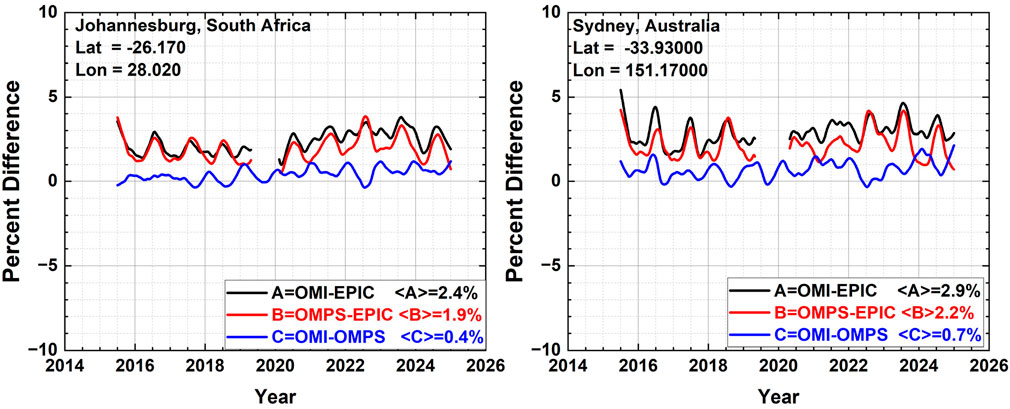
Figure 9. Percentage differences in TCO values among EPIC, OMI, and OMPS data at two sites in the southern hemisphere. The 10-year average values of the percentage differences are given for OMI–EPIC (<A>), OMPS–EPIC (<B>), and OMI–OMPS (<C>).

4 Systematic diurnal variations of the TCO

Accurate measurements of the TCO at different times of the day with the DSCOVR-EPIC and TEMPO satellite instruments or with ground-based instruments like Pandora can provide answers to whether there are significant long-term systematic differences in the ozone levels in the morning or afternoon than the noon. In Figures 1–3, significant diurnal variations can be observed for most days. Based on model studies and known chemical time constants, there should be only small diurnal variations (a few percent) of the TCO values (Schanz et al., 2021) from the troposphere and upper stratosphere in the absence of weather and atmospheric wave effects. Model studies (Strode et al., 2019) also suggest that the tropospheric ozone peaks in the afternoon, whereas the stratospheric ozone amounts vary only seasonally and inversely as a function of the noontime SZAs. Figures 10, 11 show the stepwise method used to estimate the possible systematic diurnal variations at two locations, namely, Beltsville and Edwards (California, United States), respectively. For EPIC, the following analyses in Figures 10, 11 show that the TCO data indicate systematic variations; in these figures, panels a, b, and c show the original data in three periods of 9:00 to 10:00, 11:30 to 12:30, and 14:00 to 15:00, respectively, along with their lowess (3-week) fits. The EPIC sampling (1 h in the summer and 2 h in the winter) of the diurnal variations may not be sufficient to show the significant systematic effects.

Figure 10

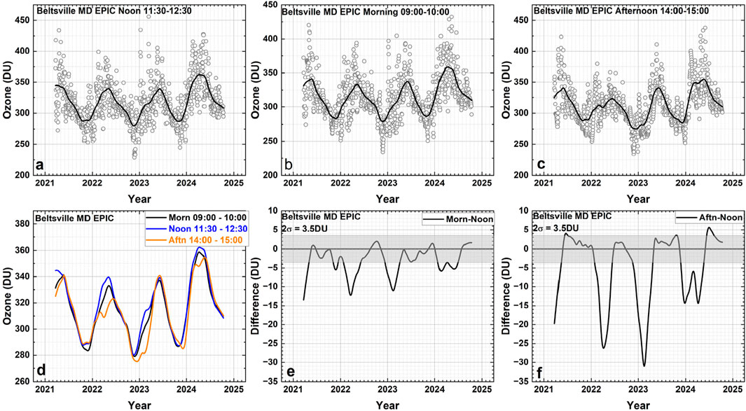
Figure 10. TCO(t) values from EPIC at Beltsville (Maryland, United States) shown as small open circles: (a) morning 9:00 to 10:00, (b) noon from 11:30 to 12:30, and (c) afternoon 14:00 to 15:00. (d) Lowess(0.0088) 3-weekly averages from (a–c) plotted together, along with lowess plots for (e) morning–noon and (f) afternoon–noon differences. The gray areas in (e, f) represent ±2σ, where σ is the standard error.

Figure 11

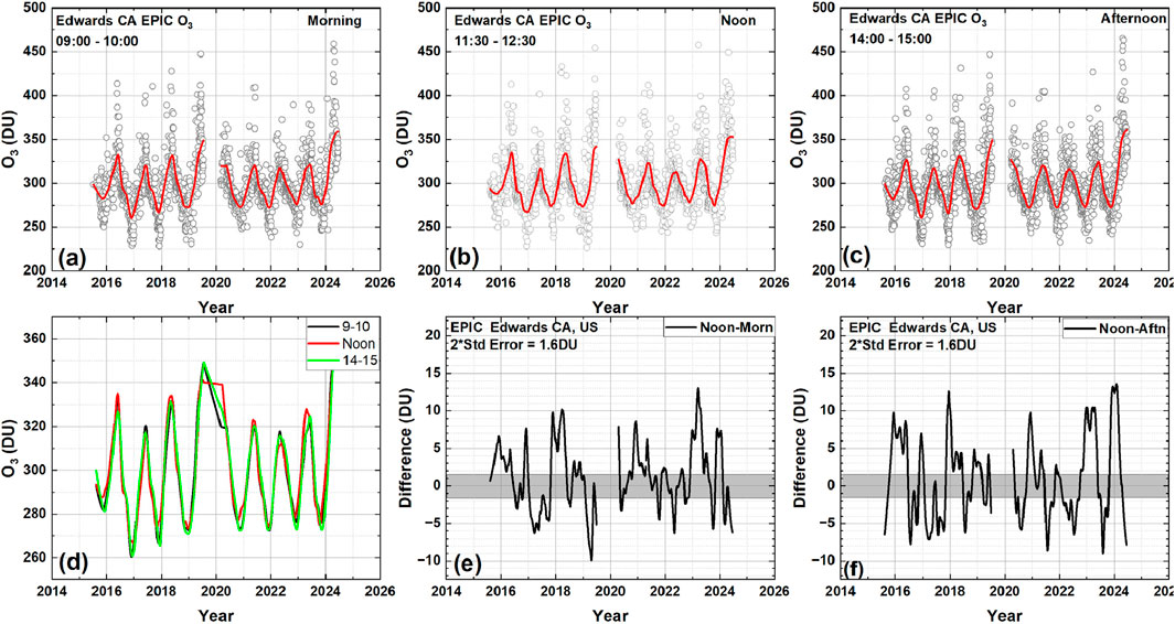
Figure 11. TCO(t) values from EPIC at Edwards Air Force Base (California, United States) shown as small open circles: (a) morning 9:00 to 10:00, (b) noon from 11:30 to 12:30, and (c) afternoon 14:00 to 15:00. (d) Lowess(0.0088) 3-weekly averages from (a–c) plotted together, along with lowess plots for (e) morning–noon and (f) afternoon–noon differences. The gray areas in (e, f) represent ±2σ, where σ is the standard error.

Panel d in Figure 10 shows that the 3-week averages are similar in value; the differences are shown in panels e and f, where the afternoon differences are ±6DU or ±2% and the morning differences are ±4DU or ±1%. Twice the standard error of the mean is 2σ or ±3.5 DU, so that most of the variations are not statistically significant. Panel e suggests that the noon TCO is systematically more than in the morning during winters. Panel f suggests that there may be more TCO at noon than in the afternoon during winter. However, the winter sampling interval of the diurnal variations is 2 h, which may not be sufficient to guarantee these conclusions. In Figure 11, the small differences shown in panels e and f are mostly less than ±10DU or ±3%; here, twice the standard error of the mean is 2σ or ±1.5 DU, so that most of the variations are statistically significant. However, the pattern from one year to the next is random, indicating that EPIC does not detect systematic diurnal variations over Edwards. Similar EPIC results are seen at the other locations.

The diurnal variations of TCO as seen by the geostationary satellite TEMPO over six specified locations in the United States and Canada are shown in Figure 12. The TEMPO TCO values show small systematic differences depending on the observed locations. The TCO over Bronx (New York, United States) is less in the afternoon than noon by approximately 5 DU, while Toronto appears to have morning TCO values less than those at noon; the afternoon TCO values are lower than the noon values at Richmond, while Huntsville (Alabama, United States) shows maximum TCO at noon; Bayonne (New Jersey, United States) has lower afternoon TCO values than noon, while Dearborn has lower morning TCO values than noon. The differences with the values at noon are of the order of 5 DU (<2% of TCO) and may be attributed to tropospheric ozone changes.

Figure 12

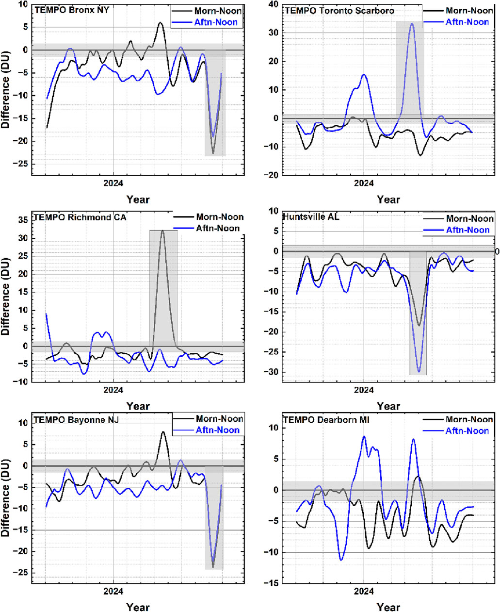
Figure 12. Diurnal TCO variations of TEMPO V03 with 2σ = ±1.5 DU. The vertical gray bars are centered around the ozone retrieval errors. The calculations here are similar to those in Figures 8, 9. The smooth lines are lowess (0.1) or averaged approximately 1 month at morning (09:00 to 10:00), noon (11:30 to 12:30), and afternoon (14:00 to 15:00). The horizontal gray areas are the estimated 2σ standard errors of the mean for the time series, while the vertical gray areas mark possible retrieval errors in the original TCO time series.

The ground-based Pandora spectrometers have the best time sampling of at least one recorded measurement every 2 min that clearly tracks the TCO diurnal variations. Figure 13 shows the estimates of the systematic diurnal variations at the same six sites as in Figure 12. Except for Bayonne, whose values disagree with TEMPO data, the TCO is greater at noon (11:30 to 12:30) than morning (09:00 to 10:00) or afternoon (14:00 to 15:00) by 1%–3%. The TEMPO data show that the TCO values at all six sites are greater at noon (11:30 to 12:30) than morning (09:00 to 10:00) or afternoon (14:00 to 15:00) by 3 DU or approximately 1%. Detailed agreements are not expected since the spatial sampling between the satellites is different, with 18 × 18 km² for EPIC and 2 × 4.75 km² for TEMPO at nadir. Pandora views areas of 0.2 × 0.2 km² at an altitude of 25 km, but the views in different directions track the solar position in the sky. EPIC samples at the rate of once per hour from May to August and once every 2 h from August to April, while TEMPO samples once per hour. The TEMPO and Pandora TCO data suggest that there are systematic long-term differences between the morning and afternoon TCO values compared to near-noon values at least at some sites and that these differences are not caused by random weather patterns. The long-term differences with near-noon TCO values are small (of the order of a few DU) enough to be considered local tropospheric variations.

Figure 13

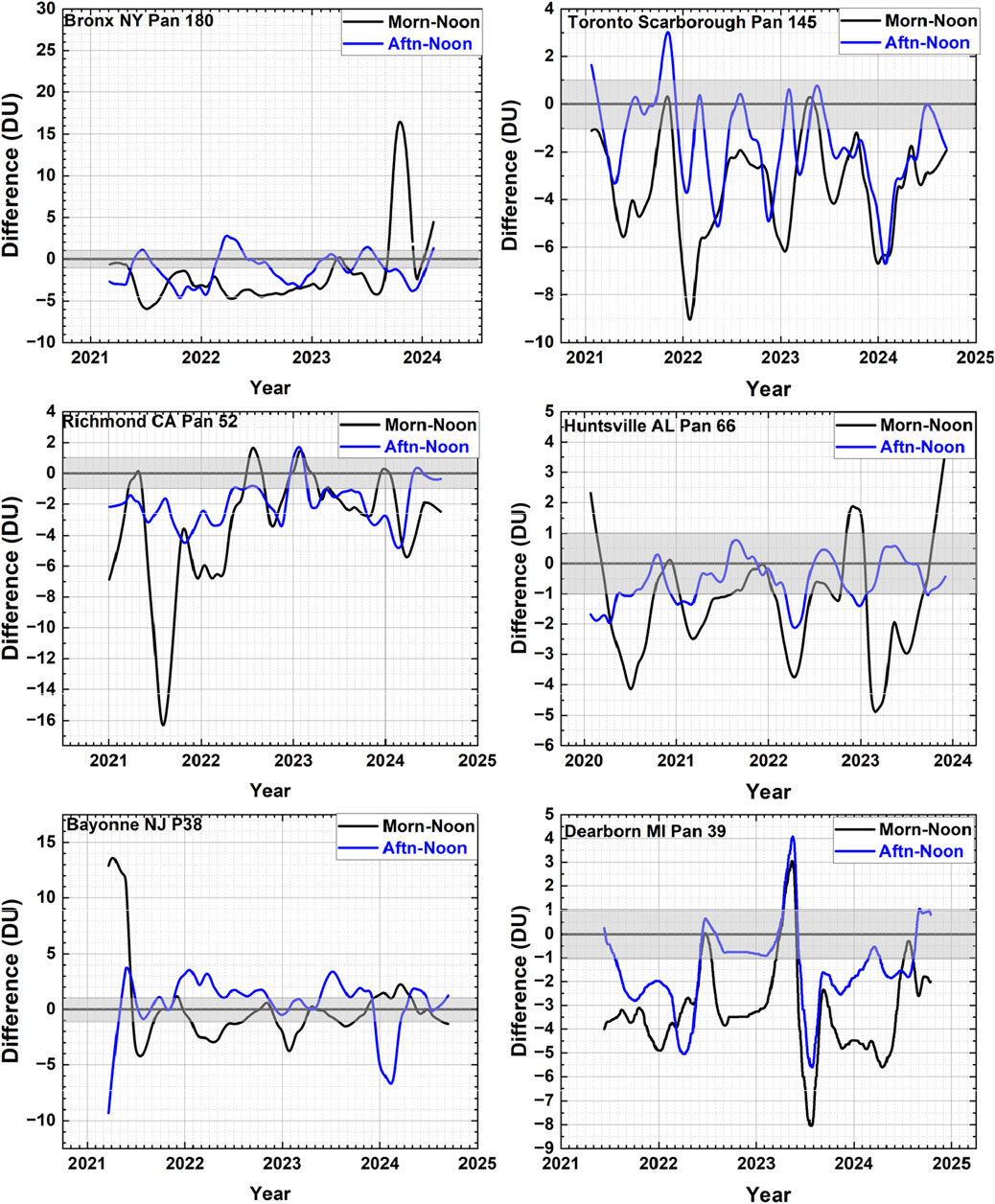
Figure 13. Diurnal TCO variations of the Pandora ground-based instruments with 2σ = ±1 DU. The calculations here are similar to those in Figures 8, 9. The smooth lines are lowess(0.1) or averaged approximately 1 month at morning (09:00 to 10:00), noon (11:30 to 12:30), and afternoon (14:00 to 15:00).

5 Summary

The hourly retrievals of TCO by EPIC over most Pandora sites differ by less than 5 DU (1%–2%) from the values retrieved using the Pandora instruments, as shown in Figures 1–3, and from the TEMPO TCO retrievals, as shown in Figures 2, 3. There are some comparisons that differ by larger amounts (e.g., 10 DU over Grenada, Figure 1). Other sites for which data are not shown have similar TCO values for EPIC and Pandora that are within 2% of each other. The near-noon OMI and OMPS data comparisons also show differences of mostly 1%–2%, with occasional larger differences. Weekly averages for the period from 2021 to 2023 in terms of the lowess fits of the retrieved TCO values show close agreement between EPIC and Pandora as well as and the 3-week lowess averages of the OMPS TCO values. Comparisons of the long-term percentage differences from May 2015 to May 2025 among the EPIC, OMI, and OMPS data show systematic biases of 2%–3% in the NH and SH, with the EPIC TCO being less than the corresponding OMI and OMPS values. In the ER, the OMI TCO is greater than the OMPS TCO by1.5%, while the EPIC TCO is close to that of the OMPS; here, the differences are small but systematic. Agreement within 2% suggests that the EPIC UV channels used for TCO retrievals are still well calibrated after the 9-month shutdown ending in February 2020. Comparisons of the long-term time-series data of morning, noon, and afternoon TCO do not indicate systematic and significant diurnal variations of the TCO even though there may be strong variations of the TCO on any given day caused by sporadic weather-related pressure changes in the atmosphere from baroclinic waves (Mote et al., 1991). The EPIC results disagree with the estimated diurnal variations from TEMPO and Pandora, as shown in Figures 12, 13, where there is a systematic weak maximum of 1%–3% at noon (11:30 to 12:30) compared to the morning (09:00 to 10:00) and afternoon (14: 00 to 15:00) values from both TEMPO and Pandora.

Data availability statement

EPIC data are available from https://asdc.larc.nasa.gov/data/DSCOVR/EPIC/L2_TO3_03/, TEMPO data are available from https://asdc.larc.nasa.gov/project/TEMPO/TEMPO_O3TOT_L3_V03, Pandora L2 data are available from https://data.ovh.pandonia-global-network.org/, OMPS TCO data are available from https://acd-ext.gsfc.nasa.gov/anontp/toms/omps_nm/.

Author contributions

JH: Methodology, Writing – review and editing, Writing – original draft, Data curation, Conceptualization. JM: Writing – review and editing, Data curation, Writing – original draft. LH: Writing – original draft, Writing – review and editing. AC: Data curation, Writing – original draft, Writing – review and editing.

Funding

The author(s) declare that financial support was received for the research and/or publication of this article. This study was funded by the DSCOVR-EPIC project through the University of Maryland Baltimore County.

Acknowledgments

The authors acknowledge the EPIC, Pandora, OMPS, OMI, and TEMPO projects and processing teams for making their respective data available.

Conflict of interest

Author LH was employed by Science Systems and Applications, Inc. Author AC was employed by LuftBlick OG.

The remaining authors declare that the research was conducted in the absence of any commercial or financial relationships that could be construed as a potential conflict of interest.

Generative AI statement

The author(s) declare that no Generative AI was used in the creation of this manuscript.

Any alternative text (alt text) provided alongside figures in this article has been generated by Frontiers with the support of artificial intelligence and reasonable efforts have been made to ensure accuracy, including review by the authors wherever possible. If you identify any issues, please contact us.

Publisher’s note

All claims expressed in this article are solely those of the authors and do not necessarily represent those of their affiliated organizations, or those of the publisher, the editors and the reviewers. Any product that may be evaluated in this article, or claim that may be made by its manufacturer, is not guaranteed or endorsed by the publisher.

References

Baek, K., Kim, J. H., Herman, J. R., Haffner, D. P., and Kim, J. (2017). Validation of brewer and pandora measurements using OMI total ozone. Atmos. Environ. 160, 165–175. doi:10.1016/j.atmosenv.2017.03.034

CrossRef Full Text | Google Scholar

Bak, J., Liu, X., Kim, J. H., Chance, K., and Haffner, D. P. (2015). Validation of OMI total ozone retrievals from the SAO ozone profile algorithm and three operational algorithms with brewer measurements. Atmos. Chem. Phys. 15, 667–683. doi:10.5194/acp-15-667-2015

CrossRef Full Text | Google Scholar

Cleveland, W. S. (1979). Robust locally weighted regression and smoothing scatterplots. J. Am. Stat. Assoc. 74, 829–836. doi:10.2307/2286407

CrossRef Full Text | Google Scholar

Cleveland, W. S., and Devlin, S. J. (1988). Locally weighted regression: an approach to regression analysis by local fitting. J. Am. Stat. Assoc. 83, 596–610. doi:10.1080/01621459.1988.10478639

CrossRef Full Text | Google Scholar

Flynn, L., Long, C., Wu, X., Evans, R., Beck, C. T., Petropavlovskikh, I., et al. (2014). Performance of the ozone mapping and profiler suite (OMPS) products. J. Geophys. Atmos. 119, 6181–6195. doi:10.1002/2013JD020467

CrossRef Full Text | Google Scholar

Herman, J. R., Evans, R. D., Cede, A., Abuhassan, N. K., Petropavlovskikh, I., and McConville, G. (2015). Comparison of ozone retrievals from the pandora spectrometer system and dobson spectrophotometer in Boulder Colorado. Atmos. Meas. Tech. 8, 3407–3418. doi:10.5194/amt-8-3407-2015

CrossRef Full Text | Google Scholar

Herman, J., Huang, L., McPeters, R., Ziemke, J., Cede, A., and Blank, K. (2018). Synoptic ozone, cloud reflectivity, and erythemal irradiance from sunrise to sunset for the whole earth as viewed by the DSCOVR spacecraft from the earth sun lagrange 1 orbit. Atmos. Meas. Tech. 11, 177–194. doi:10.5194/amt-11-177-2018

CrossRef Full Text | Google Scholar

Marshak, A., Herman, J., Szabo, A., Blank, K., Cede, A., Carn, S., et al. (2018). Earth observations from DSCOVR/EPIC instrument. Bull. Am. Meteor. Soc. 99, 1829–1850. doi:10.1175/BAMS-D-17-0223.1

PubMed Abstract | CrossRef Full Text | Google Scholar

McPeters, R. D., and Labow, G. J. (1996). An assessment of the accuracy of 14.5 years of Nimbus 7 TOMS version 7 ozone data by comparison with the dobson network. Geophys. Res. Lett. 23, 3695–3698. doi:10.1029/96gl03539

CrossRef Full Text | Google Scholar

McPeters, R., Kroon, M., Labow, G., Brinksma, E., Balis, D., Petropavlovskikh, I., et al. (2008). Validation of the aura ozone monitoring instrument total column ozone product. J. Geophys. Res. Atmos. 113 (D15). doi:10.1029/2007JD008802

CrossRef Full Text | Google Scholar

Mote, P. W., Holton, J. R., and Wallace, J. M. (1991). Variability in total ozone associated with baroclinic waves. J. Atmos. Sci. 48, 1900–1903. doi:10.1175/1520-0469(1991)048<1900:VITOAW>2.0.CO;2

CrossRef Full Text | Google Scholar

Schanz, A., Hocke, K., Kämpfer, N., Chabrillat, S., Inness, A., Palm, M., et al. (2021). The diurnal variation in stratospheric ozone from MACC reanalysis, ERA-Interim, WACCM, and Earth observation data: characteristics and intercomparison. Atmosphere 12, 625. doi:10.3390/atmos12050625

CrossRef Full Text | Google Scholar

Strode, S. A., Ziemke, J. R., Oman, L. D., Lamsal, L. N., Olsen, M. A., and Liu, J. H. (2019). Global changes in the diurnal cycle of surface ozone. Atmos. Environ. 199 (2019), 323–333. doi:10.1016/j.atmosenv.2018.11.028

CrossRef Full Text | Google Scholar

Tzortziou, M., Herman, J. R., Cede, A., and Abuhassan, N. (2012). High precision, absolute total column ozone measurements from the pandora spectrometer system: comparisons with data from a brewer double monochromator and aura OMI. J. Geophys. Res. 117, D16303. doi:10.1029/2012JD017814

CrossRef Full Text | Google Scholar