 Sakib Kabir1
 Arun M. Saranathan1,2
 Brian B. Barnes3
 Akash Ashapure1,2*
 Ryan E. O’Shea1,2Victoria G. Stengel4
- 1Science Systems and Applications, Inc, Lanham, MD, United States
- 2NASA Goddard Space Flight Center, Greenbelt, MD, United States
- 3University of South Florida, StPetersburg, FL, United States
- 4U.S. Geological Survey Geology, Energy and Minerals Science Center, Reston, VA, United States
Planet’s SuperDove (SD) sensors offer eight bands (seven visible, one near infrared (NIR)) at 3 m spatial and near-daily temporal resolution. The yellow (610 nm) and red-edge (705 nm) bands are valuable for retrieving water quality (WQ) parameters, supporting applications such as harmful algal bloom (HAB) and post-disaster monitoring. To enable scientific use, we assess signal-to-noise ratios (SNRs), with the highest (248:1) at 443 nm and the lowest (8:1) at 865 nm, and other visible bands ranging from 26:1–98:1. We cross-calibrated SD with Sentinel-2 Multi-Spectral Imager (MSI) using near-simultaneous observations over aquatic environments by comparing top-of-atmosphere (TOA;
1 Introduction
Government-supported missions, such as Landsat 8/9 (L8/L9) and Sentinel-2 A/B (S2) multispectral imager (MSI), provide decameter scale (10–60 m) optical images at 8- or 5-day revisit rates (Li and Chen, 2020). Even though these sensors were designed for terrestrial science and applications, high-quality (i.e., with high levels of radiometric, spatial, and spectral resolution) observations (Kabir et al., 2023; Pahlevan et al., 2017a; Pahlevan et al., 2019; 2014) and improved atmospheric correction (AC) processors (Pahlevan et al., 2021; Wang et al., 2019; Warren et al., 2019; Wei et al., 2018) permit their usage to monitor and study aquatic ecosystems. More specifically, images from these missions have been used to retrieve chlorophyll-a (Chla) concentration (Cao et al., 2022), total suspended solids (TSS) (Balasubramanian et al., 2020), water turbidity (Kuhn et al., 2019; Vanhellemont and Ruddick, 2014), water transparency or Secchi-disk depth (
Planet Labs PlanetScope satellite-born sensors have been collecting images for over a decade, which commenced with Dove-classic, followed by Dove-R and SuperDove (SD) sensors in 2017, 2018 and 2019, respectively. Dove-classic and -R were launched with the capability of collecting four spectral bands, whereas SD sensors were equipped with four additional bands. An eight-band SD image is generated by stacking together several consecutive frames on either side of a given frame using Structure-from-Motion, where each frame consists of eight stripes (Jumpasut et al., 2020). An SD image covers approximately 32.5 km by 19.6 km area, and the images are collected with 12-bit radiometric resolution. Table 1 shows the spectral bands, full-width half maximum (FWHM), ground sampling distance (GSD), and spatial sampling of SD instruments (Fernandez-Saldivar et al., 2020). SD instruments were first launched in April 2019 and were replenished frequently to collect eight band images at high spatial (∼3 m) and temporal resolutions (∼daily). SD’s yellow (610 nm) and red-edge (705 nm) bands are aligned closely in the proximity of spectral signatures critical in monitoring cyanobacteria blooms (cyanoHABs), making them a viable option for aquatic science and applications. A few water-related studies demonstrated the potential of SD sensors for Chla concentration retrieval (Vanhellemont, 2023), bathymetry (Niroumand-Jadidi et al., 2022), and sediment mapping (Zhang et al., 2023).
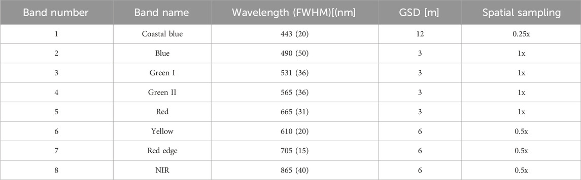
Table 1. SuperDove’s (SD) spectral bands, wavelengths, full-width half maximum (FWHM), ground sampling distance (GSD) and spatial sampling.
To exploit the SD observations more effectively, the quality (radiometric, spatial, spectral, and geometric) of the observations must be assessed and improved (Gordon, 1987; IOCCG, 2012; Kabir et al., 2020; Roy et al., 2017). Radiometric quality of SD observations is assessed and improved using vicarious techniques due to the lack of onboard calibrating instruments (e.g., shutter, lamp, solar diffuser). In practice, SD sensors are calibrated over terrestrial sites, every 6 months (January 1st and July 1st) using near-simultaneous observations with S2/MSI and validated with Radiometric Calibration Network (RadCalNet) (Collison et al., 2021). SD’s absolute/relative radiometric performance is evaluated occasionally. For instance, Saunier and Cocevar (2022, pg. 52) reported 0.4%–6.7% top-of-atmosphere (TOA) reflectance (
Firstly, this work presents the signal-to-noise ratio (SNR) assessment of SD bands over aquatic environments, which allows evaluation of the noise characteristics of SD images. This work further aimed to cross-calibrate SD sensors with S2/MSI using near-simultaneous observations over aquatic ecosystems. Here, S2/MSI was exploited as a reference sensor to cross-calibrate and improve the SD constellation due to their nearly overlapping spectral bands (five bands) (Tu et al., 2022). Specifically, we aimed to cross-compare the SD sensors’
This manuscript is structured as follows. Section 2 presents materials and methods which elaborate on the dataset, SNR assessment techniques,
2 Materials and methods
This section a) presents the dataset used for cross-calibration and validation (Section 2.1), b) explains SNR analysis technique (Section 2.2), c) describes cross-calibration and validation methods (Section 2.3), d) delineates
2.1 Dataset
Near-simultaneous SD-MSI observations, collected within 10 min, were searched globally over water bodies exploiting Planet Labs (hereafter Planet) application programming interface (API) (https://docs.planet.com/data/) and European Space Agencies (ESA) Copernicus Data Space Ecosystem (CDSE) API ((https://dataspace.copernicus.eu/). Access to the Planet’s API was provided under NASA’s Commercial Smallsat Data Acquisition (CSDA) program (NASA Earth Science Division, 2020), and ESA CDSE API was openly available. Firstly, SD-MSI image pairs were searched and identified from July 2023 to December 2023, and they are referred to as “calibration data.” This time frame was selected to align with Planet’s calibration cycle and to ensure consistent sensor behavior following routine quarterly updates and maintenance, as recommended in Planet’s guidelines (Collison et al., 2021). Then SD-MSI image pairs, collected from January 2024 to May 2024, were searched, and they are referred to as “validation data”. PlanetScope SD orthorectified images were downloaded from Planet’s API and S2/MSI L1C products were downloaded from CSDE API. Each downloaded SD orthorectified image consists of a scaled TOA radiance file, a metadata file, and a usable data mask (UDM2) file (Team, 2023).
2.2 Signal-to-noise ratio assessments
To investigate the random and/or systematic noises in the SD observations, SNRs of SD images were estimated from
2.3 Cross-calibration and validation
SD sensors were cross-calibrated and validated with MSI observations collected over global water bodies within 10 min of one another. Best practices were followed for identifying ideal matchup sites such that the difference between the observations is primarily due to their absolute radiometry. This cross-calibration was performed for the five common bands of SD and MSI (coastal blue (443 nm), blue (490 nm), green (565 nm), red (665 nm), and red-edge (705 nm)). The cross-calibration and validation was performed individually for each band. Note that SD TOA reflectance observations are operationally calibrated with MSI as a reference, suggesting that the SD and MSI observations should be directly comparable (Collison et al., 2021); hence, no spectral band adjustment has been performed throughout this study. Note also that the relative spectral response (RSR) of SD and MSI is nearly identical (Tu et al., 2022), and RSR-related differences are assumed to be negligible.
The procedure to identify suitable regions of interests (ROIs) to cross-calibrate and validate SD observations with MSI observations was as follows.
1. Convert SD and MSI observations to
2. Mask SD and MSI images. SD images were masked for cloud, cloud shadow, and haze using the provided UDM2 mask (Team, 2023). SD and MSI images were further filtered for clouds, cloud shadows, sun glint, and land pixels using ACOLITE AC processor-generated L2 flags (Vanhellemont, 2023; 2019b).
3. Generate per-pixel MSI angle files for each band. Per-pixel viewing zenith angles (VZA) viewing azimuth angles (VAA), SZA, and SAA were generated for each MSI band following the procedure presented in Pahlevan et al. (2017b). Note that SD images come with a single image center VZA, VAA, SZA, and SAA for each image.
4. Identify ideal matchups in the SD and MSI image pairs. Ideal matchups were defined as regions where differences in the angles (VZA, VAA) are minimal. To eliminate extreme off-nadir matchups, we discarded SD images and MSI pixels where VZA is
5. Locate homogenous ROIs in the MSI image. We calculated SNR within 7x7-element windows (all the pixels were valid) in MSI
6. Eliminate the outer-edge pixels from each 7 × 7 (square) window of MSI. SD’s absolute geolocation accuracy is ∼14 m, which means the SD pixel offset could be ∼five pixels (Semple et al., 2023). Moreover, signals originating from neighboring inhomogeneous pixels (i.e., edge pixel effect) and spatial resolution mismatches can reduce data consistency. To mitigate these impacts, two outer-edge pixels from the 7 × 7 square window were discarded and noted coordinates were used to calculate the average
7. Discard inhomogeneous matchup sites. The spatial homogeneity in MSI and SD
The above-explained matchup selection criteria were applied to the original full set of potential calibration (∼4000 SD images) and validation (∼2500 SD images) data. Following this screening process, 188 calibration SD images (60 MSI images) and 119 validation SD images (40 MSI images) remained to obtain cross-calibration parameters and validate the analysis, respectively. Figure 1 presents the global distribution of the calibration SD images (red squares) and validation SD images (green triangles), which includes different types of water bodies. Approximately 80% of the selected matchups are distributed across coastal regions, with the remaining 10% each covering inland and open ocean waters. This distribution reflects the greater availability of near-simultaneous SD-MSI observations over coastal areas, likely due to their proximity to land, higher revisit frequency, and increased likelihood of cloud-free scenes. The SNR estimation and calibration procedures exhibited linear computational complexity.
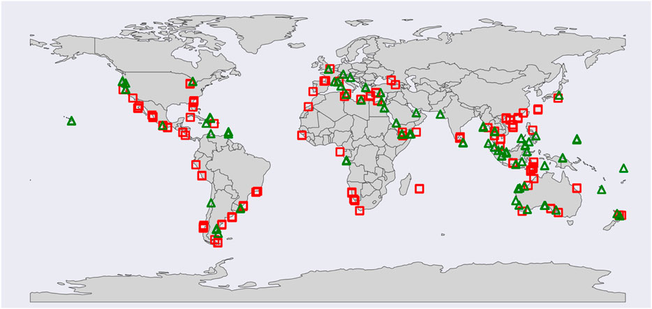
Figure 1. SuperDove (SD) - Multispectral Imager (MSI) near-simultaneous image pairs, including only the intercomparison regions that passed all the exclusion criteria. Red squares denote the 188-cross-calibration SD data and green triangles show the 119-validation SD data (not drawn to scale). The cross-calibration and validation datasets were distributed over different water bodies, including inland, coastal, and open oceans. Background map is obtained from Python’s ‘geopandas mapping and plotting tools’ library (https://geopandas.org/en/v0.9.0/docs/user_guide/mapping.html).
2.4 Remote sensing reflectance (
The remote sensing reflectance (
2.5 Water quality products
To demonstrate the value of these SD observations for WQ monitoring, particularly when combined with other satellite-based observations, we employed a machine learning (ML)-based mixture density network estimator (Pahlevan et al., 2022) to compare WQ indicators, such as
2.6 Performance metrics
SD observations were cross-calibrated with MSI data using ordinary least square linear regression (OLSLR) for the five SD-MSI bands. Slopes and intercepts from the OLSLR fit are the calibration gains and offsets, which are referred to as “calibration parameters”. To evaluate the agreements/discrepancies between SD-MSI before and after applying calibration parameters, the following metrics were also computed.
Differences in the MSI and SD products are expressed as percentage differences (
where
RMSD and bias were computed as follows:
where
The median difference (MD) was also calculated as below:
Due to the presence of noise in the analyses, the median metric was preferred over mean. The inter-consistency of MSI and SD products were gauged with these metrics, OLSLR statistics, including slope and intercept, and the coefficient of determination (R2).
3 Results
3.1 Signal-to-noise ratio assessments
SD SNRs computed from
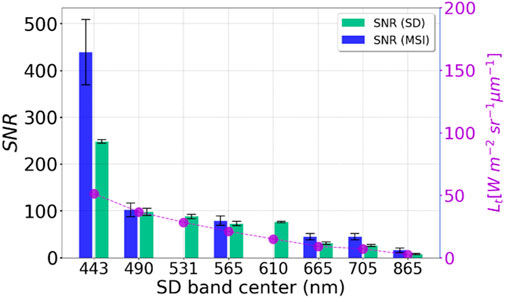
Figure 2. Bar graph comparing the signal-to-noise ratio (SNR) of multispectral imager (MSI) and SuperDove (SD) across various SD band centers in nanometers. SD SNRs estimated from seven SD images originating from six different SD instruments over Crater Lake in Oregon. The SNR for MSI is depicted in blue bars, while SD is shown in green bars. The SNR values generally decrease as the wavelength increases from 443 to 865 nm. A magenta line with circles indicates spectral radiance (Lt) along the right y-axis. Error bars are present for both SD and MSI readings.
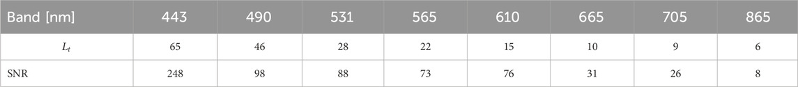
Table 2. SuperDove (SD) signal-to-noise ratios (SNRs) for the visible and near infrared (NIR) band.
3.2 Cross-calibration and validation
3.2.1 Cross-calibration
The SD-MSI differences in unitless
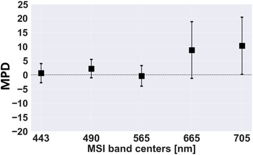
Figure 3. SuperDove (SD) and Multispectral Imager (MSI) top-of-atmosphere (TOA) reflectance (
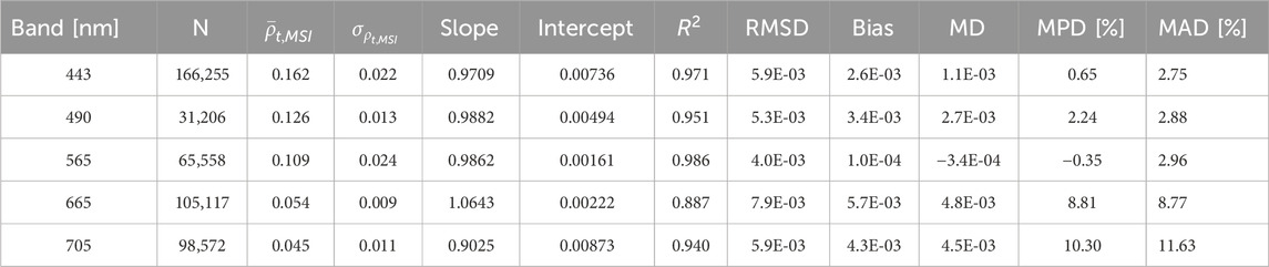
Table 3. The SuperDove (SD) - Multispectral Imager (MSI) top-of-atmosphere (TOA) reflectance (
3.2.2 Validation
The SD-MSI differences in
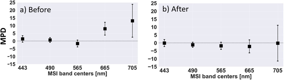
Figure 4. SuperDove (SD) and Multispectral Imager (MSI) top-of-atmosphere (TOA) reflectance (
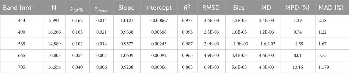
Table 4. The SuperDove (SD) – Multispectral Imager (MSI) top-of-atmosphere (TOA) reflectance (
Calibration parameters (i.e., slopes/gains and intercepts/offsets) developed in section 3.2.1 (refer to Table 3) were then applied to the validation SD
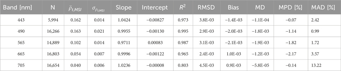
Table 5. The SuperDove (SD) - Multispectral Imager (MSI) top-of-atmosphere (TOA) reflectance (
3.3 Remote sensing reflectance (
The primary objective of this section is to evaluate the SD
3.3.1 Quantitative remote sensing reflectance (
The MPD in SD-MSI
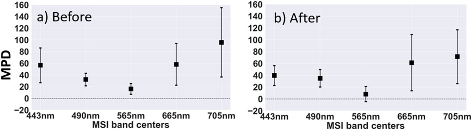
Figure 5. SD and MSI remote sensing reflectance (
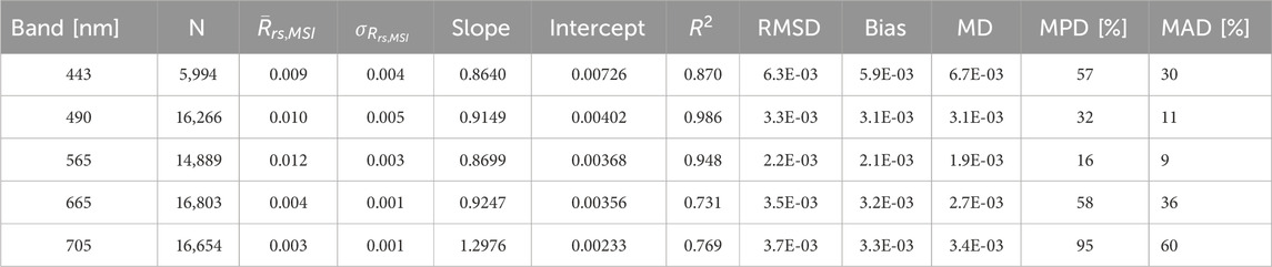
Table 6. The SuperDove (SD) - Multispectral Imager (MSI) remote sensing reflectance (
The consistency in SD-MSI
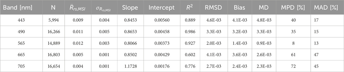
Table 7. The SuperDove (SD) - Multispectral Imager (MSI) remote sensing reflectance (
3.3.2 Qualitative
To visualize the differences in the ACOLITE-derived SD-MSI
Figure 6 shows the
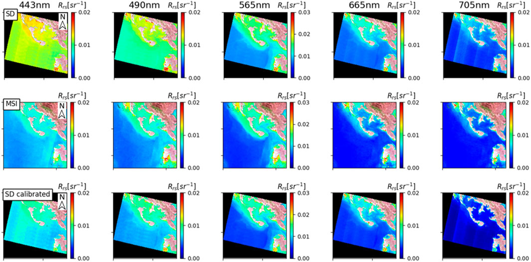
Figure 6. SuperDove (SD) and Multispectral Imager (MSI) remote sensing reflectance (
To further demonstrate the
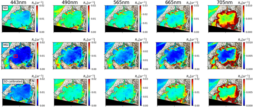
Figure 7. ACOLITE-derived SuperDove (SD) and Multispectral Imager (MSI) remote sensing reflectance (
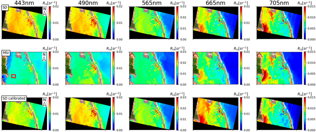
Figure 8. ACOLITE-derived SuperDove (SD) and Multispectral Imager (MSI) remote sensing reflectance (
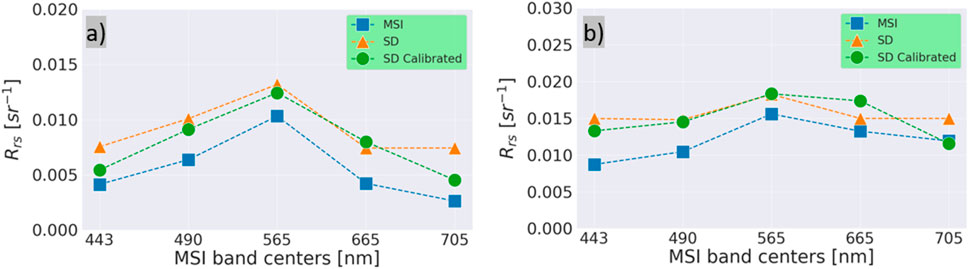
Figure 9. Mean SuperDove (SD) and Multispectral Imager (MSI) remote sensing reflectance (
Overall, the qualitative visual comparisons presented in Section 3.3.2 were largely consistent with the quantitative assessment in Section 3.3.1, particularly for bands 443, 565, and 705 nm, which showed notable improvements after calibration. However, minor discrepancies were observed in a few scenes, likely due to inherent uncertainties in the ACOLITE atmospheric correction process, such as view angle differences or sensor striping artifacts (refer to Section 4 for further discussion).
3.4 Water quality products
This section investigates the effect of calibration on the water quality (WQ) maps—specifically Chla and
3.4.1 Visual assessments
In this section, we present a qualitative comparison of SD and SD-cal derived WQ maps to the near-simultaneous MSI-derived WQ maps to get a general sense of the SD model’s ability to generate quality downstream products for WQ monitoring. The WQ maps for Boodalan Nature Reserve (Western Australia), Lake Almanor (California, United States), and Chesapeake Bay (eastern United States) are shown in Figures 10–12, respectively.
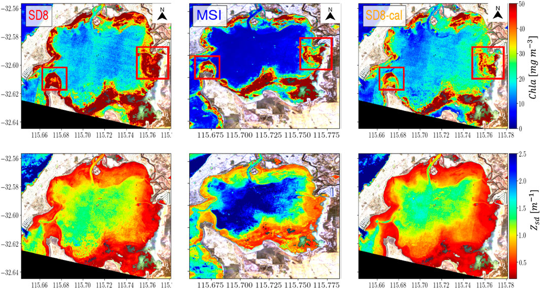
Figure 10. Effect of calibration on mixture density network (MDN) generated Chla (top row) and Secchi-disk-depth (
The Chla for Boodalan Nature Reserve (top row of Figure 10) shows consistent spatial trends across all three maps, with heightened Chla in nearshore regions but lower Chla at the center of the waterbody. The uncalibrated SD maps show consistently higher values than the MSI maps in both nearshore and central areas. Further, there are also differences in the spatial trends in the nearshore regions (especially in the regions highlighted by the red boxes). Post-calibration, these spatial differences were substantially diminished, even the central Chla values for the calibrated map are moderately suppressed and more in agreement with the MSI maps. However, the
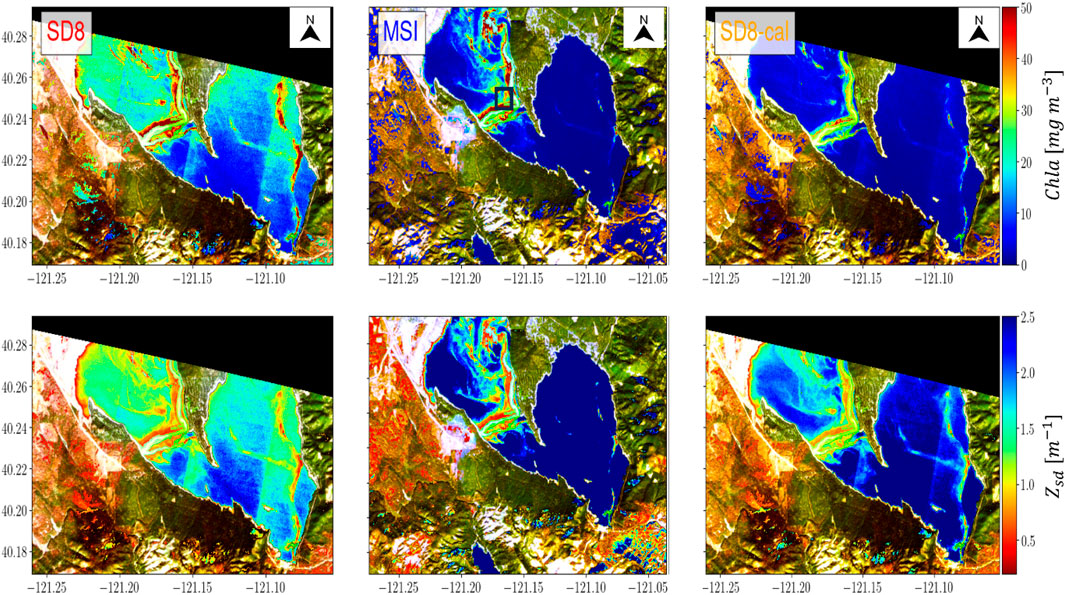
Figure 11. Effect of calibration on mixture density network (MDN) generated Chla (top row) and Secchi-disk-depth (
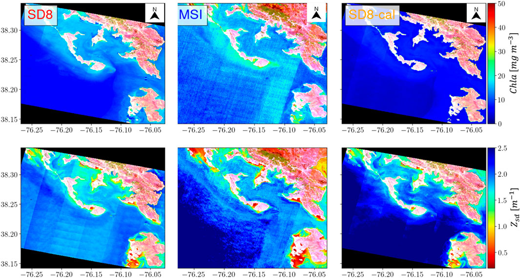
Figure 12. Effect of calibration on mixture density network (MDN) generated Chla (top row) and Sechhi-disk-depth (
Post-calibration, the spatial trends for the various WQI from both products generally agree more than before calibration. While this appears to be true based on our qualitative analysis, this may not always be the case. An example where the calibration does not seem to suppress the differences between the MSI and SD-generated WQ products is shown in Figure 12 for maps of Chesapeake Bay. Again, while there is general agreement regarding higher Chla and lower
3.4.2 Time-series analysis
To further demonstrate the utility of SD observations and MDN derived WQ parameters, we processed SD imagery that captured the impact of the Dixie Fire near Lake Almanor in California (https://www.fire.ca.gov/incidents/2021/7/13/dixie-fire). This wildfire event (started on 13 July 2021, and was fully contained on 25 Oct 2021) is known as the single largest wildfire in California history, which burned along the western shore of Lake Almanor. The Dixie Fire was immediately followed by eight inches of rainfall in just a few days in late Oct, which appeared to trigger an algal bloom in the lake (https://www.plumasnews.com/drought-and-dixie-fire-impacts-water-quality-at-lake-almanor/). The WQ product retrieval models, presented in Section 2.5 and inSupplementary Appendix C, were applied to SD observations (corrected with ACOLITE) to map Chla and
Figure 13 showcases the potential of SD observations to monitor water quality in Lake Almanor in the form of a time series. This time-series analysis serves to illustrate the feasibility of using cross-calibrated SD observations for tracking short-term water quality dynamics. We processed available SD and MSI observations over the lake from September 15 to 20 Dec 2021, and plotted average Chla and
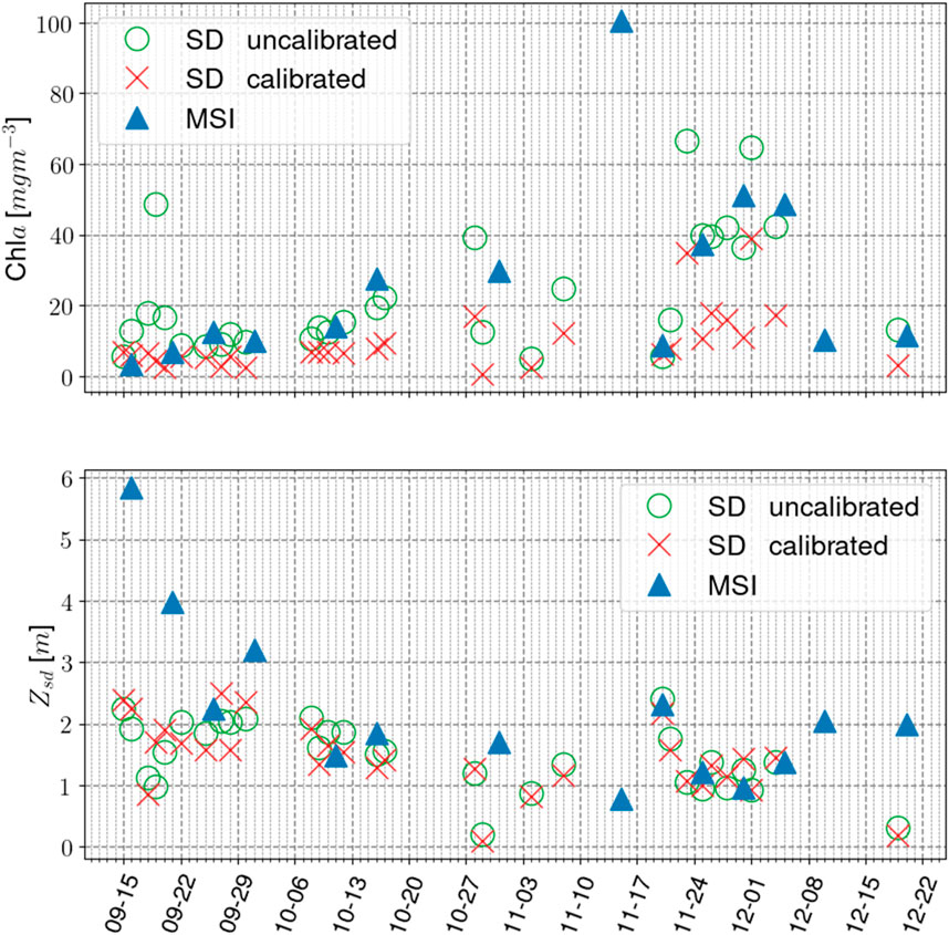
Figure 13. SuperDove (SD) and Multispectral Imager (MSI) Chla (top row) and Sechhi-disk-depth (
4 Discussions and future directions
We have presented the SNR assessment for the SD sensors to evaluate the noise performance (refer to Figure 2), including MSI SNRs reported in the literature. SD SNRs was slightly less than MSI for most of the bands (490, 565, 665 and 705 nm), whereas SD SNR for 443 nm is ∼0.5× of MSI SNR. Lower SNRs in the SD might be partly due to their finer spatial resolution compared to MSI. In this work, we assumed the sensor sensitivity or SNR of different SD instruments were similar, which may need further investigation. To characterize the noise of different SD instrument-generated images, SNRs ideally should be evaluated sensor-by-sensor. Moreover, we examined the SNRs over clear water in Crater Lake, Oregon due to the lack of open ocean observations. Ideally, SNRs should be evaluated over different aquatic and atmospheric conditions, as precision in water quality products (e.g., Chla, Zsd, etc.) depends on the noise performance of the observations (Hu et al., 2001, 2012).
We attempted to cross-calibrate the SD constellation with near-simultaneous MSI observations over a broad range of aquatic ecosystems, with the aim of developing calibration coefficients for SD images. The cross-calibration and validation of the SD constellation showed that our calibration parameters reduced the differences in SD and MSI
A fundamental limitation arises from the instability and inconsistencies across the multiple SD sensors. The PlanetScope constellation includes over 200 SD units, each exhibiting slight variations in radiometric behavior. Our analysis focused on a subset of 11 SD units, selected to be representative of the broader constellation in terms of geographic distribution and sensor behavior, while also keeping the analysis tractable. We observed substantial per-sensor variability in the relative differences between SD and MSI
We have also evaluated the ACOLITE-derived SD
The uncertainties in the cross-calibration and validation could arise from several different sources, including RSR function adjustment, spatial resolution mismatch, cloud, cloud shadow, and haze related noises, sun/sky glint, land-water adjacency effect, and high aerosol loading. This study assumed the RSR function related SD-MSI difference to be minimal since SD TOA reflectance products are calibrated to MSI TOA reflectance before disseminating SD data to the user (P. Team, 2022) and that the RSR of SD and MSI are nearly identical (Tu et al., 2022). However, future studies should investigate the RSR related differences in the
To demonstrate the potential of SD observations for aquatic science and applications, we applied ML based MDN models to retrieve Chla and
5 Summary and conclusion
This study described the radiometric cross-calibration and validation of SD
Data availability statement
The data analyzed in this study is subject to the following licenses/restrictions: The commercial Planet SuperDove satellite is subject to data availability and access regulations. Requests to access these datasets should be directed to https://csdap.earthdata.nasa.gov/.
Author contributions
SK: Investigation, Software, Methodology, Formal Analysis, Data curation, Visualization, Writing – original draft. AS: Writing – review and editing, Software. BB: Writing – review and editing. AA: Writing – review and editing, Project administration. RO’S: Writing – review and editing. VS: Writing – review and editing.
Funding
The author(s) declare that financial support was received for the research and/or publication of this article. This project was funded by NASA’s Commercial Smallsat Data Scientific Analysis (CSDA) program, grant # 80NSSC24K0049.
Acknowledgments
We acknowledge Nima Pahlevan (NASA Headquarters) and Keith Bouma-Gregson (USGS) for their contributions to the development of this study. Any use of trade, product, or firm names is for descriptive purposes only and does not imply endorsement by the U.S. Government.
Conflict of interest
Authors SK, AS, AA, RO’S were employed by Science Systems and Applications, Inc.
The remaining authors declare that the research was conducted in the absence of any commercial or financial relationships that could be construed as a potential conflict of interest.
Generative AI statement
The author(s) declare that no Generative AI was used in the creation of this manuscript.
Publisher’s note
All claims expressed in this article are solely those of the authors and do not necessarily represent those of their affiliated organizations, or those of the publisher, the editors and the reviewers. Any product that may be evaluated in this article, or claim that may be made by its manufacturer, is not guaranteed or endorsed by the publisher.
Supplementary material
The Supplementary Material for this article can be found online at: https://www.frontiersin.org/articles/10.3389/frsen.2025.1624783/full#supplementary-material
References
Balasubramanian, S. V., O’Shea, R. E., Saranathan, A. M., Begeman, C. C., Gurlin, D., Binding, C., et al. (2025). Mixture density networks for re-constructing historical ocean-color products over inland and coastal waters: demonstration and validation. Front. Remote Sens. 6, 1488565. doi:10.3389/frsen.2025.1488565
Balasubramanian, S. V., Pahlevan, N., Smith, B., Binding, C., Schalles, J., Loisel, H., et al. (2020). Robust algorithm for estimating total suspended solids (TSS) in inland and nearshore coastal waters. Remote Sens. Environ. 246, 111768. doi:10.1016/j.rse.2020.111768
Barnes, B. B., Hu, C., Bailey, S. W., Pahlevan, N., and Franz, B. A. (2021). Cross-calibration of MODIS and VIIRS long near infrared bands for ocean color science and applications. Remote Sens. Environ. 260, 112439. doi:10.1016/j.rse.2021.112439
Bulgarelli, B., Kiselev, V., and Zibordi, G. (2014). Simulation and analysis of adjacency effects in coastal waters: a case study. Appl. Opt. 53, 1523–1545. doi:10.1364/ao.53.001523
Caballero, I., and Stumpf, R. P. (2019). Retrieval of nearshore bathymetry from Sentinel-2A and 2B satellites in south Florida coastal waters. Estuar. Coast Shelf Sci. 226, 106277. doi:10.1016/j.ecss.2019.106277
Cao, Z., Ma, R., Liu, M., Duan, H., Xiao, Q., Xue, K., et al. (2022). Harmonized chlorophyll-a retrievals in inland lakes from Landsat-8/9 and Sentinel 2A/B virtual constellation through machine learning. IEEE Trans. Geoscience Remote Sens. 60, 1–16. doi:10.1109/tgrs.2022.3207345
Collison, A., Jumpasut, A., and Bourne, H. (2021). On-Orbit Radiometric Calibration of the planet satellite fleet. Available online at: https://assets.planet.com/docs/radiometric_calibration_white_paper.pdf (Accessed July 24, 2025).
De Keukelaere, L., Sterckx, S., Adriaensen, S., Knaeps, E., Reusen, I., Giardino, C., et al. (2018). Atmospheric correction of Landsat-8/OLI and Sentinel-2/MSI data using iCOR algorithm: validation for coastal and inland waters. Eur. J. Remote Sens. 51, 525–542. doi:10.1080/22797254.2018.1457937
Fernandez-Saldivar, J., Pritchett, C., Ozawa, K., and Zuleta, I. (2020). Focus characterization of SuperDoves: On-ground and On-orbit first light.
Fickas, K. C., O’Shea, R. E., Pahlevan, N., Smith, B., Bartlett, S. L., and Wolny, J. L. (2023). Leveraging multimission satellite data for spatiotemporally coherent cyanoHAB monitoring. Front. Remote Sens. 4, 1157609. doi:10.3389/frsen.2023.1157609
Frazier, A. E., and Hemingway, B. L. (2021). A technical review of planet smallsat data: practical considerations for processing and using planetscope imagery. Remote Sens. (Basel) 13, 3930. doi:10.3390/rs13193930
Gilerson, A., Carrizo, C., Foster, R., and Harmel, T. (2018). Variability of the reflectance coefficient of skylight from the ocean surface and its implications to ocean color. Opt. Express 26, 9615–9633. doi:10.1364/oe.26.009615
Gordon, H. R. (1987). Calibration requirements and methodology for remote sensors viewing the ocean in the visible. Remote Sens. Environ. 22, 103–126. doi:10.1016/0034-4257(87)90029-0
Gordon, H. R., Du, T., and Zhang, T. (1997). Remote sensing of ocean color and aerosol properties: resolving the issue of aerosol absorption. Appl. Opt. 36, 8670–8684. doi:10.1364/ao.36.008670
Hu, C., Carder, K. L., and Muller-Karger, F. E. (2001). How precise are SeaWiFS ocean color estimates? Implications of digitization-noise errors. Remote Sens. Environ. 76, 239–249. doi:10.1016/s0034-4257(00)00206-6
Hu, C., Feng, L., Lee, Z., Davis, C. O., Mannino, A., McClain, C. R., et al. (2012). Dynamic range and sensitivity requirements of satellite ocean color sensors: learning from the past. Appl. Opt. 51, 6045–6062. doi:10.1364/ao.51.006045
IOCCG (2012). Mission requirements for future ocean-colour sensors. Dartmouth, NS: Reports of the International Ocean-Colour Coordinating Group.
Jumpasut, A., Collison, A., and Zuleta, I. (2020). On-orbit validation of interoperability between Planet SuperDoves and Sentinel-2.
Kabir, S., Leigh, L., and Helder, D. (2020). Vicarious methodologies to assess and improve the quality of the optical remote sensing images: a critical review. Remote Sens. (Basel) 12, 4029. doi:10.3390/rs12244029
Kabir, S., Pahlevan, N., O’Shea, R. E., and Barnes, B. B. (2023). Leveraging Landsat-8/-9 underfly observations to evaluate consistency in reflectance products over aquatic environments. Remote Sens. Environ. 296, 113755. doi:10.1016/j.rse.2023.113755
Kuhn, C., de Matos Valerio, A., Ward, N., Loken, L., Sawakuchi, H. O., Kampel, M., et al. (2019). Performance of Landsat-8 and Sentinel-2 surface reflectance products for river remote sensing retrievals of chlorophyll-a and turbidity. Remote Sens. Environ. 224, 104–118. doi:10.1016/J.RSE.2019.01.023
Lavender, S. (2024). European Space Agency (ESA). Technical Note on Quality Assessment for Planet SuperDove. Available online at: https://earth.esa.int/documents/d/earth-online/technical-note-on-quality-assessment-for-superdove-apr-2024 (Accessed July 24, 2025).
Lee, Z., Shang, S., Qi, L., Yan, J., and Lin, G. (2016). A semi-analytical scheme to estimate Secchi-disk depth from Landsat-8 measurements. Remote Sens. Environ. 177, 101–106. doi:10.1016/j.rse.2016.02.033
Lewis, M. D., Jarreau, B., Jolliff, J., Ladner, S., Lawson, T. A., McCarthy, S., et al. (2023). Assessing planet nanosatellite sensors for Ocean color usage. Remote Sens. (Basel) 15, 5359. doi:10.3390/rs15225359
Li, J., and Chen, B. (2020). Global revisit interval analysis of Landsat-8-9 and Sentinel-2A-2B data for terrestrial monitoring. Sensors 20, 6631. doi:10.3390/s20226631
Maciel, D. A., Pahlevan, N., Barbosa, C. C. F., Martins, V. S., Smith, B., O’Shea, R. E., et al. (2023). Towards global long-term water transparency products from the Landsat archive. Remote Sens. Environ. 299, 113889. doi:10.1016/j.rse.2023.113889
McCarthy, S., Lewis, M. D., Lawson, A., Martinolich, P., Jolliff, J. K., and Ladner, S. (2023). “Current Ocean color processing capabilities of planet’s nanosatellite data within nrl’s automated processing System,” in OCEANS 2023-MTS/IEEE US Gulf Coast. Biloxi, MS: IEEE, 1–6.
Mobley, C. D. (1999). Estimation of the remote-sensing reflectance from above-surface measurements. Appl. Opt. 38 (36), 7442–7455. doi:10.1364/ao.38.007442
NASA Earth Science Division (2020). Commercial Smallsat Data Acquisition Program (CSDAP). Commercial smallsat data evaluation report. NASA Earthdata. Available online at: https://www.earthdata.nasa.gov/s3fs-public/imported/CSDAPReport0420.pdf.
Niroumand-Jadidi, M., Legleiter, C. J., and Bovolo, F. (2022). River bathymetry retrieval from Landsat-9 images based on neural networks and comparison to SuperDove and Sentinel-2. IEEE J. Sel. Top. Appl. Earth Obs. Remote Sens. 15, 5250–5260. doi:10.1109/jstars.2022.3187179
Pacheco, A., Horta, J., Loureiro, C., and Ferreira, Ó. (2015). Retrieval of nearshore bathymetry from Landsat 8 images: a tool for coastal monitoring in shallow waters. Remote Sens. Environ. 159, 102–116. doi:10.1016/j.rse.2014.12.004
Pahlevan, N., Mangin, A., Balasubramanian, S. V., Smith, B., Alikas, K., Arai, K., et al. (2021). ACIX-Aqua: a global assessment of atmospheric correction methods for Landsat-8 and Sentinel-2 over lakes, rivers, and coastal waters. Remote Sens. Environ. 258, 112366. doi:10.1016/J.RSE.2021.112366
Pahlevan, N., Balasubramanian, S., Begeman, C. C., O’Shea, R. E., Ashapure, A., Maciel, D. A., et al. (2024). A retrospective analysis of remote-sensing reflectance products in coastal and inland waters. IEEE Geoscience Remote Sens. Lett. 21, 1–5. doi:10.1109/lgrs.2024.3351328
Pahlevan, N., Chittimalli, S. K., Balasubramanian, S. V., and Vellucci, V. (2019). Sentinel-2/Landsat-8 product consistency and implications for monitoring aquatic systems. Remote Sens. Environ. 220, 19–29. doi:10.1016/J.RSE.2018.10.027
Pahlevan, N., Lee, Z., Wei, J., Schaaf, C. B., Schott, J. R., and Berk, A. (2014). On-orbit radiometric characterization of OLI (Landsat-8) for applications in aquatic remote sensing. Remote Sens. Environ. 154, 272–284. doi:10.1016/J.RSE.2014.08.001
Pahlevan, N., Sarkar, S., Franz, B. A., Balasubramanian, S. V., and He, J. (2017a). Sentinel-2 MultiSpectral Instrument (MSI) data processing for aquatic science applications: demonstrations and validations. Remote Sens. Environ. 201, 47–56. doi:10.1016/J.RSE.2017.08.033
Pahlevan, N., Schott, J. R., Franz, B. A., Zibordi, G., Markham, B., Bailey, S., et al. (2017b). Landsat 8 remote sensing reflectance (Rrs) products: evaluations, intercomparisons, and enhancements. Remote Sens. Environ. 190, 289–301. doi:10.1016/J.RSE.2016.12.030
Pahlevan, N., Smith, B., Alikas, K., Anstee, J., Barbosa, C., Binding, C., et al. (2022). Simultaneous retrieval of selected optical water quality indicators from Landsat-8, Sentinel-2, and Sentinel-3. Remote Sens. Environ. 270, 112860. doi:10.1016/J.RSE.2021.112860
Pahlevan, N., Smith, B., Schalles, J., Binding, C., Cao, Z., Ma, R., et al. (2020). Seamless retrievals of chlorophyll-a from Sentinel-2 (MSI) and Sentinel-3 (OLCI) in inland and coastal waters: a machine-learning approach. Remote Sens. Environ. 240, 111604. doi:10.1016/j.rse.2019.111604
Pitarch, J., and Vanhellemont, Q. (2021). The QAA-RGB: a universal three-band absorption and backscattering retrieval algorithm for high resolution satellite sensors. Development and implementation in ACOLITE. Remote Sens. Environ. 265, 112667. doi:10.1016/j.rse.2021.112667
Roy, P. S., Behera, M. D., and Srivastav, S. K. (2017). Satellite remote sensing: sensors, applications and techniques. Proc. Natl. Acad. Sci. India Sect. A Phys. Sci. 87, 465–472. doi:10.1007/s40010-017-0428-8
Semple, A. G., Tan, B., and Lin, G.Gary (2023). SuperDove geometric quality assessment summary. Greenbelt, MD.
Smith, B., Pahlevan, N., Schalles, J., Ruberg, S., Errera, R., Ma, R., et al. (2021). A chlorophyll-a algorithm for Landsat-8 based on mixture density networks. Front. Remote Sens. 1, 623678. doi:10.3389/frsen.2020.623678
Steinmetz, F., and Ramon, D. (2018). “Sentinel-2 MSI and Sentinel-3 OLCI consistent ocean colour products using POLYMER,” in Remote sensing of the open and coastal Ocean and inland waters (Honolulu, HI: SPIE), 46–55.
Tu, Y.-H., Johansen, K., Aragon, B., El Hajj, M. M., and McCabe, M. F. (2022). The radiometric accuracy of the 8-band multi-spectral surface reflectance from the planet SuperDove constellation. Int. J. Appl. Earth Observation Geoinformation 114, 103035. doi:10.1016/j.jag.2022.103035
USGS (2020). Commercial smallsat data acquisition program system characterization report for PlanetScope SuperDove instruments. U.S. Geological Survey. Available online at: https://www.earthdata.nasa.gov/s3fs-public/imported/CSDAPReport0420.pdf (Accessed July 24, 2025).
Vanhellemont, Q. (2019a). Daily metre-scale mapping of water turbidity using CubeSat imagery. Opt. Express 27, A1372–A1399. doi:10.1364/oe.27.0a1372
Vanhellemont, Q. (2019b). Adaptation of the dark spectrum fitting atmospheric correction for aquatic applications of the landsat and Sentinel-2 archives. Remote Sens. Environ. 225, 175–192. doi:10.1016/J.RSE.2019.03.010
Vanhellemont, Q. (2023). Evaluation of eight band SuperDove imagery for aquatic applications. Opt. Express 31, 13851–13874. doi:10.1364/oe.483418
Vanhellemont, Q., and Ruddick, K. (2014). Turbid wakes associated with offshore wind turbines observed with landsat 8. Remote Sens. Environ. 145, 105–115. doi:10.1016/J.RSE.2014.01.009
Vanhellemont, Q., and Ruddick, K. (2018). Atmospheric correction of metre-scale optical satellite data for inland and coastal water applications. Remote Sens. Environ. 216, 586–597. doi:10.1016/j.rse.2018.07.015
Wang, D., Ma, R., Xue, K., and Loiselle, S. A. (2019). The assessment of Landsat-8 OLI atmospheric correction algorithms for inland waters. Remote Sens. (Basel) 11, 169. doi:10.3390/rs11020169
Wang, M. (2010). IOCCG, “atmospheric correction for remotely-sensed ocean-colour products”. Dartmouth, NS: Reports of the International Ocean-Colour Coordinating Group.
Warren, M. A., Simis, S. G. H., Martinez-Vicente, V., Poser, K., Bresciani, M., Alikas, K., et al. (2019). Assessment of atmospheric correction algorithms for the Sentinel-2A MultiSpectral imager over coastal and inland waters. Remote Sens. Environ. 225, 267–289. doi:10.1016/J.RSE.2019.03.018
Wei, J., Lee, Z., Garcia, R., Zoffoli, L., Armstrong, R. A., Shang, Z., et al. (2018). An assessment of Landsat-8 atmospheric correction schemes and remote sensing reflectance products in coral reefs and coastal turbid waters. Remote Sens. Environ. 215, 18–32. doi:10.1016/j.rse.2018.05.033
Zhang, X., Wang, L., Li, J., Han, W., Fan, R., and Wang, S. (2023). Satellite-derived sediment distribution mapping using ICESat-2 and SuperDove. ISPRS J. Photogrammetry Remote Sens. 202, 545–564. doi:10.1016/j.isprsjprs.2023.06.009
Keywords: superdove, radiometry, signal-to-noise ratio, top-of-atmosphere (TOA) reflectance, remote sensing reflectance, inland/coastal waters, water quality
Citation: Kabir S, Saranathan AM, Barnes BB, Ashapure A, O’Shea RE and Stengel VG (2025) Feasibility of PlanetScope SuperDove constellation for water quality monitoring of inland and coastal waters. Front. Remote Sens. 6:1624783. doi: 10.3389/frsen.2025.1624783
Received: 07 May 2025; Accepted: 15 July 2025;
Published: 04 August 2025.
Edited by:
Sawaid Abbas, University of the Punjab, PakistanReviewed by:
Lewis McCaffrey, State of New York, United StatesChangpeng Li, Ministry of Natural Resources, China
Alba German, Instituto de Altos Estudios Espaciales Mario Gulich, Argentina
Copyright © 2025 Kabir, Saranathan, Barnes, Ashapure, O’Shea and Stengel. This is an open-access article distributed under the terms of the Creative Commons Attribution License (CC BY). The use, distribution or reproduction in other forums is permitted, provided the original author(s) and the copyright owner(s) are credited and that the original publication in this journal is cited, in accordance with accepted academic practice. No use, distribution or reproduction is permitted which does not comply with these terms.
*Correspondence: Akash Ashapure, YWthc2guYXNoYXB1cmVAbmFzYS5nb3Y=