Characterising the spatio-temporal patterns of water quality parameters in the cradle of humankind world heritage site using Sentinel-2 and random forest regressor

Introduction: Water quality assessment is essential for monitoring and managing freshwater resources, particularly in ecologically and culturally significant areas like the Cradle of Humankind World Heritage Site (COHWHS). This study aimed to predict and map the spatio-temporal patterns of both optically and non-optically active water quality parameters within small inland water bodies located in the COHWHS.

Methods: High-resolution Sentinel-2 Multispectral Instrument (MSI) satellite data and two random forest models (Model 1 [consisting of sensitive spectral bands] and Model 2 [consisting of spectral bands + indices]) were used alongside In-situ measurements of chlorophyll-a, suspended solids, dissolved oxygen (DO), pH, Temperature, and electrical conductivity (EC) were integrated to establish empirical relationships and assess spatial variability across high-flow and low-flow conditions.

Results: The results indicated that DO could be predicted with the highest accuracy under low-flow conditions, followed by EC. Specifically, Model 2 achieved an R² of 0.88 and an RMSE of 1.37 for DO, while Model 1 achieved an R² of 0.63 and an RMSE of 291.48 for EC. For optically active parameters, suspended solids showed the highest prediction accuracy under high-flow conditions using Model 2 (R²p = 0.55; RMSE = 118.19). Due to the over-pixelation of other smaller water bodies within the COHWHS in Sentinel-2 imagery, Cradlemoon Lake was selected to show distinct seasonal (high- and low-flow) and spatial variations in optically and non-optically active water quality parameters.

Discussion: Variations in the results were influenced by runoff dynamics and upstream pollution: lower Temperatures and suspended solids under low-flow conditions increased DO concentrations, whereas higher suspended solid concentrations under high-flow conditions likely reduced light penetration, resulting in lower spectral reflectance and chlorophyll-a levels. These findings highlight the potential of Sentinel-2 MSI data and machine learning models for monitoring dynamic water quality variations in freshwater ecosystems.

1 Introduction

Anthropogenic activities such as population growth, increasing urbanisation, intensive industrial development, and agriculture have increased the demand for and misuse of inland water bodies. This has, in turn, increased water stress and water quality deterioration, especially in various countries (Jakovljevic et al., 2024). Globally, water degradation has worsened throughout the years as about 80% of all industrial and domestic waste is transferred to water resources without any treatment, further degrading freshwater and making it unsafe for drinking and sanitation (du Plessis, 2022). Additionally, seasonal variations influence water quality by altering physical and chemical parameters, which can contribute to its deterioration. Fluctuations in Temperature, runoff, and pollutant inputs affect key indicators such as turbidity, dissolved oxygen, and nutrient levels, potentially degrading water quality and impacting aquatic ecosystems (Dey et al., 2021). Due to these reasons, there is a need for regular monitoring of physio-chemical parameters within inland water bodies to develop corrective measures that will contribute to the accomplishment of Sustainable Development Goal (SDG) 6, which aims for clean water and sanitation for all by 2030 (Sherjah et al., 2023; Jakovljevic et al., 2024). This can be achieved through water quality monitoring, which involves monitoring the biological, chemical, and physical characteristics of water, such as chlorophyll-a, suspended solids, dissolved oxygen, nitrogen and phosphorus (among others) (Sagan et al., 2020).

Water quality monitoring helps track changes in water quality across different areas, analyse seasonal patterns and assess the overall health of various water bodies (Madonsela et al., 2024). Traditionally, this process has relied on collecting water samples, conducting laboratory tests, and performing in situ measurements. However, these methods are limited in spatial and temporal coverage, making it challenging to monitor large areas and capture rapid changes in water quality (Jaji et al., 2007). Moreover, these methods are not cost-effective, as assessing spatio-temporal patterns requires frequent site visits, increasing logistical and financial demands (Zainurin et al., 2022; Adjovu et al., 2023; Ndou, 2023; Madonsela et al., 2024). Satellite sensors provide an opportunity to regularly monitor the spatio-temporal patterns of water quality parameters over large geographic areas. They offer efficient, cost-effective, and near real-time water quality assessments, enabling the remote identification of temporal trends and spatial hotspots (Dube et al., 2015; Pizani et al., 2020). Satellite sensors with low-medium spatial resolution and high temporal resolution have been used to monitor spatio-temporal patterns in water bodies, however, the challenge is how they may not be suitable for monitoring small inland water bodies (Mashala et al., 2023). Studies (Chavula et al., 2009; Arun Kumar et al., 2015; Shi et al., 2018; Xiong et al., 2019) have shown that the Moderate Resolution Imaging Spectroradiometer (MODIS) sensor, with a medium spatial resolution of 250 m–500 m–1 km and a high temporal resolution of 1–2 days, has been widely used to monitor water quality parameters on larger coastal and inland water bodies such as lakes and dams.

However, Wang et al. (2023), in their study on monitoring algal blooms in 171 lakes across China, noted that MODIS’s medium spatial resolution (500 m) limited their analysis to large lakes (>10 km²), while smaller lakes (∼1 km²) required higher-resolution sensors, such as the Sentinel-2 Multispectral Instrument (MSI). This highlights the need for medium- to high-resolution satellite sensors to address the limitations of low-resolution sensors such as MODIS. These sensors can enhance water quality monitoring in dynamic aquatic ecosystems, improving the estimation of spatio-temporal variations, especially in understudied small inland water bodies under different flow conditions (Ciężkowski et al., 2022). Since its launch, the Sentinel-2 MSI, with its fine spatial resolution (10 m–20 m) and frequent revisit time (every 5 days), has played a key role in monitoring water quality parameters. For example, Ciężkowski et al. (2022) demonstrated the advantages of using Sentinel-2 data for long-term spatio-temporal monitoring of water quality in the Głuszyńskie Lake since 2015. Their study found a strong correlation (R² > 0.75) between estimated water quality parameters - biological oxygen demand, dissolved organic carbon, and chlorophyll concentration - and in situ data, highlighting Sentinel-2’s reliability for monitoring temporal trends and spatial distributions. This satellite sensor provides an opportunity to assess spatiotemporal patterns of water quality parameters in smaller inland water bodies, such as rivers.

Techniques for mapping spatio-temporal patterns, have been dominated by spectral indices, which simplify and enhance the interpretation of complex information derived from their various spectral bands (Scordo et al., 2018; Ciężkowski et al., 2022). Spectral indices are mathematical formulas that combine satellite sensor bands to enhance specific features like vegetation or water (Hadibasyir et al., 2023; Mashala et al., 2023). Moreover, these indices use specific satellite bands that are sensitive to water quality parameters, making them useful for assessing parameters like turbidity, chlorophyll-a, and total suspended solids (Montero et al., 2023; Zhu et al., 2024). For instance, Abdulla Alserkal et al. (2024) aimed to estimate and map water quality parameters in the Al Rafisah Dam (United Arab Emirates), focusing on Chlorophyll-a, Colour Dissolved Organic Matter (CDOM), Total Suspended Matter (TSM), and turbidity across different seasons in 2021. Using Sentinel-2 data with the Normalized Difference Turbidity Index (NDTI - Red Band [B4] and Green Band [B3]), they found moderate turbidity concentrations with spatial hotspots in the southern and northern parts of the dam. Similarly, Mpakairi et al. (2024) applied the Normalized Difference Chlorophyll Index (NDCI - Red-Edge Band [B5] and Red Band [B4]) to estimate chlorophyll-a concentrations using Sentinel-2 spectral bands. Their study revealed that NDCI outperformed other indices in the Nandoni Reservoir (South Africa), effectively mapping chlorophyll concentration patterns in this subtropical reservoir. Furthermore, Kowe et al. (2023) used, Sentinel-2 data, the Normalized Difference Vegetation Index (NDVI) and empirical models to assess spatio-temporal variations (2017–2022) in Total Nitrogen, Turbidity, chlorophyll-a, and Total Suspended Solids in Lake Manyame, Zimbabwe, revealing significant fluctuations over time and strong correlations between satellite-derived and in situ data (R² = 0.63–0.95).

These previous studies (Ciężkowski et al., 2022; Kowe et al., 2023; Abdulla Alserkal et al., 2024; Mpakairi et al., 2024) demonstrate the use of Sentinel-2 MSI in capturing spatio-temporal patterns of water quality parameters and highlight how spectral indices enhance these estimations. However, these studies primarily focus on optically active water quality parameters, which are more frequently studied than non-optically active parameters. Non-optically active water quality parameters lack strong spectral signals and do not directly affect water reflectance, making them difficult to detect using optical sensors (Arias-Rodriguez et al., 2023). They are typically measured through in situ measurement or estimated using empirical models linked to optically active parameters (Guo et al., 2021a). Given Sentinel-2’s multispectral capabilities, high spatial and temporal resolution, and the effectiveness of spectral indices, it is essential to explore the integration of these techniques for monitoring the spatio-temporal patterns of non-optically active water quality parameters in small inland water bodies. However, since non-optically active parameters lack distinct spectral signals, their characterisation is challenging and often relies on their relationships with optically active parameters. To address this complexity, advanced analytical techniques such as machine learning models should be integrated into studies using Sentinel-2 data and spectral indices. This approach can enhance the reliability and accuracy of assessing the spatial and temporal dynamics of these parameters (Arias-Rodriguez et al., 2023; Tian et al., 2023).

Machine learning algorithms such as Decision Trees (DT), Random Forest Regression (RFR), Boosted Regression Trees (BRT), Support Vector Regression (SVR), and Artificial Neural Networks (ANN) have been widely applied in water quality assessment and monitoring because they can handle complex, non-linear relationships between water quality parameters and remote sensing data (Yahya et al., 2019; Li et al., 2022; Arif and Toersilowati, 2024; Barcia et al., 2024; Glinscaya et al., 2024). Machine learning algorithms, combined with satellite and in situ data, enhance spatial and temporal water quality monitoring beyond traditional sampling methods (Rodriguez-Galiano et al., 2012). Thus, selecting the optimal machine learning algorithm for capturing the complex relationships involved in monitoring non-optically active water quality parameters is crucial for accurate estimations. For instance, RFR has been recognised as one of the most effective machine learning algorithms for practical applications (Wang et al., 2021; Xu et al., 2021. It uses multiple decision trees to predict outcomes based on a set of predictors (Tyralis et al., 2019). Wang et al. (2021) developed and found a RFR model to be highly effective in predicting water quality parameters, outperforming other models such as Decision Tree Regression (DTR), AdaBoost Regression (ABR), Gradient Boosting Regression (GBR), Support Vector Regression (SVR), K-Nearest Neighbor (KNN), Artificial Neural Networks (ANN), Lasso Regression (LASSO), and Elastic Net Regression (ENR). Furthermore, Mpakairi et al. (2024) demonstrated the advantages of integrating RFR with spectral indices like the NDCI to enhance predictions of water quality parameter spatio-temporal patterns. This highlights the need to integrate Sentinel-2 data, in situ measurements, machine learning, spectral indices and satellite bands that are sensitive to water quality parameters to enhance spatio-temporal predictions of water quality parameters in small inland water bodies.

Against this background, this study aimed to evaluate the predictive performance of the Random Forest Regressor (RFR) in estimating both optically active and non-optically active water quality parameters under high-flow (wet) and low-flow (dry) conditions in the Cradle of Humankind World Heritage Site (COHWHS). This area experiences significant anthropogenic pressures, including Acid Mine Drainage (AMD) and effluent discharge from municipal wastewater treatment facilities, which adversely impact water resources (Mugova and Wolkersdorfer, 2022). To achieve this aim, the study designed two random forest regression (RFR) models: (1) Model 1, which included only the Sentinel-2 bands identified as sensitive to specific water quality parameters in our previous work (Ngamile et al., under review), providing a parameter-specific optimised modelling scenario; and (2) Model 2, which incorporated all Sentinel-2 spectral bands along with spectral indices, offering a more generalisable modelling scenario. Additionally, the study sought to identify the most influential variables for predicting optically active and non-optically active water quality parameters under both high-flow and low-flow conditions based on RFR variable importance. The optimal models were used to map the spatial and temporal distribution of water quality parameters in the COHWHS, South Africa. This study is the first to evaluate RFR’s performance in characterising water quality under different hydrological conditions in a semi-arid African region. The findings support the potential integration of Sentinel-2 data with machine learning for enhancing water quality monitoring and informing sustainable water resource management.

2 Materials and methods

2.1 Description of the study area

The Cradle of Humankind World Heritage Site (COHWHS) covers approximately 800 km² and is located 40 km northwest of Johannesburg in the West Rand District of Gauteng, South Africa (Durand et al., 2010). It was designated a UNESCO World Heritage Site in 1999 due to its rich paleoanthropological significance, featuring over 200 caves containing fossilised hominid remains (Durand et al., 2010). However, the COHWHS faces significant environmental challenges, particularly from acid mine drainage (AMD) associated with historical gold mining in the Western Witwatersrand Basin, which has severely impacted local water quality (Rogerson and van der Merwe, 2016). In addition, sewage effluent and agricultural runoff further contribute to the contamination and alteration of water chemistry in the area (Holland and Witthüser, 2009). These pollutants enter local rivers, such as the Tweelopiespruit and Blougatspruit, which flow downstream into the Bloubankspruit and, ultimately, the Crocodile River (as seen in Figure 1). The Crocodile River serves as a tributary and inflow zone for Cradlemoon Lake, making the lake susceptible to contamination from AMD, sewage effluent, and agricultural runoff. Furthermore, runoff from Cradlemoon Lake contributes to the pollution of larger water bodies, including the Hartbeespoort Dam and its surrounding areas, emphasizing the need for continuous water quality monitoring in the COHWHS (Hobbs, 2017). Given that locations like Cradlemoon Lake serve as tourist attractions and host various leisure activities, monitoring water quality is crucial to assessing potential health risks associated with water pollution in the COHWHS.

Figure 1

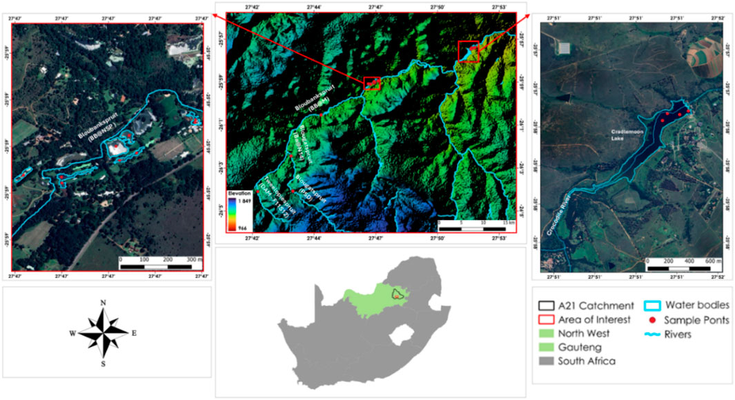
Figure 1. Map of the water bodies in and around the COHWHS.

2.2 Data collection

2.2.1 Water sampling and in-situ measurements

The in situ measurements of the water quality parameters occurred over two seasons, where wet season fieldwork, representing high-flow conditions, was performed between the 14th and 16th of March 2024 and dry season fieldwork, representing low-flow conditions, happened on the 28th and the 31st of August 2024. These dates were selected to correspond with the Satellite overpass of the Sentinel-2 Multi-Spectral Instrument (MSI) over the study area. In-situ measurements were taken between 09h00 SAST and 15h00 SAST to minimise the gap between the satellite overpass and in situ measurements. A total of 40 measurements of each water quality parameter (See Tables 1, 2) were taken from six sites, selected purposively, on the Tweelopiespruit (Dam [F11S12]), Blougatspruit (PSD and BB@N14), Bloubankspruit (BB@M and BB@NSP) and on the Cradlemoon Lake (as seen in Figure 1). The purposive sampling approach was used to choose specific sampling sites along the water bodies based on how well the data collected from them would best inform the study (Bhardwaj, 2019). Each sample was tagged with a GPS coordinate using the Garmin GPSMAP 65S handheld GPS device, which has a positional accuracy of ±3 m.

Table 1

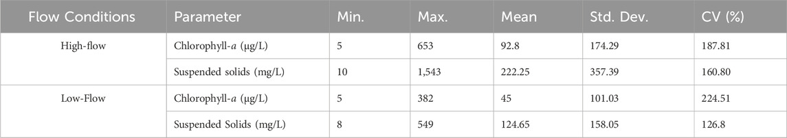
Table 1. Summary statistics of optically active water quality parameters during highflow and lowflow conditions.

Table 2

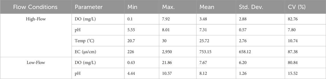
Table 2. Summary statistics of nonoptically active water quality parameters during highflow and lowflow conditions.

At each site, water samples (collected at depths ranging between 10 cm and 0.5 m for each site) and in situ measurements were collected. While the water samples were collected in 1 L plastic brown and transparent bottles for laboratory analysis to determine optically active parameters, i.e., chlorophyll-a and suspended solids concentrations, respectively, in situ measurement of non-optically active water quality parameters, i.e., Dissolved Oxygen (DO), pH, Temperature and Electrical Conductivity (EC), were obtained using the Hach HQ40d multiparameter meter (Hach, Loveland, Colorado, United States of America) using various probes designed to capture each parameter. While in the field, we preserved the condition of the water samples in the cooler box with ice cubes to maintain a low Temperature before transporting and storing the samples in a cold room of the Hydrology and Water Resources Laboratory of the Council for Scientific and Industrial Research (CSIR) at 4°C. A total of 40 samples were collected in each season.

2.2.2 Satellite data

Sentinel-2 Level 1C images, which corresponded with the in situ measurement dates (i.e., for both the high-flow and the low-flow conditions), were retrieved from the Copernicus Browser of the Copernicus Data Space Ecosystem (https://dataspace.copernicus.eu/, accessed: 19 July 2024 and 30 October 2024). The images were atmospherically corrected using the iCOR plugin on the Sentinel Application Platform (SNAP) software. The iCOR software plugin is used to atmospherically correct spaceborne, airborne and drone images for atmospheric effects for land and inland, coastal and transitional waters (Wolters et al., 2021). After processing, Bands 1–8, 8A, 11 and 12 were extracted and resampled to 10 m to obtain the highest resolution for further analysis.

2.3 Water quality estimation

2.3.1 Input variables

A pre-processed Sentinel-2 image was subject to spectral indices computation in R-Statistics software version 4.2.2. The spectral indices were carefully selected based on their previous performance in related studies (Dabire et al., 2024; Lu et al., 2016; Pawlik et al., 2024; Rawat and Singh, 2024; Salls et al., 2024). The spectral bands (i.e., n = 11) and spectral indices (i.e., n = 5) from respective Sentinel-2 images were stacked. Then, the pixel values corresponding to the central locations of the sampling sites were extracted to the overlapping GPS points of the sampling areas using the ‘Extract Multi Values to Points’ tool in ArcGIS Pro version 3.1. Before this, image data coinciding with the dates of fieldwork were matched to the sampling point dates, i.e., 14th and 16th of March 2024 (i.e., wet or high-flow conditions) and the 28th and the 31st of August 2024 (i.e., dry or low-flow conditions), to ensure accurate in situ vs. pixel value matches. This process resulted in a total of 20 matched sampling points and image pixel pairs for six optically and non-optically active water quality parameters. Finally, a land masking process was performed in ArcGIS Pro version 3.1 to remove the influence of the land features on the spatial predictions of water quality parameters. The input variables were divided into two modelling experiments, i.e., Model 1 and Model 2, using the Random Forest Regression algorithm,where the former consisted of spectral bands identified as sensitive to specific water quality parameters in our related work (Ngamile et al., under review), while Model 2 consisted of Sentinel-2 spectral bands combined with carefully spectral indices (see Table 4).

The experiments were performed to understand whether using only a few sensitive spectral bands to various WQ parameters vs. entire Sentinel-2 spectral bands + indices would improve prediction results. This claim was set on the premise that using satellite bands that are the most reflective for specific water quality parameters may improve model accuracy by removing less relevant spectral information. For instance, Darvishzadeh et al. (2019) tested how different subsets of Sentinel-2 spectral bands were most effective in estimating chlorophyll levels in spruce forests (in the Bavarian Forest National Park in Germany). Their results found that combining red-edge bands at 710 nm, 740 nm, and 783 nm lowered estimation errors, meaning these bands were sensitive to chlorophyll reflectance. This further showed that removing less relevant bands (that can introduce noise) is crucial for accurate chlorophyll estimation. This same approach was then applied in predicting chlorophyll-a, suspended solids, DO, pH, Temperature and EC prediction to see whether testing both approaches (a few sensitive spectral bands vs. entire Sentinel-2 spectral bands + spectral indices) improves model performance.

The sensitive spectral bands to different water quality parameters are outlined in Table 3.

Table 3

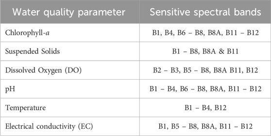
Table 3. Input variables used in Model 1 experiment.

2.3.2 Random forest regression

The Random Forest Regression (RFR) algorithm is known to be a reliable and highly predictive regressor that can deal with non-linear data (Mpakairi et al., 2023). To perform predictions, it builds a forest of various decision trees and combines them to have more accurate and stable results (Rodriguez-Galiano et al., 2012). The randomness of the RFR is introduced by randomly selecting samples and predictors from the dataset set to build each decision tree (Xu et al., 2021). By resampling the input dataset using bootstrapping, i.e., generating multiple training (i.e., 65% of the dataset) and testing sets (35% of the dataset), RFR builds multiple decision trees and makes the final predictions using the average of predictions across the trees (Xu et al., 2021). Additionally, this algorithm requires calibration based on a set of hyperparameters, which include the number of trees, maximum tree depth, minimum samples per leaf, minimum samples per split and the random seed. These hyperparameters influence model performance and robustness, necessitating careful calibration to optimise results (Mpakairi et al., 2023). In this study, the RFR hyperparameters for the two modelling experiments, i.e., Model 1 (Water quality sensitive spectral bands only) and Model 2 (spectral bands + indices), were tuned using repeated k-fold cross-validation (3-fold, repeated 3 times) to enhance the model’s stability and reliability. Hyperparameter tuning was performed using a tune Length of 5, which enables automatic selection of the best combination of hyperparameters within the Caret R Package (Probst et al., 2018).

The Normalized Difference Chlorophyll Index (NDCI), the Red-Green Index (RGI), the Fluorescence Line Height (FLH), the Normalized Difference Vegetation Index (NDVI), and the Maximum Chlorophyll Index (MCI), which have been found to enhance the detection of spatio-temporal patterns of the six water quality parameters were used in this study (Lu et al., 2016; Pawlik et al., 2024; Rawat and Singh, 2024; Salls et al., 2024). Table 4 shows the five spectral indices with their formulas.

Table 4

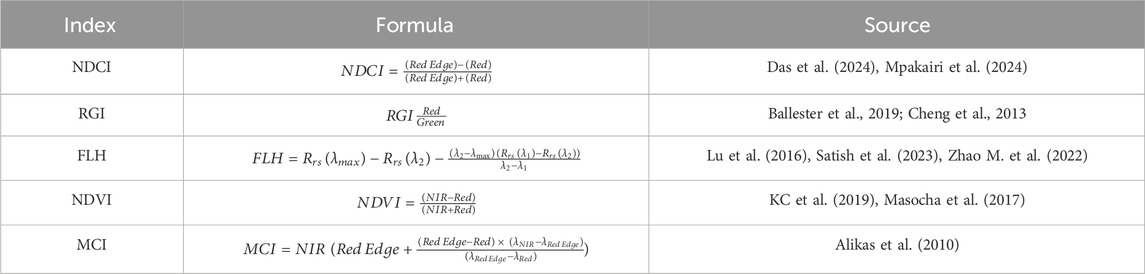
Table 4. Spectral indices computed from Sentinel-2 images.

The RFR model developed for this study also provided the variable importance scores, which aid in understanding the influence of various inputs (i.e., spectral bands + indices) on the predictions. Based on the accuracy assessment using R² and RMSE, the most accurate RFR model for each WQ parameter was applied to the land-masked Sentinel-2 images to generate spatial predictions of the WQ parameter.

2.3.3 Accuracy assessment

The performance of the models was evaluated using the coefficient of determination (R², Equation 1) and the root-mean-square error (RMSE, Equation 2). The R² assesses the agreement or disagreement between observed and predicted values, thus providing insights into the proportion of variance explained by the model and model accuracy (Chicco et al., 2021). In contrast, the RMSE quantifies the error between observed and predicted values, thus providing insights into the model precision (Chicco et al., 2021). These metrics are widely used in regression analysis and model evaluation (Richter et al., 2012; Tian et al., 2023; Zhao Y. et al., 2022).

$R^2=1-\frac{{\displaystyle {\sum }_{i=1}^n}{\left(Y_i-{\widehat{Y}}_i\right)}^2}{{\displaystyle {\sum }_{i=1}^n}{\left(Y_i-{\overline{Y}}_i\right)}^2}(1)$

$RMSE=\sqrt{\frac{{\displaystyle {\sum }_{i=1}^n}{\left(Y_i-\overline{Y}\right)}^2}{n}}(2)$

where: ${\mathrm{Y}}_{\mathrm{i}}$ represents the observed values, ${\mathrm{Ŷ}}_{\mathrm{i}}$ represents the predicted values, $\overline{\mathrm{Y}}$ is the mean of observed values, and $n$ is the total number of observations.

3 Results

3.1 Performance of various experimental models for predicting WQ parameters

The performance of the Random Forest Regression (RFR) water quality prediction models was assessed using R² and RMSE based on 35% out-of-the-bag (OOB) samples. The experiments were designed using different model configurations, i.e., Model 1 – consisting of sensitive Sentinel-2 spectral bands to water quality parameters and Model 2 – consisting of all Sentinel-2 spectral bands and carefully selected spectral indices. The results for optically active water quality parameters are presented in Figure 2. In Figures 2a–c, it is shown that chlorophyll-a was poorly predicted under high-flow (i.e., wet) conditions than under low-flow (i.e., dry) conditions. Models built for both flow conditions underestimated chlorophyll-a values, with the greatest underestimation occurring under high-flow conditions. Among the high-flow models, Model 2 (B1-B8, B8A, B11-B12 + (NDCI, RGI, FLH, NDVI and MCI), Figures 2a,c) had better performance, with 9% better R² value and lower RMSE by 2.89 μg/L when compared to Model 1 (consisting of sensitive bands only). In contrast, Model 1 achieved a marginally better R² and RMSE by 1% and 0.06 μg/L, respectively, under low-flow conditions (Figures 2b,d).

Figure 2

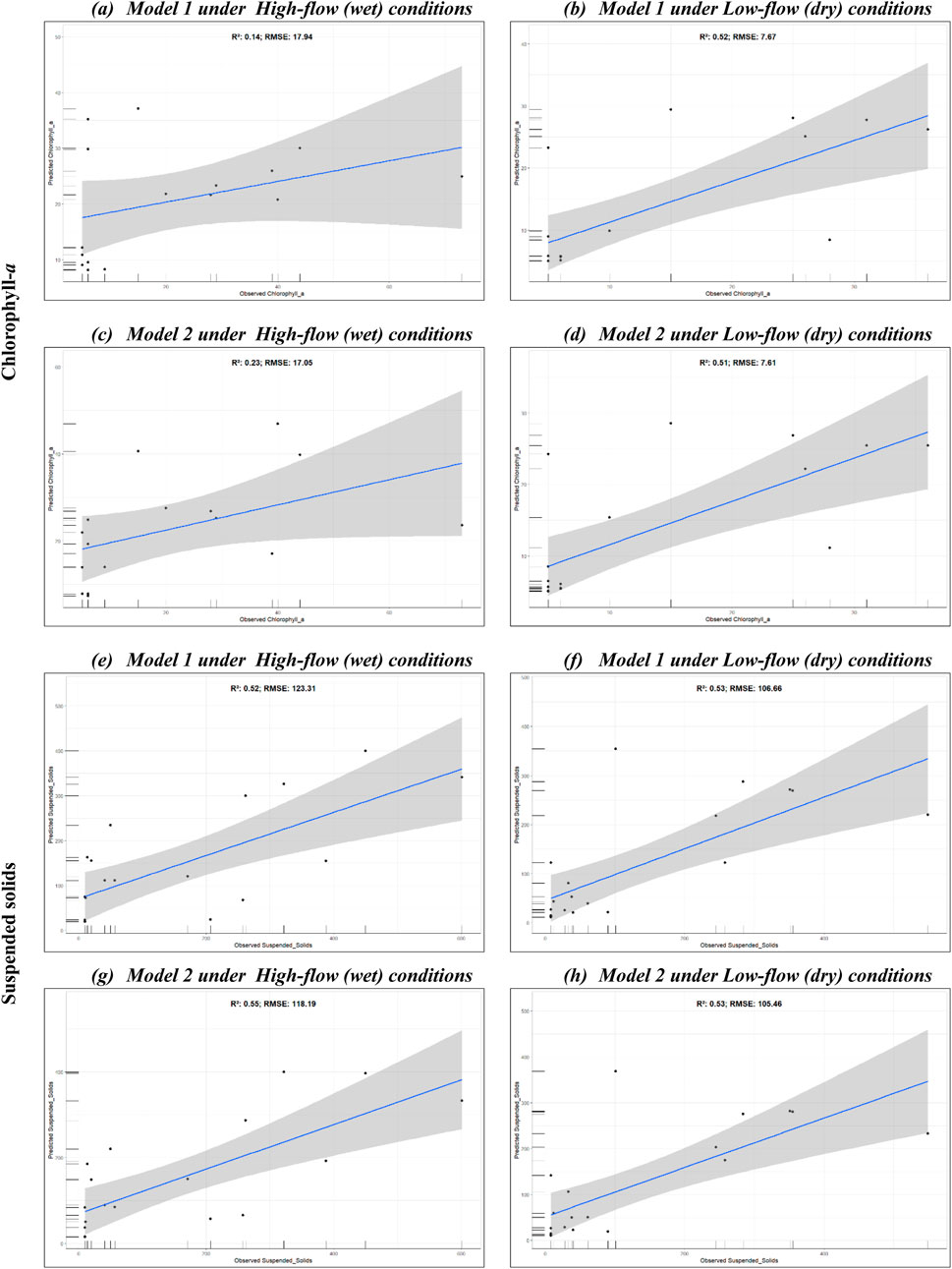
Figure 2. Random Forest Regression (RFR) models for optically active water quality parameters. (a–d) show scatterplots for chlorophyll-a, while (e–h) show plots for suspended solids.

Like chlorophyll-a models, suspended solids models (Figures 2e–h) underestimated suspended solids concentrations; however, the accuracy (R²) did not vary markedly between high-flow (wet) and low-flow (dry) conditions. Model 2 (consisting of spectral bands + indices, Figure 2g) performed slightly better, i.e., by 3% and ΔRMSE of 5.12 mg/L, while the low-flow models had equivalent R²; however, the RMSE for Model 2 was marginally lower, i.e., by 1.2 mg/L.

The prediction accuracy results for non-optically active water quality parameters (i.e., DO, pH, Temperature, and EC) are presented in Figure 3. Both RFR models, i.e., Model 1 (consisting of sensitive Sentinel-2 spectral bands to water quality parameters) and Model 2 (consisting of spectral bands + indices), indicated a high degree of accuracy, i.e., R² $\ge$ 75% in predicting DO concentrations under high-flow (wet) and low-flow (dry) conditions (see Figures 3a–d). However, under high-flow (wet) conditions, Model 1 emerged as the optimal model for DO prediction with a 2% higher R² value and 0.05 mg/L lower RMSE as compared to Model 2. Under low-flow (dry) conditions, Model 2 emerged as the optimal model for predicting DO concentrations, with a 1% better R² value and 0.09 mg/L lower RMSE as compared to Model 1. However, as shown, the differences were marginal. Similarly, these models also had good accuracies in predicting EC (see Figures 3m–p), where models under low-flow (dry) conditions had relatively higher R² > 60%, while models under high-flow (wet) conditions had R² < 0.55. Under low-flow (dry) conditions, Model 1, under high-flow conditions was also more accurate, exhibiting better R², i.e., by 8%, and 23.84 μs/cm lower RMSE relative to Model 2.

Figure 3

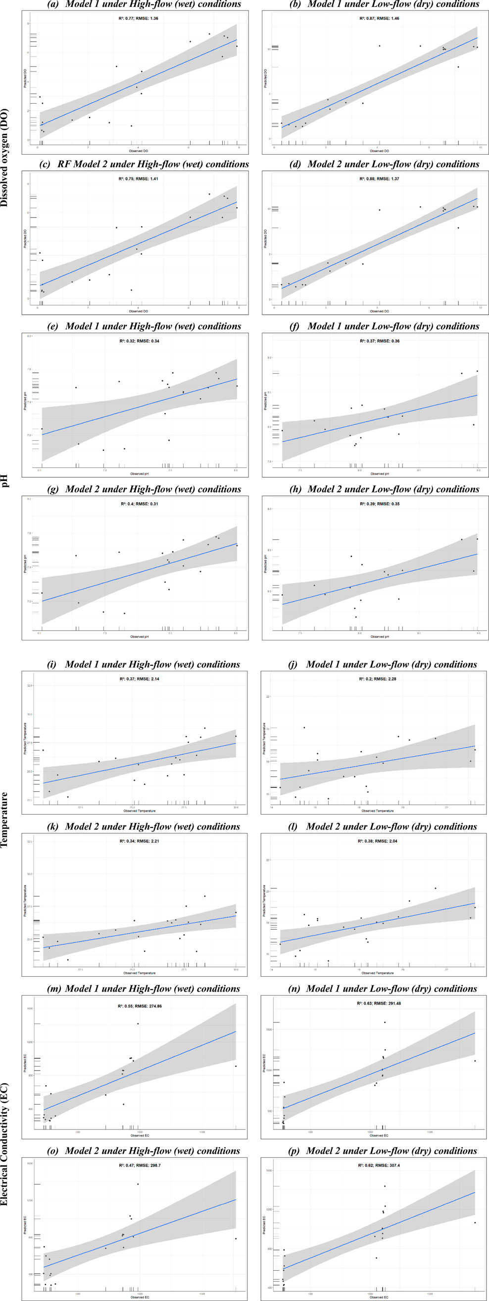
Figure 3. Random Forest Regression (RFR) models for non-optically active water quality parameters. (a–d) show scatterplots for Dissolved Oxygen (DO), (e–h) are for pH, (i–l) are for Temperature, and (m–p) for Electrical Conductivity (EC).

The pH and Temperature models exhibited relatively low accuracy (i.e., R² $\le$ 40%). For pH (see Figures 3e–h), Model 2 resulted in better performance under both high-flow (wet) and low-flow (dry) conditions, where R² values were better by 8% and 2%, respectively, and RMSE values were lower by 0.03 and 0.01, respectively. While the difference in R² between Model 1 and Model 2 under high-flow conditions can be considered marked, the difference between model accuracies under low-flow conditions was rather marginal. Water Temperature (see Figures 3i–l) was better predicted by Model 1 under high-flow conditions, i.e., ΔR² of 3% and ΔRMSE of 0.07°C, while Model 2 had better prediction accuracy under low-flow conditions, i.e., ΔR² of 18% and ΔRMSE of 0.24°C.

3.2 Variable importance of various experimental models

The Random Forest algorithm provides global variable importance using a Percentage Increase in Mean Squared Error (%Increase in MSE) which is a key feature for interpreting predictions and identifying the most influential variables contributing to model performance (Simon et al., 2023). A study by Li and Zha (2019), used this approach to assess the importance of each predictor by measuring how much the model’s error increased when each variable was randomly permuted multiple times. An increase in prediction error showed that the variable was important for accurate prediction when its permuted. Thus, a larger % of Increase in MSE indicates a stronger importance of each predictor variable (Kaveh et al., 2023). Similarly, in this study, the % Increase in MSE approach was used to identify the most influential Sentinel-2 bands and spectral indices for water quality parameter predictions under different modelling scenarios and flow conditions (i.e., high-flow vs. low-flow). Figure 4 presents the results for optically active water quality parameters. Indeed, the number of variables displayed for each modelling scenario (i.e., Model 1- sensitive spectral bands vs. Model 2 - spectral bands + indices) are different due to the configuration of each scenario. Overall, the influential variables vary by flow conditions (or season) and certainly by modelling scenario. Under high-flow (wet) conditions (Figure 4c), B8 (NIR) had the highest influence on the Model 1 prediction accuracy (i.e., %Increase in MSE % $\cong$ 9%), followed by B4 (Red) and B12 (SWIR2). The least contributing spectral band was B1 (Coastal aerosol band). Interestingly, these influential spectral bands in Model 1 were also featured in the top five most important variables in Model 2, while B1 was featured in the top five least important variables with a %Increase in MSE <3%, thus revealing some level of consistency. The Red-Green Index (RGI) was the top most influential variable (%Increase in MSE >8%). Variables known to be sensitive to Chlorophyll-a, such as B8A (NIR2), NDVI, B6 (Red-edge 2), B7 (Red-edge 3), and Fluorescence Line Height (FLH) index, were ranked in the middle, showing their intermediate importance in Model 2.

Figure 4

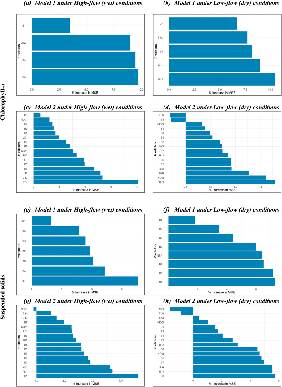
Figure 4. Random Forest variable importance showing influential variables for estimating (a–d) chlorophyll-a and (e–h) suspended solids under different model configurations and flow conditions, i.e., high-flow (wet season) and low-flow (dry season).

Under low-flow (dry) conditions (Figures 4b,c), SWIR bands (B11 and B12), red-edge band (B6) and narrow NIR band (B8A) showed most influence to Model 1 predictions with >7.5 %Increase in MSE <11%. Whereas B7’s (red-edge 3) variable importance exceeded 5%, it was the lowest. Comparatively, B12 (SWIR2) was the top most influential variable to Model 2 under the same flow-conditions (i.e., low-flow), while the other important bands to Model 1 were not in the top five most or least important variables of Model 2 importance results, thus had rather intermediate importance, albeit their relatively low %Increase in MSE, i.e., $\ge$ 3%. Interestingly, FLH and B3 (Green) negatively contributed to Model 2 predictions.

Figures 4e–h show that, under high-flow (wet) conditions, both modelling scenarios’ (i.e., Model 1 and Model 2) performance was highly influenced by B1 (Coastal aerosol), with %Increase in MSE ∼10% and >8%, respectively. Other important variables to Model 1’s performance included B4, B6, and B2, while B3, B5 and B11 contributed the least to the prediction accuracy of suspended solids. However, B11 had the lowest variable importance, which is also consistent with Model 2 variable importance results for the high-flow conditions. B3 and B5 were neither in the top five most or least important variables, showing that although their influence was relatively low, they also contributed positively to Model 2 predictions. In contrast, the Normalized Difference Chlorophyll Index (NDCI) understandably contributed negatively to Model 2 performance because it is a Chlorophyll-specific index. Under low-flow conditions, B8 (NIR) had the highest variable importance for both Model 1 (>6) and Model 2 (<5). B2 (visible spectrum) contributed the least ($\cong$ 2) to Model 1 performance, while the MCI and FLH had negative values for variable importance in Model 2. The variable importance results for the RFR models of non-optically active water quality parameters are presented in Figure 5. Similar to the importance results for optically active parameters, results here also varied by modelling scenario and flow conditions (or season). Under high-flow conditions, all (sensitive) spectral bands were highly influential to Model 1 predictions, but B8A, B7 and B6 were the topmost important variables, while B11 and B2 were the least important in predicting DO (Figure 5a).

Figure 5

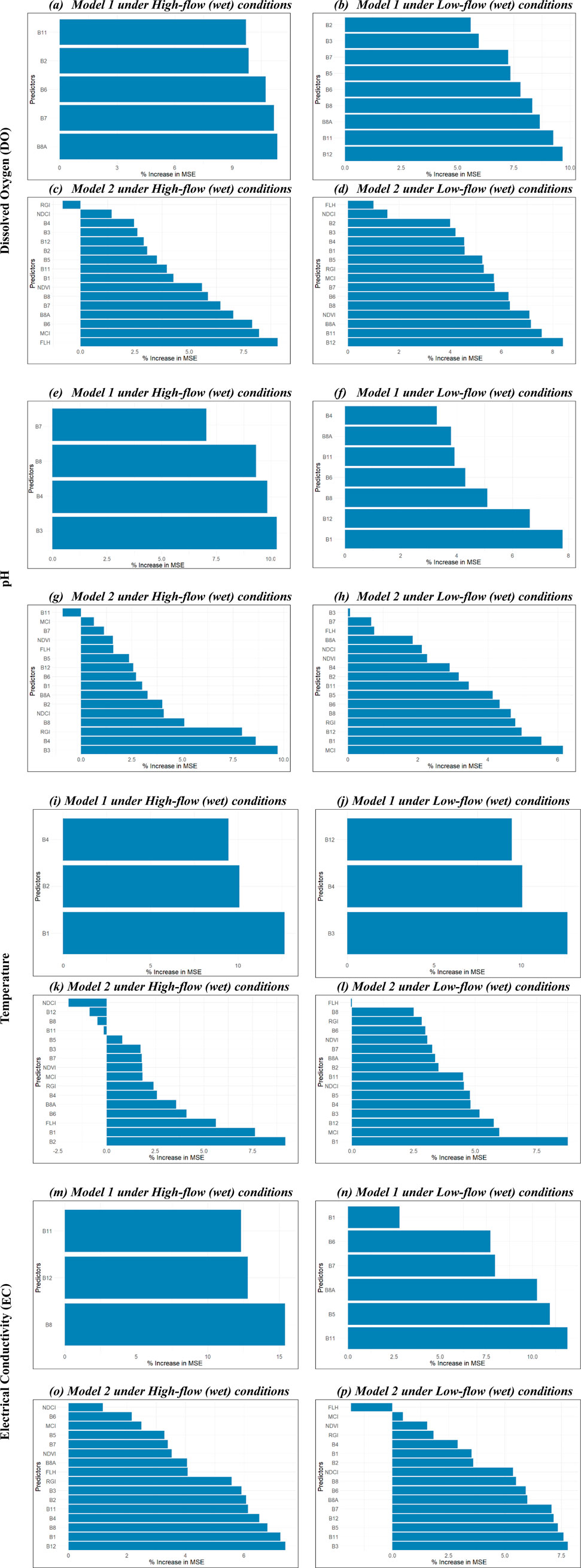
Figure 5. Random Forest variable importance showing influential variables for estimating (a–d) DO, (e–h) pH, (i–l) Temperature, and (m–p) EC, under different model configurations and flow conditions, i.e., high-flow (wet season) and low-flow (dry).

Under low-flow (dry) conditions, SWIR (B11 and B12), NIR bands (B8 and B8A) and red-edge band (B6) were the top five most important variables influencing Model 1 performance in predicting DO (Figure 5b). On the other hand, variables such as B2 and B3 were among the least influential. Similar to Model 1 under high-flow conditions, B6, B7 and B8A featured in the top five most important variables in Model 2 alongside MCI and FLH, which had the highest %Increase in MSE (Figure 5c). RGI contributed negatively to the model performance, while NDCI, B4, B3, and B12 were among the top five least important variables in predicting DO. When the RFR model was run with spectral bands + indices (i.e., Model 2) under low-flow (dry) conditions (Figure 5d), important variables also matched those in Model 1 under the same conditions. For example, B11, B12 and B8A were the top most influential variables, while B2 and B3 were among the top five least important variables, alongside indices such as FLH and NDCI. Important variables for predicting pH using RFR under different modelling scenarios (Figures 5e–h) reveal that under high-flow conditions, B3, B4 and B8 were the most influential variables to Model 1 performance, while B7 was the least (Figure 5e). This was also consistent with Model 2 under the same flow conditions (i.e., season), where they featured in the top five most influential variables, along with RGI and NDCI (Figure 5g). A similar pattern can be observed under low-flow (dry) conditions, where B1, B12, B8 and B6 were most influential in both modelling scenarios, but RGI and MCI were also part of Model 2’s most important variables (Figures 5f,h).

B1 and B2, which were influential to Model 1 water Temperature predictions under high-flow conditions (Figure 5i), also featured as the top-most influential variables in Model 2 (Figure 5k) under the same conditions. However, NDCI, B12, B8, and B11 had a negative influence on Model 2 predictions. Similarly, sensitive spectral bands used in Model 1 under low-flow conditions all featured in the top five most important variables in Model 2, along with MCI (Figures 5j,l). FLH had a negative influence on Model 2’s performance (Figure 5l). Finally, Figures 5m–p show important variables for predicting Electrical conductivity (EC). As shown, important variables from Model 1 and Model 2 are consistent. For example, all variables used in Model 1, i.e., B11, B12, and B8, were featured in the top five most important variables for Model 2 under high-flow conditions (Figures 5m,o). Also, B8A, B5, and B11, identified as most important for Model 1 predictions under low-flow conditions, were among the top influential variables for Model 2 (Figures 5n,p). FLH contributed negatively to the Model 2 performance under low-flow conditions.

3.3 Spatio-temporal patterns of water quality parameters

The models which resulted in the best accuracy, were used to predict the spatio-temporal patterns of WQ parameters in the study area. Table 5 summarises the prediction results, the best models (in bold) and important variables.

Table 5

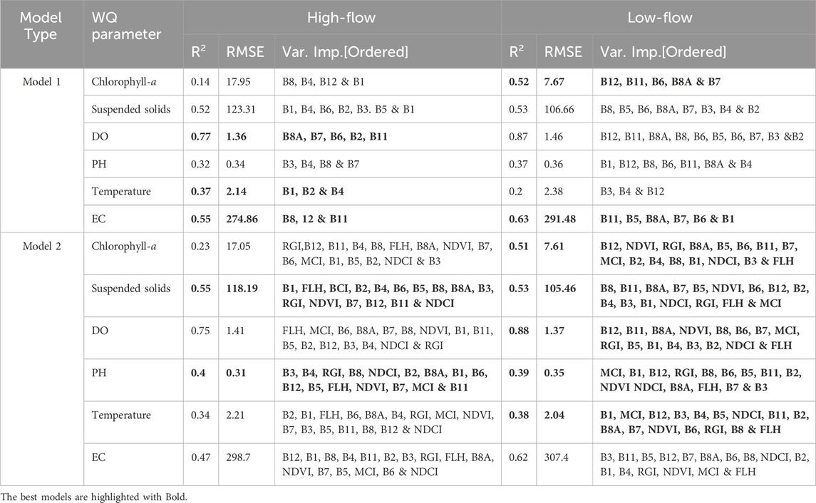
Table 5. Summary of prediction accuracy assessment.

Two models were used to illustrate chlorophyll-a concentrations in Cradlemoon Lake under high-flow and low-flow conditions (Figure 6), based on differences in model accuracy. As predicted by Model 2, the maximum value of chlorophyll-a was 15.6 μg/L in the high-flow conditions, and as predicted by Model 1 (which had higher accuracy results), the maximum value was 5.36 μg/L in the low-flow conditions. Furthermore, the study results also showed significant temporal variations in the minimum values of chlorophyll-a as the lowest value of chlorophyll-a was 13.75 μg/L under high-flow conditions and 5.16 μg/L under low-flow conditions. During the high-flow conditions, Model 2 predicted that chlorophyll-a was concentrated across the water body and its lower values were found on the tributary of the water body. Model 1, in the low-flow conditions, demonstrated higher accuracy and predicted that maximum chlorophyll-a was also concentrated in the centre of the lake; however, some areas within the centre exhibited lower chlorophyll-a concentrations.

Figure 6

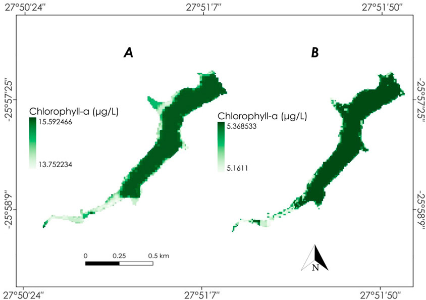
Figure 6. Chlorophyll-a spatio-temporal patterns estimated by Model 2 for the high-flow (A) conditions and Model 1 for the low-flow (B) conditions. The colour scales in (A,B) differ to better highlight the spatial distribution of chlorophyll-a concentrations observed under different flow conditions.

The spatio-temporal coverage of suspended solids was predicted using Model 2 (Figure 7) for both the high-flow and low-flow conditions. The results of the model predicted suspended solids maximum values at 118.34 mg/L for the high-flow conditions, while low-flow condition values were decreased to 93.7 mg/L. The lowest suspended solids values were predicted in low-flow conditions at 46.96 mg/L, while the high-flow condition minimum values were predicted to be 90.80 mg/L. In both flow conditions, high suspended solids values were more concentrated in the banks and the tributary (Crocodile River) of the Cradlemoon Lake. The difference was more pronounced in terms of concentration, with higher suspended solids levels observed during high-flow conditions and decreased during low-flow conditions.

Figure 7

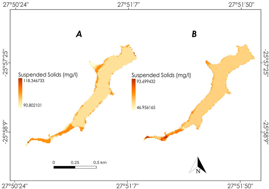
Figure 7. Suspended solids spatio-temporal patterns estimated by Model 2 for the high-flow (A) and low-flow (B) conditions. The colour scales in (A,B) differ to better highlight the spatial distribution of chlorophyll-a concentrations observed under different flow conditions.

Model 1 showed the highest accuracy for DO concentrations under high-flow conditions, whereas Model 2 performed best under low-flow conditions. As seen in Figure 8, the predicted concentration of DO under low-flow conditions ranged between 3.75 mg/L and 4.32 mg/L. In contrast, under high-flow conditions, DO concentrations ranged between 2.09 mg/L and 2.84 mg/L. Regarding spatio-temporal patterns, the distribution of DO values differed between the two conditions. During high-flow conditions, higher DO values were mainly concentrated along the edges of Cradlemoon Lake, whereas under low-flow conditions, high DO values were spread across the centre of the lake, with lower values near the edges.

Figure 8

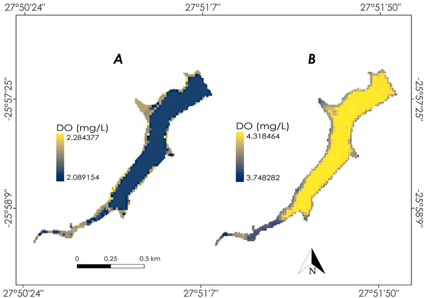
Figure 8. DO spatio-temporal patterns estimated by Model 1 for the high-flow (A) conditions and Model 2 for the low-flow (B) conditions. The colour scales in (A,B) differ to better highlight the spatial distribution of chlorophyll-a concentrations observed under different flow conditions.

Regarding pH spatio-temporal patterns, Model 2 performed better in predicting pH levels under both high-flow and low-flow conditions compared to Model 1, which had lower accuracy. The model showed only small differences between the two flow conditions, with the highest pH reaching 8.01 under high-flow conditions and 7.76 under low-flow conditions. The lowest pH levels were also similar, at 7.97 during low-flow and 7.63 during high-flow. Figure 9 shows the spatio-temporal patterns of pH, where the lowest levels were predicted along the northern edges of Cradlemoon Lake and the southern edges of its southern tributary, the Crocodile River. Under low-flow conditions, pH levels were slightly higher overall, meaning fewer areas exhibited lower pH values—lower pH was mainly predicted along the lake’s tributary.

Figure 9

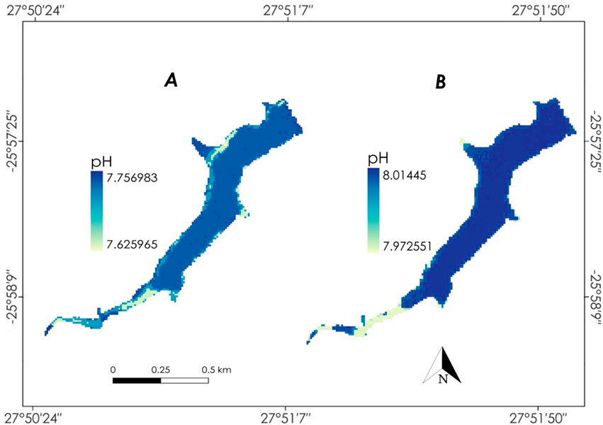
Figure 9. pH spatio-temporal patterns estimated by Model 2 for the high-flow (A) and low-flow. The colour scales in (A,B) differ to better highlight the spatial distribution of chlorophyll-a concentrations observed under different flow conditions.

Temperature predictions for Cradlemoon Lake (Figure 10) used Model 1 for high-flow conditions and Model 2 for low-flow conditions. Results from Model 1 during high-flow conditions predicted Temperatures ranging between 25.85°C and 25.83°C, with a relatively uniform distribution across the lake, except for slight variations along the edges. Although Model 1 performed better than Model 2 in terms of accuracy metrics, the overall accuracy remained low. In contrast, Model 2 predictions for low-flow conditions indicated significantly lower Temperature, ranging between 17.80°C and 17.45°C, with higher Temperature concentrations along the lake’s edges and inflow zones.

Figure 10

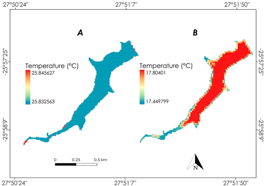
Figure 10. Temperature spatio-temporal patterns estimated by Model 1 for the high-flow (A) conditions and Model 2 for the low-flow (B) conditions. The colour scales in (A,B) differ to better highlight the spatial distribution of chlorophyll-a concentrations observed under different flow conditions.

The prediction of EC spatio-temporal patterns (Figure 11) for Cradlemoon Lake was conducted using Model 1 of the two random forest models. During high-flow conditions, model predictions revealed that EC values ranged from 259.18 µS/cm to 454.01 µS/cm, with lower concentrations distributed across most of the lake and higher values concentrated along the edges, particularly near inflow zones such as the Crocodile River, a tributary of the lake. This pattern suggests that increased water inflow dilutes dissolved ions, reducing overall EC levels compared to low-flow conditions. In contrast, under low-flow conditions, EC values were higher, ranging from 387.86 µS/cm to 643.39 µS/cm, with the highest concentrations near the lake edges and inflow zones.

Figure 11

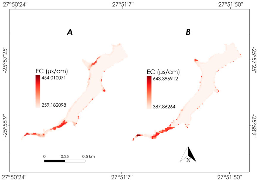
Figure 11. EC spatio-temporal patterns estimated by Model 1 for the high-flow (A) and low-flow (B) conditions. The colour scales in (A,B) differ to better highlight the spatial distribution of chlorophyll-a concentrations observed under different flow conditions.

4 Discussions

4.1 Performance of RFR in estimating water quality parameters under high-flow (i.e., wet) and low-flow (i.e., dry) conditions

Worsening water quality in sub-Saharan Africa requires integrated water resources management incorporating satellite technology and machine learning algorithms to provide relevant information about the changes in water quality on important lakes and dams. Previous studies focused on large lakes and dams, while smaller water bodies are neglected. This study aimed to evaluate the predictive performance of the Random Forest Regressor (RFR) in estimating both optically active and non-optically active water quality parameters under high-flow (wet) and low-flow (dry) conditions in small water bodies within the COHWHS. Two RFR models were developed with Model 1, including only the Sentinel-2 bands identified as sensitive to specific water quality parameters in our previous work (Ngamile et al., under review) and Model 2, which incorporated all Sentinel-2 spectral bands (B1-8, B81, B11 and B12) along with five spectral indices. Among the parameters analysed, suspended solids predictions showed higher accuracy compared to chlorophyll-a across both high-flow and low-flow conditions and for both Model 1 and Model 2. However, Model 2 demonstrated greater accuracy, likely due to incorporating additional spectral bands and indices, which enhanced the model’s ability to capture the spectral variability associated with suspended solids.

For high-flow conditions, Model 2 achieved an R² of 0.55 and a Root Mean Square Error (RMSE) of 118.19 mg/L, while for low-flow conditions, the model yielded an R² of 0.53 and an RMSE of 105.46 mg/L. Previous studies (Kupssinskü et al., 2020; Saberioon et al., 2020) have shown significantly higher accuracy results (R² > 0.8 and low RMSE) for suspended solids predictions using the random forest model and Sentinel-2 MSI data. However, in our study, the results were lower (relative to previous studies) despite the use of the same approach. This can be attributed to how high turbidity (caused by elevated suspended solids) leads to reflectance saturation, which reduces the sensitivity of certain spectral bands for monitoring suspended solids, ultimately lowering model accuracy (Doxaran et al., 2002). Jiang et al. (2023) highlighted that turbid water events significantly affect suspended solids estimation. Turbidity is caused by suspended organic and inorganic particles, such as mud and fine sand, which increase water cloudiness (Azis et al., 2015). Under high-flow conditions, increased runoff likely introduced more suspended solids, leading to higher turbidity levels, which in turn masked the spectral signal of suspended solids, lowering model accuracy. Despite the high performance in suspended solids estimation, for Model 2, variable importance results revealed B1 (coastal aerosol) and B8 (NIR) as having the highest variable importance under high-flow and low-flow conditions, respectively. Previous studies (Caballero et al., 2018; Liu et al., 2017; Pasaribu et al., 2024) have demonstrated the effectiveness of NIR in estimating suspended solids concentrations, aligning with our study results.

For instance, Liu and Zhao (2017) highlighted the utilisation of Sentinel-2 NIR (B8-B8A) in analysing turbidity levels (in the Poyang Lake, China), which directly correlate with the concentration of suspended solids in water bodies. This was further supported by Molner et al. (2023), who revealed that the Sentinel-2 NIR bands provided valuable information on measuring suspended solids in the Albufera Lagoon (Spain). On the other hand, chlorophyll-a model predictions were affected by the dominance of suspended solids under high-flow conditions, causing chlorophyll-a spectral signatures to be weak. As a result, Model 1’s prediction of chlorophyll-a in high-flow conditions had an R² of 0.14 and RMSE of 17.94, while Model 2 performed slightly better, with an R² of 0.23 and an RMSE of 17.05. These low chlorophyll-a prediction results demonstrate how increased suspended solids often have a stronger spectral signal than chlorophyll-a, particularly in turbid waters (Liu et al., 2023). Anthropogenic activities (such as mining) around the COHWHS contribute to increased transportation of suspended solids, and elevated suspended solids lead to increased turbidity (Azis et al., 2015; Durand et al., 2010). The reported R² values for chlorophyll-a model predictions indicate low model performance, which is expected due to spectral challenges, as turbidity interferes with its estimation (Cheng et al., 2013). In contrast, chlorophyll-a predictions under low-flow conditions showed moderate accuracy (as seen in Figures 2b,d), likely due to a reduction in suspended solids and turbidity. A variable importance ranking was conducted to identify key input bands and spectral indices influencing chlorophyll-a predictions using the low-flow Model 1 and Model 2. The results showed that B12 was the most consistent and influential predictor, differing from previous studies (Arora et al., 2022; Llodrà-Llabrés et al., 2023), which have emphasised the green (B3) and RE bands (B5- B7) for chlorophyll-a estimation.

The NDVI spectral index also demonstrated how the NIR bands (B8 and B8A) and B4 (red) can be used to predict chlorophyll-a as it closely followed B12’s high variable importance results (Model 2) under low-flow conditions. This index has been used in various studies (Lekhak et al., 2023; Meng et al., 2024; Nikoo et al., 2024) concerning chlorophyll-a estimation. Moreover, Model 2 demonstrated the RGI as having a high variable importance in chlorophyll-a estimation under high-flow conditions. It has been used by Cheng et al. (2013) who estimated chlorophyll-a in turbid waters of the Taihu Lake, China, and it is a measure of the ratio between the reflectance in the Red band and the Green band (Motohka et al., 2010). This shows the red band (B4) can also be used for chlorophyll-a estimation as supported by other studies such as Zheng and DiGiacomo (2017). Under low-flow conditions, Model 2 showed a negative effect on chlorophyll-a prediction when incorporating Band 3 (B3) and the FLH spectral index. This could be attributed to their poor correlation with chlorophyll-a since it had low concentrations in low-flow conditions. B3 (Green, 560 nm) typically has weaker sensitivity to chlorophyll-a compared to red (B4) and near-infrared (B8) bands, making it less effective in prediction (Ha et al., 2017). Similarly, the FLH index, which estimates chlorophyll fluorescence, may not perform well under low-flow conditions because of changes in optical properties and light absorption which may be caused by other water quality factors such as suspended solids and turbidity (Kowalczuk et al., 2019). As a result, these features might introduce noise, reducing the model’s predictive accuracy for chlorophyll-a.

For non-optically active water quality parameters, both RFR models performed well in retrieving DO and EC during low-flow conditions. For DO predictions, Model 1 and Model 2 had R² values of 0.87 and 0.88, respectively, while the RMSE values were 1.46 and 1.37, respectively. Among all the parameters (both optical and non-optical), DO had the highest prediction accuracy, likely due to its strong relationships with chlorophyll-a, suspended solids, and Temperature. For instance, increased chlorophyll-a increases phytoplankton, which can lead to higher oxygen production through photosynthesis (Kunlasak et al., 2013). However, elevated suspended solids - especially those influenced by sewage and related sludge (as experienced in our study area) - can counteract this by reducing light penetration (suspended solids block sunlight, limiting photosynthesis and, in turn, oxygen production (Bilotta and Brazier, 2008; Perivolioti et al., 2024)). Moreover, water with suspended solids retains heat, further increasing Temperature levels and high Temperatures in water generally lead to less dissolved oxygen, affecting aquatic life (Koue, 2024; Paaijmans et al., 2008). Conversely, when suspended solids decrease, chlorophyll-a levels tend to increase, promoting more photosynthetic oxygen production, which can lead to an increase in DO. These are the activities which were observed in our study where DO concentrations were higher during the low-flow conditions due to lower Temperatures and reduced suspended solid levels, and slightly increased photosynthetic activities. All these factors likely contributed to higher model accuracy since DO shows predictable seasonal and spatial trends and has strong relationships with suspended solids, chlorophyll-a and Temperature.

Furthermore, our study found that the SWIR bands (B11-B12) and NIR band (8A) showed consistency in the variable importance sequence under low-flow conditions, which had higher model accuracy with both Model 1 and Model 2. This was further attributed to DO’s strong relationship with suspended solids, a water quality parameter that has been estimated with NIR and SWIR bands (Caballero et al., 2018). As Figure 5d illustrates, these results on variable importance ranking were further followed by B8 (NIR), the NDVI and RE bands that are known for their prediction of chlorophyll-a. The novelty of our study further lies in how spectral indices have been used to enhance water quality parameter estimation, particularly when using Model 2 and this is demonstrated where the FLH index - which is known for chlorophyll-a estimation - had the highest variable importance in estimating DO under high-flow conditions. All these results demonstrate the high performance of indirect DO estimation in our study. EC had the second-highest prediction accuracy among the parameters under low-flow conditions, with R² values exceeding 0.6 in both Model 1 and Model 2. This can be attributed to reduced surface run-off under these conditions (low-flow, i.e., dry conditions), causing less dilution of dissolved salts and ions (which EC measures), which remain more stable and concentrated (Kumar Roy et al., 2015). This activity can make it easier for remote sensing models to detect patterns. There is a complex relationship between suspended solids, dissolved ions, salinity, and EC. Suspended solids can dilute salts and ions, which influence salinity and EC (Zezulka et al., 2024).

Under low-flow conditions, when suspended solids are low, the concentration of dissolved ions may increase, leading to higher EC. Thus, EC can be indirectly estimated using suspended solids and salinity as optically active water quality indicators. For instance, Bouaziz et al. (2018) found that EC is correlated with salinity while Li J.et al. (2023) demonstrated that the SWIR bands were more sensitive to soil salinity (which can be applied to salinity in water) and these results align with the results of our study where B11 (SWIR) showed a strong relationship with EC. This is further supported by Ndou (2023) who also used Sentinel-2 to predict various non-optically active water quality parameters on the South African Setumo dam and found that B11 was highly sensitive to EC variations. Temperature and pH had the lowest model performance results (R² < 0.5) for both the high-flow and the low-flow conditions. For Temperature, several studies (Ellis et al., 2024; Murphy et al., 2021; Vanhellemont, 2020) have used thermal bands of satellite sensors such as the Thermal InfraRed Sensor (TIRS) on board Landsat-8 to predict water surface Temperature. Other studies, such as the Medina-Lopez and Ureña-Fuentes (2019), estimated sea surface temperature (SST) using Sentinel-2 Level 1-C Top of Atmosphere (TOA) reflectance data, achieving a correlation coefficient of 84% and a mean error of 0.4°C. Similarly, Dyba et al. (2022) used Landsat-8 imagery to estimate lake surface water temperature in Poland, comparing linear regression, random forest, and the Landsat Level-2 Surface Temperature Science Product (LST-L2). Their results showed that the RFR model performed best (R² = 0.89, RMSE = 1.83°C). However, in this study, different results were observed. Sentinel-2, which lacks thermal sensors, and the random forest models performed poorly in Temperature estimation despite the inclusion of other input variables, i.e., spectral water indices.

Mohammadpour et al. (2022) have emphasised that random forest models work well when strong predictive relationships exist between independent variables (Sentinel-2 bands) and the dependent variable (Temperature), and in this study, Temperature had a poor correlation with the Sentinel-2 bands. Despite the absence of thermal sensors, Model 1 (high-flow) and Model 2 (low-flow) identified the coastal aerosol Band 1 (B1) as the most important variable in Temperature prediction. The Sentinel-2 coastal aerosol band (B1) is known for coastal habitat mapping and satellite-derived bathymetry estimation (Poursanidis et al., 2019), while the random forest model is known for its ability to capture complex relationships between water quality parameters (Dewi et al., 2024). This may explain why, despite the absence of thermal sensors, B1 may have indirectly captured water quality parameter activities linked to Temperature variations, such as habitat mapping. Habitat mapping involves predicting aquatic habitats and has been affected by climate change-driven Temperature and heat variations, highlighting its connection to Temperature (Dewi et al., 2024). For pH estimations, Model 2 outperformed Model 1, particularly under the high-flow conditions. However, results remained poor, with an R² of 0.4 and an RMSE of 0.31. In contrast, Adusei et al. (2021) assessed pH on the Owabi reservoir using Sentinel-2 (and Landsat-8), with results revealing an R² of 0.95 and RMSE of 0.07 with the random forest model. The study found that in situ pH measurements had little variability, leading to strong agreement between observed and predicted values for Sentinel-2 using the random forest model.

Raghul and Porchelvan (2024) highlight that remote sensing-based water quality models depend on the relationship between spectral reflectance and in situ indicators, with parameter variability posing challenges. In this study, spatial variations in sampling locations may have introduced noise, making it harder to establish a reliable pH-spectral relationship and reducing model accuracy. Despite the lower accuracy for pH, the variable importance ranking for Model 2 under low-flow conditions showed that the MCI index, which uses Sentinel-2 RE bands (B5 and B6) to measure chlorophyll-a, was the most important predictor for pH. This can be attributed to the relationship between pH and chlorophyll-a. According to, Maradhy et al. (2022), higher pH levels are associated with increased chlorophyll-a concentrations in water, indicating a strong correlation between the two parameters. This relationship can explain why the MCI as well B3-visible spectrum (under high-flow conditions, using Model 1 and Model 2) had the highest variable importance in pH estimation. Various studies (Arora et al., 2022; Cairo et al., 2020; Shaik et al., 2021) have used these variables to predict chlorophyll-a concentrations. The prediction results of these non-optically active parameters demonstrate the effectiveness of the random forest model in capturing complex relationships between water quality parameters, highlighting how indirect methods can be used to estimate non-optically active variables. The marginal performance difference between Model 1 and Model 2 suggests that selecting only the most sensitive spectral bands was beneficial for these water quality parameters. This indicates that either model can be used for spatial and temporal predictions. However, models with lower-dimensional inputs are preferred, as they reduce computational burden by limiting the number of input variables.

4.2 Spatio-temporal patterns of optically and non-optically active water quality parameters

To analyse the health of the water bodies concerning plant presence and to evaluate the seasonal and spatial distribution of water quality parameters, in situ measurements were conducted across multiple sampling points within the study area (COHWHS), including Cradlemoon Lake. These field measurements were used to capture seasonal variability in water quality parameters through Sentinel-2 MSI satellite imagery, employing two RFR models for prediction. The model with the highest accuracy was selected to map the spatio-temporal patterns of the water quality parameters. All analysed parameters exhibited spatial variability within Cradlemoon Lake during both the high-flow and low-flow conditions (Table 6). This variability was influenced by increased runoff and inflows from the Crocodile River during the high-flow condition, leading to fluctuations in water quality parameter values. Conversely, the low-flow conditions exhibited more stable and diluted conditions, likely due to reduced inflow and less sediment transport.

Table 6

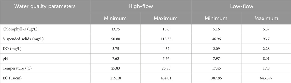
Table 6. Summary statistics of predicted water quality parameters.

Additionally, the presence of Water Hyacinth (Eichhornia crassipes) within the lake may have influenced the concentration of some parameters, such as suspended solids, leading to reduced turbidity. Water Hyacinth is an invasive species that has impacted several major South African water bodies for many years (Auchterlonie et al., 2021). Onyari et al. (2024) note that water hyacinth (E. crassipes) in freshwater ecosystems can threaten livelihoods, restrict access to clean water, and contribute to the spread of waterborne diseases. However, despite its negative impacts, several studies (De Laet et al., 2019; Eze et al., 2023; Rezania et al., 2016) highlight that, when properly managed, this plant can help reduce water pollution and improve water quality. For instance, Elizabeth et al. (2020) assessed the effectiveness of different-sized water hyacinths in filtering suspended solids and heavy metals from turbid water. Results showed that smaller plants accumulated more lead (Pb), cadmium (Cd), and copper (Cu), while roots absorbed more heavy metals than leaves and stems. Over 7 days, water hyacinths reduced total dissolved solids from 261 ppm to 204 ppm and total suspended solids from 0.0449 ppm to 0.0151 ppm. This indicates that the presence of the plant in the Cradlemoon Lake can help to control some of the pollutants that enter the water body. For this lake in particular, the water hyacinth can be found on the edges of the lake as well as on the inflow and outflow zones (the rivers such as the Crocodile River–tributary) that feed into the lake where high suspended solids values were also found.

Increased runoff during high-flow conditions contributed to increased concentrations of suspended solids and chlorophyll-a, likely due to the increased flow of sediments and nutrients from the Crocodile River and Bloubankspruit River surface and groundwater within the COHWHS is impacted by chemicals from AMD and other pollutants originating from tailing dams and abandoned mines. These issues stem from unsustainable mining practices in the West Rand. Since rivers, dams, and lakes in the area are interconnected, they influence each other, especially during high-flow conditions when increased runoff transports pollutants. In contrast, low-flow conditions produce more stable water quality, with lower concentrations of suspended solids and chlorophyll-a. This is evident in Table 6, which shows that chlorophyll-a concentrations were significantly higher during high-flow conditions, suggesting that nutrient enrichment from runoff contributes to algal growth. These trends align with findings from Jang et al. (2024), who observed that chlorophyll-a concentration increased in spring and peaked in summer (high-flow conditions), then declined before reaching a second peak in late autumn (low-flow conditions). Their study further highlights that summer rainfall introduced total suspended solids, organic matter, and nutrients (nitrogen and phosphorus) into the Namyang Reservoir, promoting active algal growth. Chlorophyll-a distribution showed minimal spatial variation between high-flow and low-flow conditions, with high concentrations consistently in the central areas of Cradlemoon Lake and lower values along the edges and inflow zones.

However, during low-flow conditions, chlorophyll-a became more prominent along the edges, likely due to reduced sediment resuspension. In contrast, high suspended solids (118.34 mg/L) during high-flow conditions were concentrated along the edges and inflow zones, likely suppressing chlorophyll-a growth. Suspended solids decreased to 93.7 mg/L in low-flow conditions but maintained a similar distribution. Suspended solids showed a clear seasonal pattern, indicating increased sediment transportation in the high-flow conditions and a decrease in the low-flow conditions due to reduced runoff and sediment deposition, a trend commonly observed in freshwater systems with distinct wet and dry seasons. Moon et al. (2024) showed similar trends where total suspended solids levels go up during the monsoon season (June–August) because heavy rain washes more sediment into the rivers. Low tide also makes total suspended solids more concentrated, while high tide spreads it. After the monsoon, with less rain and more settling, the total suspended solids start to drop. However, since the monsoon is super cloudy, satellite images do not always capture these changes well. This reduction in suspended solids and turbidity during the low-flow conditions also contributed to higher light penetration, which may have supported increased photosynthetic activity and, subsequently, higher dissolved oxygen levels. As Moon et al. (2024) and Jang et al. (2024) note that suspended solids and DO have a relationship where high total suspended solids reduce light penetration, limiting photosynthesis and lowering DO levels. It also increases oxygen consumption as organic matter decomposes, further depleting oxygen.

In the case of Cradlemoon Lake, lower suspended solids and moderate chlorophyll-a concentrations during the low-flow conditions resulted in higher DO levels, whereas higher suspended solids during the high-flow conditions led to a decline in DO, as illustrated in Table 6. The spatial distribution of DO revealed higher concentrations along the lake’s edges during high-flow conditions, while higher DO levels were concentrated toward the lake’s centre in the low-flow conditions. Moreover, DO and Temperature have an inverse relationship here; DO levels decrease as Temperature increases and vice versa (Kim et al., 2020; Li Y. et al., 2023). This trend is further emphasised by Guo et al. (2021b), who analysed Landsat and MODIS data and found that DO levels in Lake Huron declined by 6.56% between 1984 and 2019, primarily due to rising air Temperatures, among other influences. Warmer Temperatures and more sunlight can help plants and algae produce oxygen through photosynthesis, but they also make it harder for oxygen to dissolve in water and increase the activity of microbes that use up oxygen. In the same study, results found that heavy rainstorms increased nutrient runoff from farms into the lake, causing algae to grow quickly and die, leading to more oxygen being used by bacteria breaking them down. The study showed that in years when the Temperature was lower (1987 and 1992), DO was higher, but in years when it was higher (2002 and 2012), DO was lower. This suggests that rising Temperatures are a major reason for the decrease in DO, which could harm water quality in the lake. This is evident in this study of the Cradlemoon Lake as the results showed that DO values decreased when Temperature had higher ranges in the high-flow conditions and DO values increased with lower Temperature ranges in the low-flow conditions (Table 6).

This study also shows that Temperature is influenced by seasonal changes, and its predictions in the high-flow conditions did not reveal much variation, as minimum and maximum values were almost the same in terms of ranges. Under low-flow conditions, there was a slight variation in minimum and maximum values, with spatial pattern results showing the concentration of minimum values on the edges of the lake and maximum values at the centre of the lake. According to Arhin et al. (2023), the World Health Organisation (WHO) considers the acceptable pH level for drinking water to be between 6.5 and 8.5, and the pH results for this study indicate that inflow conditions had a minimal effect on overall pH balance on the Cradlemoon Lake across both the high-flow and the low-flow conditions. However, Chen and Franklin (2023) maintain that when oxygen levels are low, some microorganisms use anaerobic respiration, which can produce acidic substances like hydrogen sulphide. This makes the water more acidic, lowering the pH. This shows an existing relationship between DO concentrations and pH levels as model predictions for this study on the Cradlemoon Lake revealed that the highest maximum pH levels were recorded in the high-flow conditions, and the lowest maximum levels were recorded in the low-flow conditions when DO was also low. Regarding spatial patterns, lower pH values were revealed along the lake’s northern edges and tributary zones, suggesting localised influences from inflowing water sources. The stability of pH is consistent with findings in similar lake systems, where natural buffering capacity prevents large fluctuations despite seasonal changes in nutrient input and biological activity.

According to Gapparov and Isakova (2023), the conductivity in pure and fresh-water bodies is generally low because they contain almost no ions, yet seawater bodies generally have much higher conductivity. Polluted water bodies, however, can contain dissolved substances, chemicals, and minerals which cause an increase in dissolved ions (Rusydi, 2018). EC can, therefore, assist in measuring the concentration of dissolved ions in polluted inland water bodies. For instance, El-Zeiny et al. (2019) used Landsat OLI images to analyse EC in Qaroun Lake (>10 km²). Their results showed that EC is lowest in the east (near El-Bats drain) and increases westward due to evaporation and wastewater discharge. Under high-flow conditions, freshwater inflow lowers EC in the east, but salinity rises as water moves west. In low-flow conditions, evaporation dominates, leading to higher EC across the lake. In this study, EC followed a similar pattern with Sentinel-2 results, with lower values in the high-flow conditions and higher values in the low-flow conditions, as illustrated in Table 6. This trend is primarily driven by dilution effects, as increased runoff during high flow reduces ion concentrations, whereas in the low-flow conditions, reduced inflows allow for greater accumulation of dissolved solids (Escoto et al., 2021). Regarding EC spatial patterns, the highest EC values were consistently observed near tributary inflow zones of the lake on both the high-flow and low-flow conditions, illustrating that upstream sources play a role in regulating EC levels within the lake. Overall, the observed spatio-temporal patterns indicate that water quality in Cradlemoon Lake is highly responsive to seasonal hydrological changes, and it is also influenced by the water quality of the surrounding rivers. Understanding these patterns is essential for effective water quality management, particularly in the context of climate variability and land use changes that may alter future hydrological systems.

5 Conclusion

This study aimed to predict and map the spatio-temporal patterns of water quality parameters in COHWHS, where acid mine drainage (AMD) from abandoned mines, sewage effluent and nutrients from agricultural runoff affect the quality of water bodies in the area. Sentinel-2 MSI was selected for monitoring spatio-temporal patterns due to its high resolution, and two RFR models were used to predict both optically and non-optically active water quality parameters. Despite some limitations, the study demonstrated the effectiveness of remote sensing and machine learning in assessing water quality trends. High-flow conditions had high suspended solids and chlorophyll-a due to sediment transport and nutrient enrichment, while low-flow conditions resulted in improved water clarity, with higher DO and EC levels. Water hyacinths played a role in suspended solids levels by filtering sediments in the Cradlemoon Lake. The RFR models performed well for suspended solids, DO, and EC, particularly in stable low-flow conditions. However, chlorophyll-a predictions were less reliable due to interactions with suspended solids affecting light penetration. Similarly, Temperature and pH predictions showed lower accuracy due to weak spectral relationships and high spatial variability. Seasonal trends highlighted that suspended solids peaked during high-flow conditions due to increased runoff and settled in low-flow conditions, which influenced DO levels.

These patterns align with broader research on inland water bodies, demonstrating the link between seasonal spatio-temporal changes and water quality parameters. While the study showed promising prediction results, it also faced limitations. Sentinel-2’s 10 m resolution was insufficient for very small water bodies, which is why Cradlemoon Lake - being a moderately sized water body - was selected for mapping water quality parameters. Future studies should consider other higher-resolution sensors such as PlanetScope, WorldView-3, or SkySat for monitoring smaller lakes or ponds. The dataset of this study also included only 20 in situ sampling points per flow condition (40 in total), which may have influenced model accuracy; increasing sample points and testing models like XGBoost or SVM could enhance predictions. Temperature estimation was limited by Sentinel-2’s lack of thermal bands, and weak spectral relationships further challenged pH and Temperature predictions. Integrating thermal sensors (e.g., Landsat-8/9 TIRS) and hyperspectral imagery may improve predictions of non-optically active parameters. Overall, the study demonstrated the importance of integrating remote sensing with machine learning for effective water quality monitoring and contributes to SDG 6, which promotes clean water and sanitation for all.

Data availability statement

The original contributions presented in the study are included in the article/supplementary material, further inquiries can be directed to the corresponding author.

Author contributions

SN: Conceptualization, Formal Analysis, Investigation, Methodology, Writing – original draft. MK: Funding acquisition, Project administration, Resources, Supervision, Writing – review and editing. SM: Project administration, Resources, Supervision, Writing – review and editing. VM: Data curation, Writing – review and editing.

Funding

The author(s) declare that financial support was received for the research and/or publication of this article. This work was supported by the Water Research Commission (WRC) project: Monitoring Surface Water Quality Using Remote Sensing Technology Project number: C2023/2024-01241. The publication costs were funded by the Earth Observation division of the South African National Space Agency (SANSA).

Conflict of interest

The authors declare that the research was conducted in the absence of any commercial or financial relationships that could be construed as a potential conflict of interest.

Generative AI statement

The author(s) declare that no Generative AI was used in the creation of this manuscript.

Publisher’s note

All claims expressed in this article are solely those of the authors and do not necessarily represent those of their affiliated organizations, or those of the publisher, the editors and the reviewers. Any product that may be evaluated in this article, or claim that may be made by its manufacturer, is not guaranteed or endorsed by the publisher.

References

Abdulla Alserkal, A. B., Alblooshi, A. A., and Al-Ruzouq, R. (2024). Seasonal water quality assessment using remote sensing in Al Rafisah dam, United Arab Emirates. Int. Conf. Geogr. Inf. Syst. Theory, Appl. Manag. GISTAM - Proc., 112–119. doi:10.5220/0012563900003696

CrossRef Full Text | Google Scholar

Adjovu, G. E., Stephen, H., James, D., and Ahmad, S. (2023). Overview of the application of remote sensing in effective monitoring of water quality parameters. Remote Sens. 15 (7), 1938. doi:10.3390/rs15071938

CrossRef Full Text | Google Scholar

Adusei, Y. Y., Quaye-Ballard, J., Adjaottor, A. A., and Mensah, A. A. (2021). Spatial prediction and mapping of water quality of Owabi reservoir from satellite imageries and machine learning models. Egypt. J. Remote Sens. Space Sci. 24 (3), 825–833. doi:10.1016/j.ejrs.2021.06.006

CrossRef Full Text | Google Scholar

Alikas, K., Kangro, K., Reinart, A., Alikas, K., Kangro, K., and Reinart, A. (2010). Detecting cyanobacterial blooms in large North European lakes using the Maximum Chlorophyll Index. Oceanologia 52 (Issue 2), 237–257. doi:10.5697/oc.52-2.237

CrossRef Full Text | Google Scholar

Arhin, E., Osei, J. D., Anima, P. A., Afari, P. D., and Yevugah, L. L. (2023). The pH of drinking water and its human health implications: a case of surrounding communities in the dormaa central municipality of Ghana. J. Healthc. Treat. Dev. 41, 15–26. doi:10.55529/jhtd.41.15.26

CrossRef Full Text | Google Scholar

Arias-Rodriguez, L. F., Tüzün, U. F., Duan, Z., Huang, J., Tuo, Y., and Disse, M. (2023). Global water quality of inland waters with harmonized landsat-8 and sentinel-2 using cloud-computed machine learning. Remote Sens. 15 (5), 1390. doi:10.3390/rs15051390

CrossRef Full Text | Google Scholar

Arif, N., and Toersilowati, L. (2024). Using artificial neural networks and spectral indices to predict water availability in new capital (IKN) and its’ surroundings. J. Indian Soc. Remote Sens. 52 (7), 1549–1560. doi:10.1007/s12524-024-01889-z

CrossRef Full Text | Google Scholar

Arora, M., Mudaliar, A., and Pateriya, B. (2022). Assessment and monitoring of optically active water quality parameters on wetland ecosystems based on remote sensing approach: a case study on harike and keshopur wetland over Punjab region, India. Eng. Proc. 27 (1), 84. doi:10.3390/ecsa-9-13361

CrossRef Full Text | Google Scholar

Arun Kumar, S. V. V., Babu, K. N., and Shukla, A. K. (2015). Comparative analysis of chlorophyll-a distribution from SeaWiFS, MODIS-aqua, MODIS-terra and MERIS in the arabian sea. Mar. Geod. 38 (1), 40–57. doi:10.1080/01490419.2014.914990

CrossRef Full Text | Google Scholar

Auchterlonie, J., Eden, C. L., and Sheridan, C. (2021). The phytoremediation potential of water hyacinth: a case study from Hartbeespoort Dam, South Africa. South Afr. J. Chem. Eng. 37, 31–36. doi:10.1016/j.sajce.2021.03.002

CrossRef Full Text | Google Scholar

Azis, A., Yusuf, H., Faisal, Z., and Suradi, M. (2015). Water turbidity impact on discharge decrease of groundwater recharge in recharge reservoir. Procedia Eng. 125, 199–206. doi:10.1016/j.proeng.2015.11.029

CrossRef Full Text | Google Scholar

Ballester, C., Brinkhoff, J., Quayle, W. C., and Hornbuckle, J. (2019). Monitoring the effects ofwater stress in cotton using the green red vegetation index and red edge ratio. Remote Sens. 11 (7), 873. doi:10.3390/RS11070873

CrossRef Full Text | Google Scholar

Barcia, M., Sixto, A., and Cerdeiras, M. P. (2024). Prediction of microbiological non-compliances using a Boosted Regression Trees model: application on the drinking water distribution system of a whole country. Water Supply 24 (4), 1080–1088. doi:10.2166/ws.2024.057

CrossRef Full Text | Google Scholar

Bhardwaj, P. (2019). Types of sampling in research. J. Pract. Cardiovasc. Sci. 5 (3), 157. doi:10.4103/jpcs.jpcs_62_19

CrossRef Full Text | Google Scholar

Bilotta, G. S., and Brazier, R. E. (2008). Understanding the influence of suspended solids on water quality and aquatic biota. Water Res. 42, 2849–2861. doi:10.1016/j.watres.2008.03.018

PubMed Abstract | CrossRef Full Text | Google Scholar

Bouaziz, M., Chtourou, M. Y., Triki, I., Mezner, S., and Bouaziz, S. (2018). Prediction of soil salinity using multivariate statistical techniques and remote sensing tools. Adv. Remote Sens. 07 (04), 313–326. doi:10.4236/ars.2018.74021

CrossRef Full Text | Google Scholar

Caballero, I., Steinmetz, F., and Navarro, G. (2018). Evaluation of the first year of operational Sentinel-2A data for retrieval of suspended solids in medium-to high-turbiditywaters. Remote Sens. 10 (7), 982. doi:10.3390/rs10070982

CrossRef Full Text | Google Scholar

Cairo, C., Barbosa, C., Lobo, F., Novo, E., Carlos, F., Maciel, D., et al. (2020). Hybrid chlorophyll-a algorithm for assessing trophic states of a tropical brazilian reservoir based on msi/sentinel-2 data. Remote Sens. 12 (1), 40. doi:10.3390/RS12010040

CrossRef Full Text | Google Scholar

Chavula, G., Brezonik, P., Thenkabail, P., Johnson, T., and Bauer, M. (2009). Estimating chlorophyll concentration in Lake Malawi from MODIS satellite imagery. Phys. Chem. Earth 34 (13–16), 755–760. doi:10.1016/j.pce.2009.07.015

CrossRef Full Text | Google Scholar

Chen, H., and Franklin, M. (2023). Spatio-temporal modeling of surface water quality distribution in California (1956-2023). Available online at: http://arxiv.org/abs/2311.12736.

Google Scholar

Cheng, C., Wei, Y., Lv, G., and Yuan, Z. (2013). Remote estimation of chlorophyll-a concentration in turbid water using a spectral index: a case study in Taihu Lake, China. J. Appl. Remote Sens. 7 (1), 073465. doi:10.1117/1.jrs.7.073465

CrossRef Full Text | Google Scholar

Chicco, D., Warrens, M. J., and Jurman, G. (2021). The coefficient of determination R-squared is more informative than SMAPE, MAE, MAPE, MSE and RMSE in regression analysis evaluation. PeerJ Comput. Sci. 7, e623–e624. doi:10.7717/PEERJ-CS.623

PubMed Abstract | CrossRef Full Text | Google Scholar

Ciężkowski, W., Frąk, M., Kardel, I., Kościelny, M., and Chormański, J. (2022). Long-term water quality monitoring using sentinel-2 data, Głuszyńskie Lake case study. Sci. Rev. Eng. Environ. Sci. 31 (4), 283–293. doi:10.22630/srees.4482

CrossRef Full Text | Google Scholar

Dabire, N., Ezin, E. C., and Firmin, A. M. (2024). Water quality assessment using normalized difference index by applying remote sensing techniques: case of lake nokoue. 2024 IEEE 15th Control Syst. Graduate Res. Colloquium, ICSGRC 2024 - Conf. Proceeding, 1–6. doi:10.1109/ICSGRC62081.2024.10690936

CrossRef Full Text | Google Scholar

Darvishzadeh, R., Skidmore, A., Abdullah, H., Cherenet, E., Ali, A., Wang, T., et al. (2019). Mapping leaf chlorophyll content from Sentinel-2 and RapidEye data in spruce stands using the invertible forest reflectance model. Int. J. Appl. Earth Observation Geoinformation 79, 58–70. doi:10.1016/j.jag.2019.03.003

CrossRef Full Text | Google Scholar

Das, S., Nandi, D., Thakur, R. R., Bera, D. K., Behera, D., Đurin, B., et al. (2024). A novel approach for ex situ water quality monitoring using the google earth engine and spectral indices in chilika lake, odisha, India. ISPRS Int. J. Geo-Information 13 (11), 381. doi:10.3390/ijgi13110381

CrossRef Full Text | Google Scholar

De Laet, C., Matringe, T., Petit, E., and Grison, C. (2019). Eichhornia crassipes: a powerful bio-indicator for water pollution by emerging pollutants. Sci. Rep. 9 (1), 7326. doi:10.1038/s41598-019-43769-4

PubMed Abstract | CrossRef Full Text | Google Scholar

Dewi, D. A., Wei, A. S., Lin, L. C., and Heng, C. D. (2024). Water quality prediction using random forest algorithm and optimization. J. Appl. Data Sci. 5 (3), 1354–1362. doi:10.47738/jads.v5i3.348

CrossRef Full Text | Google Scholar

Dey, S., Botta, S., Kallam, R., Angadala, R., and Andugala, J. (2021). Seasonal variation in water quality parameters of Gudlavalleru Engineering College pond. Curr. Res. Green Sustain. Chem. 4, 100058. doi:10.1016/j.crgsc.2021.100058

CrossRef Full Text | Google Scholar

Doxaran, D., Froidefond, J.-M., Lavender, S., and Castaing, P. (2002). Spectral signature of highly turbid waters Application with SPOT data to quantify suspended particulate matter concentrations. Available online at: www.elsevier.com/locate/rse.

Google Scholar

Dube, T., Mutanga, O., Seutloali, K., Adelabu, S., and Shoko, C. (2015). Water quality monitoring in sub-Saharan African lakes: a review of remote sensing applications. Afr. J. Aquatic Sci. 40 (1), 1–7. doi:10.2989/16085914.2015.1014994

CrossRef Full Text | Google Scholar

Du Plessis, A. (2022). Persistent degradation: global water quality challenges and required actions. One Earth 5 (2), 129–131. doi:10.1016/j.oneear.2022.01.005

CrossRef Full Text | Google Scholar

Durand, J. F., Meeuvis, J., and Fourie, M. (2010). The threat of mine effluent to the UNESCO status of the cradle of humankind world heritage site. arXiv 6, doi:10.4102/td.v6i1.125

CrossRef Full Text | Google Scholar

Dyba, K., Ermida, S., Ptak, M., Piekarczyk, J., and Sojka, M. (2022). Evaluation of methods for estimating lake surface water temperature using landsat 8. Remote Sens. 14 (15), 3839. doi:10.3390/rs14153839

CrossRef Full Text | Google Scholar

Elizabeth, J., Yuniati, R., and Wardhana, W. (2020). The capacity of water hyacinth as biofilter and bioaccumulator based on its size. IOP Conf. Ser. Mater. Sci. Eng. 902 (1), 012067. doi:10.1088/1757-899X/902/1/012067

CrossRef Full Text | Google Scholar

Ellis, E. A., Allen, G. H., Riggs, R. M., Gao, H., Li, Y., and Carey, C. C. (2024). Bridging the divide between inland water quantity and quality with satellite remote sensing: an interdisciplinary review. Wiley Interdiscip. Rev. Water 11 (4). doi:10.1002/wat2.1725

CrossRef Full Text | Google Scholar

El-Zeiny, A. M., El Kafrawy, S. B., and Ahmed, M. H. (2019). Geomatics based approach for assessing Qaroun Lake pollution. Egypt. J. Remote Sens. Space Sci. 22 (3), 279–296. doi:10.1016/j.ejrs.2019.07.003

CrossRef Full Text | Google Scholar

Escoto, J. E., Blanco, A. C., Argamosa, R. J., and Medina, J. M. (2021). Pasig river water quality estimation using an empirical ordinary least squares regression model of sentinel-2 satellite images. Int. Archives Photogrammetry, Remote Sens. Spatial Inf. Sci. - ISPRS Archives 46 (4/W6-2021), 161–168. doi:10.5194/isprs-Archives-XLVI-4-W6-2021-161-2021

CrossRef Full Text | Google Scholar

Eze, J. J., Umar, I. D., and Solomon, R. J. (2023). Water pollution control using water hyacinth treated with sodium azide mutagen: a viable tool for phytoremediation. Direct Res. J. Public Health Environ. Technol. 8 (6), 80–91. doi:10.26765/DRJPHET7621097354

CrossRef Full Text | Google Scholar

Gapparov, A., and Isakova, M. (2023). Study on the characteristics of water resources through electrical conductivity: a case study of Uzbekistan. IOP Conf. Ser. Earth Environ. Sci. 1142 (1), 012057. doi:10.1088/1755-1315/1142/1/012057

CrossRef Full Text | Google Scholar

Glinscaya, A., Panfilov, I., Kukartsev, A., Suprun, E., and Boyko, A. (2024). Use of decision trees for water quality assessment: analysis of key parameters. BIO Web Conf. 130, 03002. doi:10.1051/bioconf/202413003002

CrossRef Full Text | Google Scholar

Guo, H., Huang, J. J., Chen, B., Guo, X., and Singh, V. P. (2021a). A machine learning-based strategy for estimating non-optically active water quality parameters using Sentinel-2 imagery. Int. J. Remote Sens. 42 (5), 1841–1866. doi:10.1080/01431161.2020.1846222

CrossRef Full Text | Google Scholar

Guo, H., Huang, J. J., Zhu, X., Wang, B., Tian, S., Xu, W., et al. (2021b). A generalized machine learning approach for dissolved oxygen estimation at multiple spatiotemporal scales using remote sensing. Environ. Pollut. 288, 117734. doi:10.1016/j.envpol.2021.117734

PubMed Abstract | CrossRef Full Text | Google Scholar

Ha, N. T. T., Thao, N. T. P., Koike, K., and Nhuan, M. T. (2017). Selecting the best band ratio to estimate chlorophyll-a concentration in a tropical freshwater lake using sentinel 2A images from a case study of Lake Ba Be (Northern Vietnam). ISPRS Int. J. Geo-Information 6 (9), 290. doi:10.3390/ijgi6090290

CrossRef Full Text | Google Scholar

Hadibasyir, H. Z., Firdaus, N. S., Fikriyah, V. N., and Sari, D. N. (2023). Assessing performance of modified spectral indices as land surface temperature indicators in tropical urban areas. IOP Conf. Ser. Earth Environ. Sci. 1190 (1), 012005. doi:10.1088/1755-1315/1190/1/012005

CrossRef Full Text | Google Scholar

Hobbs, P. J. (2017). TDS load contribution from acid mine drainage to hartbeespoort Dam, South Africa. Water sa. 43 (4), 626–637. doi:10.4314/wsa.v43i4.10

CrossRef Full Text | Google Scholar

Holland, M., and Witthüser, K. T. (2009). Geochemical characterization of karst groundwater in the cradle of humankind world heritage site, South Africa. Environ. Geol. 57 (3), 513–524. doi:10.1007/s00254-008-1320-2

CrossRef Full Text | Google Scholar

Jaji, M. O., Bamgbose, O., Odukoya, O. O., and Arowolo, T. A. (2007). Water quality assessment of ogun river, South west Nigeria. Environ. Monit. Assess. 133 (1–3), 473–482. doi:10.1007/s10661-006-9602-1

PubMed Abstract | CrossRef Full Text | Google Scholar

Jakovljevic, G., Álvarez-Taboada, F., and Govedarica, M. (2024). Long-term monitoring of inland water quality parameters using landsat time-series and back-propagated ANN: assessment and usability in a real-case scenario. Remote Sens. 16 (1). doi:10.3390/rs16010068

CrossRef Full Text | Google Scholar

Jang, W., Kim, J., Kim, J. H., Shin, J. K., Chon, K., Kang, E. T., et al. (2024). Evaluation of sentinel-2 based chlorophyll-a estimation in a small-scale reservoir: assessing accuracy and availability. Remote Sens. 16 (2), 315. doi:10.3390/rs16020315

CrossRef Full Text | Google Scholar

Jiang, D., Matsushita, B., Pahlevan, N., Gurlin, D., Fichot, C. G., Harringmeyer, J., et al. (2023). Estimating the concentration of total suspended solids in inland and coastal waters from Sentinel-2 MSI: a semi-analytical approach. ISPRS J. Photogrammetry Remote Sens. 204, 362–377. doi:10.1016/j.isprsjprs.2023.09.020

CrossRef Full Text | Google Scholar

Kaveh, N., Ebrahimi, A., and Asadi, E. (2023). Comparative analysis of random forest, exploratory regression, and structural equation modeling for screening key environmental variables in evaluating rangeland above-ground biomass. Ecol. Inf. 77, 102251. doi:10.1016/j.ecoinf.2023.102251

CrossRef Full Text | Google Scholar

Kc, A., Chalise, A., Parajuli, D., Dhital, N., Shrestha, S., and Kandel, T. (2019). Surface water quality assessment using remote sensing, gis and artificial intelligence. Tech. J. 1 (1), 113–122. doi:10.3126/tj.v1i1.27709

CrossRef Full Text | Google Scholar

Kim, Y. H., Son, S., Kim, H. C., Kim, B., Park, Y. G., Nam, J., et al. (2020). Application of satellite remote sensing in monitoring dissolved oxygen variabilities: a case study for coastal waters in Korea. Environ. Int. 134, 105301. doi:10.1016/j.envint.2019.105301

PubMed Abstract | CrossRef Full Text | Google Scholar

Koue, J. (2024). Assessing the impact of climate change on dissolved oxygen using a flow field ecosystem model that takes into account the anaerobic and aerobic environment of bottom sediments. Acta Geochim. 44, 11–22. doi:10.1007/s11631-024-00711-4

CrossRef Full Text | Google Scholar

Kowalczuk, P., Sagan, S., Makarewicz, A., Meler, J., Borzycka, K., Zabłocka, M., et al. (2019). Bio-optical properties of surface waters in the atlantic water inflow region off spitsbergen (arctic ocean). J. Geophys. Res. Oceans 124 (3), 1964–1987. doi:10.1029/2018JC014529

CrossRef Full Text | Google Scholar

Kowe, P., Ncube, E., Magidi, J., Ndambuki, J. M., Rwasoka, D. T., Gumindoga, W., et al. (2023). Spatial-temporal variability analysis of water quality using remote sensing data: a case study of Lake Manyame. Sci. Afr. 21, e01877. doi:10.1016/j.sciaf.2023.e01877

CrossRef Full Text | Google Scholar

Kumar Roy, P., Biswas Roy, M., Pal, M., Samal, N. R., and Roy, M. B. (2015). Electrical conductivity of lake water as environmental monitoring-A case study of rudra sagar lake electrical conductivity of lake water as environmental monitoring-A case study of rudrasagar lake. IOSR J. Environ. Sci. 9 (3), 66–71. doi:10.9790/2402-09316671

CrossRef Full Text | Google Scholar

Kunlasak, K., Chitmanat, C., Whangchai, N., Promya, J., and Lebel, L. (2013). Relationships of dissolved oxygen with chlorophyll-a and phytoplankton composition in Tilapia ponds. Int. J. Geosciences 04 (05), 46–53. doi:10.4236/ijg.2013.45b008

CrossRef Full Text | Google Scholar

Kupssinskü, L. S., Guimarães, T. T., De Souza, E. M., Zanotta, D. C., Veronez, M. R., Gonzaga, L., et al. (2020). A method for chlorophyll-a and suspended solids prediction through remote sensing and machine learning. Sensors Switz. 20 (7), 2125. doi:10.3390/s20072125

CrossRef Full Text | Google Scholar

Lekhak, K., Rai, P., and Budha, P. B. (2023). Extraction of water bodies from sentinel-2 images in the foothills of Nepal himalaya. Int. J. Environ. Geoinformatics 10 (2), 70–81. doi:10.30897/ijegeo.1240074

CrossRef Full Text | Google Scholar

Li, J., Zhang, T., Shao, Y., and Ju, Z. (2023). Comparing machine learning algorithms for soil salinity mapping using topographic factors and sentinel-1/2 data: a case study in the yellow river delta of China. Remote Sens. 15 (9), 2332. doi:10.3390/rs15092332

CrossRef Full Text | Google Scholar

Li, L., and Zha, Y. (2019). Estimating monthly average temperature by remote sensing in China. Adv. Space Res. 63 (8), 2345–2357. doi:10.1016/j.asr.2018.12.039

CrossRef Full Text | Google Scholar

Li, N., Ning, Z., Chen, M., Wu, D., Hao, C., Zhang, D., et al. (2022). Satellite and machine learning monitoring of optically inactive water quality variability in a tropical river. Remote Sens. 14 (21), 5466. doi:10.3390/rs14215466

CrossRef Full Text | Google Scholar

Li., Y., Robinson, S. V. J., Nguyen, L. H., and Liu, J. (2023). Satellite prediction of coastal hypoxia in the northern Gulf of Mexico. Remote Sens. Environ. 284, 113346. doi:10.1016/j.rse.2022.113346

CrossRef Full Text | Google Scholar

Liu, H., Li, Q., Shi, T., Hu, S., Wu, G., and Zhou, Q. (2017). Application of sentinel 2 MSI images to retrieve suspended particulate matter concentrations in Poyang Lake. Remote Sens. 9 (7), 761. doi:10.3390/rs9070761

CrossRef Full Text | Google Scholar

Liu, J., Qiu, Z., Feng, J., Wong, K. P., Tsou, J. Y., Wang, Y., et al. (2023). Monitoring total suspended solids and chlorophyll-a concentrations in turbid waters: a case study of the pearl river estuary and coast using machine learning. Remote Sens. 15 (23), 5559. doi:10.3390/rs15235559

CrossRef Full Text | Google Scholar

Liu, Y., and Zhao, H. (2017). Variable importance-weighted random forests. Quant. Biol. 5 (4), 338–351. doi:10.1007/s40484-017-0121-6

PubMed Abstract | CrossRef Full Text | Google Scholar

Llodrà-Llabrés, J., Martínez-López, J., Postma, T., Pérez-Martínez, C., and Alcaraz-Segura, D. (2023). Retrieving water chlorophyll-a concentration in inland waters from Sentinel-2 imagery: review of operability, performance and ways forward. Int. J. Appl. Earth Observation Geoinformation 125, 103605. doi:10.1016/j.jag.2023.103605

CrossRef Full Text | Google Scholar

Lu, Y., Li, L., Hu, C., Li, L., Zhang, M., Sun, S., et al. (2016). Sunlight induced chlorophyll fluorescence in the near-infrared spectral region in natural waters: interpretation of the narrow reflectance peak around 761 nm. J. Geophys. Res. Oceans 121 (7), 5017–5029. doi:10.1002/2016JC011797

CrossRef Full Text | Google Scholar

Madonsela, B. S., Malakane, K. C., Maphanga, T., Phungela, T. T., Gqomfa, B., Grangxabe, X. S., et al. (2024). Spatial and temporal water quality monitoring in the Crocodile River of mpumalanga, South Africa. WaterSwitzerl. 16 (17), 2457. doi:10.3390/w16172457

CrossRef Full Text | Google Scholar

Maradhy, E., Nazriel, R. S., Sutjahjo, S. H., Rusli, M. S., Fedi Alfiadi Sondita, M., and Sondita, M. F. A. (2022). The relationship of P and N nutrient contents with chlorophyll-a concentration in tarakan island waters. IOP Conf. Ser. Earth Environ. Sci. 1083 (1), 012077. doi:10.1088/1755-1315/1083/1/012077

CrossRef Full Text | Google Scholar

Mashala, M. J., Dube, T., Mudereri, B. T., Ayisi, K. K., and Ramudzuli, M. R. (2023). A systematic review on advancements in remote sensing for assessing and monitoring land use and land cover changes impacts on surface water resources in semi-arid tropical environments. Remote Sens. 15 (Issue 16), 3926. doi:10.3390/rs15163926

CrossRef Full Text | Google Scholar

Masocha, M., Murwira, A., Magadza, C. H. D., Hirji, R., and Dube, T. (2017). Remote sensing of surface water quality in relation to catchment condition in Zimbabwe. Phys. Chem. Earth 100, 13–18. doi:10.1016/j.pce.2017.02.013

CrossRef Full Text | Google Scholar

Medina-Lopez, E., and Ureña-Fuentes, L. (2019). High-resolution sea surface temperature and salinity in coastal areas worldwide from raw satellite data. Remote Sens. 11 (19), 2191. doi:10.3390/rs11192191

CrossRef Full Text | Google Scholar

Meng, H., Zhang, J., Zheng, Z., Song, Y., and Lai, Y. (2024). Classification of inland lake water quality levels based on Sentinel-2 images using convolutional neural networks and spatiotemporal variation and driving factors of algal bloom. Ecol. Inf. 80, 102549. doi:10.1016/j.ecoinf.2024.102549

CrossRef Full Text | Google Scholar

Mohammadpour, P., Viegas, D. X., and Viegas, C. (2022). Vegetation mapping with random forest using sentinel 2 and GLCM texture feature—a case study for lousã region, Portugal. Remote Sens. 14 (18), 4585. doi:10.3390/rs14184585

CrossRef Full Text | Google Scholar

Molner, J. V., Soria, J. M., Pérez-González, R., and Sòria-Perpinyà, X. (2023). Measurement of turbidity and total suspended matter in the Albufera of valencia Lagoon (Spain) using sentinel-2 images. J. Mar. Sci. Eng. 11 (10), 1894. doi:10.3390/jmse11101894

CrossRef Full Text | Google Scholar

Montero, D., Aybar, C., Mahecha, M. D., Martinuzzi, F., Söchting, M., and Wieneke, S. (2023). A standardized catalogue of spectral indices to advance the use of remote sensing in Earth system research. Sci. Data 10 (1), 197. doi:10.1038/s41597-023-02096-0

PubMed Abstract | CrossRef Full Text | Google Scholar

Moon, J. G., Suh, S. M., Jung, S. J., Baek, S. S., and Pyo, J. C. (2024). Deep learning-based mapping of total suspended solids in rivers across South Korea using high resolution satellite imagery. GIScience Remote Sens. 61 (1). doi:10.1080/15481603.2024.2393489

CrossRef Full Text | Google Scholar

Motohka, T., Nasahara, K. N., Oguma, H., and Tsuchida, S. (2010). Applicability of Green-Red Vegetation Index for remote sensing of vegetation phenology. Remote Sens. 2 (10), 2369–2387. doi:10.3390/rs2102369

CrossRef Full Text | Google Scholar

Mpakairi, K. S., Dube, T., Sibanda, M., and Mutanga, O. (2023). Fine-scale characterization of irrigated and rainfed croplands at national scale using multi-source data, random forest, and deep learning algorithms. ISPRS J. Photogrammetry Remote Sens. 204, 117–130. doi:10.1016/j.isprsjprs.2023.09.006

CrossRef Full Text | Google Scholar

Mpakairi, K. S., Muthivhi, F. F., Dondofema, F., Munyai, L. F., and Dalu, T. (2024). Chlorophyll-a unveiled: unlocking reservoir insights through remote sensing in a subtropical reservoir. Environ. Monit. Assess. 196 (4), 401. doi:10.1007/s10661-024-12554-w

PubMed Abstract | CrossRef Full Text | Google Scholar

Mugova, E., and Wolkersdorfer, C. (2022). Identifying potential groundwater contamination by mining influenced water (MIW) using flow measurements in a sub-catchment of the “Cradle of Humankind” Unesco World Heritage Site, South Africa. Environ. Earth Sci. 81 (3), 104. doi:10.1007/s12665-022-10224-z

CrossRef Full Text | Google Scholar

Murphy, R. D., Hagan, J. A., Harris, B. P., Sethi, S. A., Scott Smeltz, T., Restrepo, F., et al. (2021). Can landsat thermal imagery and environmental data accurately estimate water temperatures in small streams? J. Fish Wildl. Manag. 12 (1), 12–26. doi:10.3996/JFWM-2020-048

CrossRef Full Text | Google Scholar

Ndou, N. (2023). Geostatistical inference of Sentinel-2 spectral reflectance patterns to water quality indicators in the Setumo dam, South Africa. Remote Sens. Appl. Soc. Environ. 30, 100945. doi:10.1016/j.rsase.2023.100945

CrossRef Full Text | Google Scholar

Nikoo, M. R., Zamani, M. G., Zadeh, M. M., Al-Rawas, G., Al-Wardy, M., and Gandomi, A. H. (2024). Mapping reservoir water quality from Sentinel-2 satellite data based on a new approach of weighted averaging: application of Bayesian maximum entropy. Sci. Rep. 14 (1), 16438. doi:10.1038/s41598-024-66699-2

PubMed Abstract | CrossRef Full Text | Google Scholar

Onyari, E. K., Fayomi, G. U., and Jaiyeola, A. T. (2024). Unveiling the situation of water hyacinth on fresh water bodies in Nigeria and South Africa: management, workable practices and potentials. Case Stud. Chem. Environ. Eng. 10, 100974. doi:10.1016/j.cscee.2024.100974

CrossRef Full Text | Google Scholar

Paaijmans, K. P., Takken, W., Githeko, A. K., and Jacobs, A. F. G. (2008). The effect of water turbidity on the near-surface water temperature of larval habitats of the malaria mosquito Anopheles gambiae. Int. J. Biometeorology 52 (8), 747–753. doi:10.1007/s00484-008-0167-2

PubMed Abstract | CrossRef Full Text | Google Scholar

Pasaribu, R. A., Budi, P. S., Saharani, A. A., Hutagalung, D. G., and Ramadhan, R. (2024). Temporal detection of total suspended solid (TSS) distribution in the southern area of obi island. BIO Web Conf. 106, 04012. doi:10.1051/bioconf/202410604012

CrossRef Full Text | Google Scholar

Pawlik, M., Rudolph, T., Bernsdorf, B., and Benndorf, J. (2024). Proposal for a new Green Red Water Index for geoenvironmental surface water monitoring. IOP Conf. Ser. Earth Environ. Sci. 1295 (1), 012013. doi:10.1088/1755-1315/1295/1/012013

CrossRef Full Text | Google Scholar

Perivolioti, T. M., Zachopoulos, K., Zioga, M., Tompoulidou, M., Katsavouni, S., Kemitzoglou, D., et al. (2024). Monitoring the impact of floods on water quality using optical remote sensing imagery: the case of lake karla (Greece). WaterSwitzerl. 16 (23), 3502. doi:10.3390/w16233502

CrossRef Full Text | Google Scholar

Pizani, F. M. C., Maillard, P., Ferreira, A. F. F., and De Amorim, C. C. (2020). Estimation of water quality in a reservoir from sentinel-2 msi and landsat-8 oli sensors. ISPRS Ann. Photogrammetry, Remote Sens. Spatial Inf. Sci. 5 (3), 401–408. doi:10.5194/isprs-Annals-V-3-2020-401-2020

CrossRef Full Text | Google Scholar

Poursanidis, D., Traganos, D., Reinartz, P., and Chrysoulakis, N. (2019). On the use of Sentinel-2 for coastal habitat mapping and satellite-derived bathymetry estimation using downscaled coastal aerosol band. Int. J. Appl. Earth Observation Geoinformation 80, 58–70. doi:10.1016/j.jag.2019.03.012

CrossRef Full Text | Google Scholar

Probst, P., Wright, M., and Boulesteix, A.-L. (2018). Hyperparameters and tuning strategies for random forest. WIREs Data Min. and. Knowl. 9. doi:10.1002/widm.1301

CrossRef Full Text | Google Scholar

Raghul, M., and Porchelvan, P. (2024). A critical review of remote sensing methods for inland water quality monitoring: progress, limitations, and future perspectives. Water, Air, Soil Pollut. 235 (2), 159. doi:10.1007/s11270-024-06957-1

CrossRef Full Text | Google Scholar

Rawat, K. S., and Singh, S. K. (2024). Monitoring water spread and aquatic vegetation using earth observational data for Nani-High Altitude Lake (N-HAL) of Uttarakhand State, India. J. Eng. Res. (Kuwait) 12 (1), 64–74. doi:10.1016/j.jer.2023.10.014

CrossRef Full Text | Google Scholar

Rezania, S., Din, M. F. M., Taib, S. M., Dahalan, F. A., Songip, A. R., Singh, L., et al. (2016). The efficient role of aquatic plant (water hyacinth) in treating domestic wastewater in continuous system. Int. J. Phytoremediation 18 (7), 679–685. doi:10.1080/15226514.2015.1130018

PubMed Abstract | CrossRef Full Text | Google Scholar

Richter, K., Atzberger, C., Hank, T. B., and Mauser, W. (2012). Derivation of biophysical variables from Earth observation data: validation and statistical measures. J. Appl. Remote Sens. 6 (1), 063557–1. doi:10.1117/1.jrs.6.063557

CrossRef Full Text | Google Scholar

Rodriguez-Galiano, V. F., Ghimire, B., Rogan, J., Chica-Olmo, M., and Rigol-Sanchez, J. P. (2012). An assessment of the effectiveness of a random forest classifier for land-cover classification. ISPRS J. Photogrammetry Remote Sens. 67 (1), 93–104. doi:10.1016/j.isprsjprs.2011.11.002

CrossRef Full Text | Google Scholar

Rogerson, C. M., and van der Merwe, C. D. (2016). Heritage tourism in the global South: development impacts of the cradle of humankind world heritage site, South Africa. Local Econ. 31 (1–2), 234–248. doi:10.1177/0269094215614270

CrossRef Full Text | Google Scholar

Rusydi, A. F. (2018). Correlation between conductivity and total dissolved solid in various type of water: a review. IOP Conf. Ser. Earth Environ. Sci. 118 (1), 012019. doi:10.1088/1755-1315/118/1/012019

CrossRef Full Text | Google Scholar

Saberioon, M., Brom, J., Nedbal, V., Souc̆ek, P., and Císar̆, P. (2020). Chlorophyll-a and total suspended solids retrieval and mapping using Sentinel-2A and machine learning for inland waters. Ecol. Indic. 113, 106236. doi:10.1016/j.ecolind.2020.106236

CrossRef Full Text | Google Scholar

Sagan, V., Peterson, K. T., Maimaitijiang, M., Sidike, P., Sloan, J., Greeling, B. A., et al. (2020). Monitoring inland water quality using remote sensing: potential and limitations of spectral indices, bio-optical simulations, machine learning, and cloud computing. Earth-Science Rev. 205, 103187. doi:10.1016/j.earscirev.2020.103187

CrossRef Full Text | Google Scholar

Salls, W. B., Schaeffer, B. A., Pahlevan, N., Coffer, M. M., Seegers, B. N., Werdell, P. J., et al. (2024). Expanding the application of sentinel-2 chlorophyll monitoring across United States lakes. Remote Sens. 16 (11), 1977. doi:10.3390/rs16111977

PubMed Abstract | CrossRef Full Text | Google Scholar

Satish, N., Rajitha, K., Anmala, J., and Varma, M. R. R. (2023). Trophic status estimation of case-2 water bodies of the Godavari River basin using satellite imagery and artificial neural network (ANN). H2Open J. 6 (2), 297–314. doi:10.2166/h2oj.2023.034

CrossRef Full Text | Google Scholar

Scordo, F., Bohn, V. Y., Piccolo, M. C., and Perillo, G. M. E. (2018). Mapping and monitoring Lakes Intra-Annual variability in semi-arid regions: a case of study in Patagonian Plains (Argentina). WaterSwitzerl. 10 (7), 889. doi:10.3390/w10070889

CrossRef Full Text | Google Scholar

Shaik, I., Mohammad, S., Nagamani, P. V., Begum, S. K., Kayet, N., and Varaprasad, D. (2021). Assessment of chlorophyll-a retrieval algorithms over Kakinada and Yanam turbid coastal waters along east coast of India using Sentinel-3A OLCI and Sentinel-2A MSI sensors. Remote Sens. Appl. Soc. Environ. 24, 100644. doi:10.1016/j.rsase.2021.100644

CrossRef Full Text | Google Scholar

Sherjah, P. Y., Sajikumar, N., and Nowshaja, P. T. (2023). Quality monitoring of inland water bodies using Google Earth Engine. J. Hydroinformatics 25 (2), 432–450. doi:10.2166/hydro.2023.137

CrossRef Full Text | Google Scholar

Shi, K., Zhang, Y., Zhu, G., Qin, B., and Pan, D. (2018). Deteriorating water clarity in shallow waters: evidence from long term MODIS and in-situ observations. Int. J. Appl. Earth Observation Geoinformation 68, 287–297. doi:10.1016/j.jag.2017.12.015

CrossRef Full Text | Google Scholar

Simon, S. M., Glaum, P., and Valdovinos, F. S. (2023). Interpreting random forest analysis of ecological models to move from prediction to explanation. Sci. Rep. 13 (1), 3881. doi:10.1038/s41598-023-30313-8

PubMed Abstract | CrossRef Full Text | Google Scholar

Tian, S., Guo, H., Xu, W., Zhu, X., Wang, B., Zeng, Q., et al. (2023). Remote sensing retrieval of inland water quality parameters using Sentinel-2 and multiple machine learning algorithms. Environ. Sci. Pollut. Res. 30 (7), 18617–18630. doi:10.1007/s11356-022-23431-9

PubMed Abstract | CrossRef Full Text | Google Scholar

Tyralis, H., Papacharalampous, G., and Langousis, A. (2019). A brief review of random forests for water scientists and practitioners and their recent history in water resources. WaterSwitzerl. 11 (Issue 5), 910. doi:10.3390/w11050910

CrossRef Full Text | Google Scholar

Vanhellemont, Q. (2020). Automated water surface temperature retrieval from Landsat 8/TIRS. Remote Sens. Environ. 237, 111518. doi:10.1016/j.rse.2019.111518

CrossRef Full Text | Google Scholar

Wang, F., Wang, Y., Zhang, K., Hu, M., Weng, Q., and Zhang, H. (2021). Spatial heterogeneity modeling of water quality based on random forest regression and model interpretation. Environ. Res. 202, 111660. doi:10.1016/j.envres.2021.111660

PubMed Abstract | CrossRef Full Text | Google Scholar

Wang, Y., Feng, L., and Hou, X. (2023). Algal blooms in lakes in China over the past two decades: patterns, trends, and drivers. Water Resour. Res. 59 (10). doi:10.1029/2022WR033340

CrossRef Full Text | Google Scholar

Wolters, E., Toté, C., Sterckx, S., Adriaensen, S., Henocq, C., Bruniquel, J., et al. (2021). Icor atmospheric correction on sentinel-3/OLCI over land: intercomparison with aeronet, radcalnet, and syn level-2. Remote Sens. 13 (4), 1–26. doi:10.3390/rs13040654

CrossRef Full Text | Google Scholar

Xiong, J., Lin, C., Ma, R., and Cao, Z. (2019). Remote sensing estimation of lake total phosphorus concentration based on MODIS: a case study of Lake Hongze. Remote Sens. 11 (17), 2068. doi:10.3390/rs11172068

CrossRef Full Text | Google Scholar

Xu, J., Xu, Z., Kuang, J., Lin, C., Xiao, L., Huang, X., et al. (2021). An alternative to laboratory testing: random forest-based water quality prediction framework for inland and nearshore water bodies. WaterSwitzerl. 13 (22), 3262. doi:10.3390/w13223262

CrossRef Full Text | Google Scholar

Yahya, A. S. A., Ahmed, A. N., Othman, F. B., Ibrahim, R. K., Afan, H. A., El-Shafie, A., et al. (2019). Water quality prediction model based support vector machine model for ungauged river catchment under dual scenarios. WaterSwitzerl. 11 (6), 1231. doi:10.3390/w11061231

CrossRef Full Text | Google Scholar

Zainurin, S. N., Wan Ismail, W. Z., Mahamud, S. N. I., Ismail, I., Jamaludin, J., Ariffin, K. N. Z., et al. (2022). Advancements in monitoring water quality based on various sensing methods: a systematic review. Int. J. Environ. Res. Public Health 19 (Issue 21), 14080. doi:10.3390/ijerph192114080

PubMed Abstract | CrossRef Full Text | Google Scholar

Zezulka, Š., Maršálek, B., Maršálková, E., Odehnalová, K., Pavlíková, M., and Lamaczová, A. (2024). Suspended particles in water and energetically sustainable solutions of their removal—a review. Multidiscip. Digit. Publ. Inst. (MDPI) 12 (Issue 12), 2627. doi:10.3390/pr12122627

CrossRef Full Text | Google Scholar

Zhao, M., Bai, Y., Li, H., He, X., Gong, F., and Li, T. (2022). Fluorescence line Height extraction algorithm for the geostationary ocean color imager. Remote Sens. 14 (11), 2511. doi:10.3390/rs14112511

CrossRef Full Text | Google Scholar

Zhao, Y., Yu, T., Hu, B., Zhang, Z., Liu, Y., Liu, X., et al. (2022). Retrieval of water quality parameters based on near-surface remote sensing and machine learning algorithm. Remote Sens. 14 (21), 5305. doi:10.3390/rs14215305

CrossRef Full Text | Google Scholar

Zheng, G., and DiGiacomo, P. M. (2017). Remote sensing of chlorophyll-a in coastal waters based on the light absorption coefficient of phytoplankton. Remote Sens. Environ. 201, 331–341. doi:10.1016/j.rse.2017.09.008

CrossRef Full Text | Google Scholar

Zhu, X., Li, Q., and Guo, C. (2024). Evaluation of the monitoring capability of various vegetation indices and mainstream satellite band settings for grassland drought. Ecol. Inf. 82, 102717. doi:10.1016/j.ecoinf.2024.102717

CrossRef Full Text | Google Scholar