Ten years of tropospheric ozone from DSCOVR EPIC: science and applications

The Earth Polychromatic Imaging Camera (EPIC) onboard the Deep Space Climate Observatory (DSCOVR) spacecraft has enabled near-global measurements of total ozone, SO₂, aerosols, surface reflectivity, surface UV, and cloud pressure from June 2015 to the present at high spatiotemporal resolution. The EPIC instrument measures these geophysical parameters synoptically over the entire sunlit disk of the Earth every 1–2 h each day at a resolution down to ∼18 km × 18 km at the nadir sub-satellite point. No current satellite instruments other than EPIC make measurements every 1–2 h over the sunlit disk of the Earth while still obtaining near-global coverage each day. We present scientific results from 10 years of tropospheric column ozone (TCO) data derived from combined EPIC and Modern-Era Retrospective analysis for Research and Applications-2 (MERRA-2) ozone data. We use the EPIC TCO to characterize variabilities in tropospheric ozone from daily to decadal timescales. We also use EPIC TCO with hourly sampling to evaluate the geostationary measurements of total and tropospheric ozone from the Geostationary Environmental Monitoring Spectrometer (GEMS) instrument. The EPIC TCO hourly data gridded at 1^o × 1^o horizontal resolution for June 2015–present are made available to the general public from the NASA Langley Atmospheric Science Data Center (ASDC) data portal.

1 Introduction

The Earth Polychromatic Imaging Camera (EPIC) (Marshak et al., 2018) onboard the Deep Space Climate Observatory (DSCOVR) spacecraft has been measuring total column ozone over the disk of the Earth every 1–2 h since June 2015. An EPIC hourly tropospheric column ozone (TCO) product has been developed from the EPIC total ozone (Herman et al., 2018; Kramarova et al., 2021) and is obtained from the NASA Langley Atmospheric Science Data Center (ASDC). Because of the unique L1 positioning of the DSCOVR satellite (∼930,000 miles from the Earth toward the Sun), the EPIC instrument measures ozone and other trace gases every 1–2 h over any given location and provides near-global coverage each day. No other existing satellite instrument provides such high spatiotemporal coverage for global ozone measurements.

The high spatiotemporal sampling and long 10-year record for EPIC enables characterization of TCO variability over a broad range of timescales, from hourly to decadal. EPIC measures total column ozone at a given location an average of 3–4 (to as many as eight) times per day (see Supplementary Figure S3); these are all daytime measurements made within 5–6 h of local noon. The hourly sampling of EPIC TCO is useful for evaluating the geostationary measurements of ozone. We compare EPIC total column ozone and TCO with measurements from the Geostationary Environmental Monitoring Spectrometer (GEMS) instrument, which takes hourly measurements over the Asia–Pacific region. We derive GEMS TCO by combining GEMS total ozone and Modern-Era Retrospective analysis for Research and Applications-2 (MERRA-2) stratospheric profile ozone data (discussed in Section 3.3).

EPIC TCO has been used to characterize anomalously low free tropospheric ozone (∼2–3 DU TCO reductions) throughout the Northern Hemisphere (NH) that was first observed in spring 2020 (Kramarova et al., 2021; Ziemke et al., 2022) at the onset of the Coronavirus Disease 2019 (COVID-19) pandemic. This anomalously low ozone has been studied extensively from both measurements and models (Bauwens et al., 2020; Bouarar et al., 2021; Bray et al., 2021; Campbell et al., 2021; Kramarova et al., 2021; Elshorbany et al., 2021; Jensen et al., 2021; Keller et al., 2021; Liu et al., 2020; Miyazaki et al., 2021; Pakkattil et al., 2021; Sicard et al., 2020; Stavrakou et al., 2021; Steinbrecht et al., 2021; Ziemke et al., 2022). These studies suggest that the low ozone in the NH originates from both reductions in pollution during the COVID-19 pandemic and meteorology involving anomalous reductions in ozone transport from the stratosphere. Ziemke et al. (2022) showed from EPIC, Ozone Monitoring Instrument (OMI), and Ozone Mapping and Profiler Suite (OMPS) satellite measurements that low tropospheric ozone anomalies reoccurred in the spring and summer of 2021 and were primarily over the ocean.

The updated merged record of EPIC, OMI, and OMPS TCO through December 2024 indicates that the anomalous drop in NH TCO occurred again in 2023, averaging approximately 2–3 DU in spring–summer of each year (Figure 1). Figure 1 is similar to Supplementary Figure S6 of Ziemke et al. (2022) but extends through 2024. The merged TCO record in Figure 1 exhibits a small positive trend (∼1–2 DU decade⁻¹) in the NH mid-latitudes from 2004 through 2019, which levels off afterward due to the anomalously low TCO starting in 2020. The true extent and cause of these anomalies are still being investigated. A recent study by Sun et al. (2024) suggests that the major reductions in worldwide shipping pollution emissions (mostly PM_2.5, SO₂, and NO_x) that started in early 2020 may have resulted in net global reductions of ground-level PM_2.5, NO₂, and ozone concentrations by ∼14%, 85%, and 1%, respectively. Figure 1 indicates that TCO in spring/summer 2024 may have returned to pre-COVID levels.

Figure 1

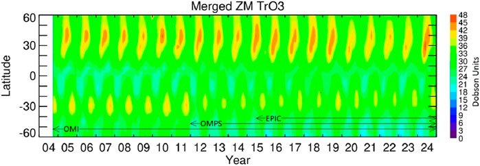
Figure 1. Merged monthly mean TCO derived from averaging the TCO products from EPIC (June 2015–December 2024), OMI (October 2004–December 2024), and OMPS (January 2012–December 2024). Merged TCO was derived using a simple equal-weighting averaging of the three sensors wherever mutual data were available. Both EPIC and OMPS TCO were pre-adjusted to OMI/MLS TCO by calculating the offsets at every 5^o × 5^o grid point based on pre-COVID years 2016–2019.

Deep convection associated with the inter-annual El Nino Southern Oscillation (ENSO), Indian Ocean dipole (IOD) events, the 1–2 months Madden–Julian oscillation (MJO), and year-round convection (with short timescales of days to weeks) forces large-scale changes in the tropospheric ozone of ∼5–15 DU within the tropics (Sekiya and Sudo, 2012; Ziemke et al., 2015, and references therein). The deep convection from these episodes uplifts boundary layer air with convective outflow in the mid-to-upper troposphere. The result is that tropospheric ozone concentrations throughout the vertical column are similar to BL concentrations over broad tropical areas. The convectively distributed ozone concentrations may, therefore, be small throughout much of the troposphere in the remote Pacific than in the regions of South America and Africa, which are much more polluted in the BL.

Weather systems in the extra-tropics result in year-round variability of ozone throughout the troposphere and lower stratosphere. The weather systems are initiated by baroclinic instabilities that are associated with the presence of horizontal temperature gradients on constant pressure surfaces (Holton, 2004). A characterization of weather system-related variability of tropospheric ozone, particularly satellite-derived TCO, has never been documented in literature. We include a short evaluation of weather-system variability in EPIC TCO to show related amplitudes and global spatial patterns.

Section 2 discusses the datasets used, Section 3 shows the results involving variabilities in TCO and evaluation of geostationary ozone measurements, and Section 4 summarizes our results.

2 Data

2.1 Satellite measurements of TCO

TCO from the DSCOVR EPIC instrument (Kramarova et al., 2021) is calculated by combining EPIC total column ozone with stratospheric ozone profiles from Global Modeling and Assimilation Office (GMAO) MERRA-2 (GMAO, 2015; Gelaro et al., 2017; Wargan et al., 2017). Synoptic hourly maps of TCO over the disk of the Earth are determined by subtracting coincident stratospheric column ozone (SCO) from total column ozone, where SCO is derived by vertically integrating MERRA-2-assimilated Aura MLS ozone profiles from the top of the atmosphere down to the tropopause. The tropopause pressure is taken from MERRA-2 analyses using standard potential vorticity–potential temperature (PV-θ) definition (i.e., 2.5 PV units or 380 K). The SCO synoptic fields from MERRA-2 at 3-h intervals are space–time co-located on a pixel-by-pixel basis via temporal interpolation with EPIC total ozone measurement footprints.

Sensitivity for detecting tropospheric ozone variability for EPIC is ∼100% above 5 km altitude but decreases to ∼40% for ozone columns below 5 km (Supplementary Figure S5). EPIC column weighing function (CWF) is reported for each EPIC total ozone measurement and indicates the measurements’ sensitivity to ozone changes in different atmospheric layers. TCO measured from EPIC/MERRA-2, therefore, represents mostly free tropospheric ozone. To account for the limited sensitivity to ozone variations in the boundary layer (BL) measured by EPIC, we applied a correction (ΔTCO), which is added to the derived hourly EPIC TCO columns (Kramarova et al., 2021, Supplemental): ∆TCO (λ, φ, t) = [1 – CWF₀(λ, φ, t)] ∗ [GEOS_CLIM(λ, φ, doy)-ML_CLIM(φ, doy)], where λ is the longitude, φ is the latitude, t is temporal index for EPIC measurements (Kramarova, et al., 2021, Supplemental), and doy is an index for day of year (1–365) for climatology. To retrieve EPIC total ozone, we use zonal mean climatology ML_CLIM (McPeters and Labow, 2012) that does not represent global variability in the BL ozone. Therefore, we created a gridded (at 1^o × 1^o) BL climatology GEOS_CLIM using GEOS-replay simulation (Molod et al., 2015) to compensate for the missing BL variability (for more details, see Kramarova et al., 2021).

The EPIC TCO synoptic maps gridded at 1^o × 1^o horizontal resolution are available to the general public from the NASA Langley Atmospheric Science Data Center (ASDC) (https://asdc.larc.nasa.gov/search?query=EPIC). The EPIC ozone observations were started in June 2015. EPIC did not make observations between late June 2019 and February 2020 due to malfunctioning of the satellite positioning. The observations were resumed in March 2020. In this study we also use daily gridded (1^o × 1^o) TCO maps calculated by averaging synoptic TCO maps for each day.

Our evaluation of EPIC TCO includes comparisons with OMI TCO (Ziemke et al., 2022) and OMPS TCO (McPeters et al., 2019; Elshorbany et al., 2021). We use SCO synoptic fields from MERRA-2 analyses for all three satellite products for consistency of TCO measurements. The TCO for both OMI and OMPS are calculated similarly to EPIC TCO by subtracting coincident MERRA-2 SCO from satellite Level-2 total ozone. Details of the OMI and OMPS TCO computations are discussed in Kramarova et al. (2021).

We have also used EPIC total ozone and TCO to evaluate similar measurements from the South Korean Geostationary Environmental Monitoring Spectrometer (GEMS) instrument launched on 19 February 2020. The GEMS geostationary instrument measures ozone and other trace gases at high spatiotemporal resolution in a region centered over East Asia (Baek et al., 2023). Horizontal resolution for GEMS is approximately 3.5 × 7 km². GEMS TCO for our study was derived similarly to EPIC TCO by subtracting space–time co-located MERRA-2 SCO from GEMS total ozone. An algorithm for directly deriving the GEMS profile ozone (not yet released to the public) is discussed in Bak et al. (2019).

2.2 Ozonesondes

As part of EPIC TCO validation, we have compared the EPIC TCO with ozonesonde measurements through 2024 from the World Ozone and Ultraviolet radiation Data Center (WOUDC), Southern Hemisphere Additional Ozonesondes (SHADOZ), and the Network for the Detection of Atmospheric Composition Change (NDACC). The sonde TCO is determined by integrating the daily sonde ozone mixing ratio from the ground level up to the tropopause, where the tropopause is defined the same as for EPIC TCO, that is, using co-located (at sonde location) MERRA-2 analyses and a standard PV-θ (2.5 PVU, 380 K) tropopause pressure definition. Most sonde ozone profile measurements are only once per day, with a total of approximately 1–4 profiles per month on average at each station. To colocate with the sondes, we use daily EPIC TCO maps and find the 1^o × 1^o grid box that encompasses the station location.

3 Results

3.1 Validation of EPIC/MERRA-2 TCO

EPIC/MERRA-2 TCO was studied previously by Kramarova et al. (2021) using both sonde and satellite TCO (e.g., OMI and OMPS) for the 2015–2020 time record. However, most of the sonde data for those comparisons were only available for a few years through at most mid-2019. Thus, for this study, we have updated the sonde evaluations of EPIC TCO through December 2024. Figure 2 shows time series of daily co-located EPIC TCO (black) and ozonesonde TCO (red) for several selected stations that have mostly continuous measurements over the EPIC 10-year record, with at least one sonde measurement per month on average over the 10-year record. Statistical offsets and standard deviations of EPIC/MERRA-2 TCO relative to ozonesondes for over 40 stations are listed in Supplementary Table S1. The panels in Figure 2 are arranged from the highest latitude to the lowest latitude from upper left to lower right. EPIC TCO (black asterisks) and sonde TCO (red asterisks) illustrate the dominant seasonal cycle present in TCO, which differs depending on the region. TCO in the NH can reach 50–60 DU at many stations, but TCO is low in the Southern Hemisphere (SH) Antarctic region at Davis (69^oS, 78^oE), with values as small as ∼5–10 DU in summer.

Figure 2

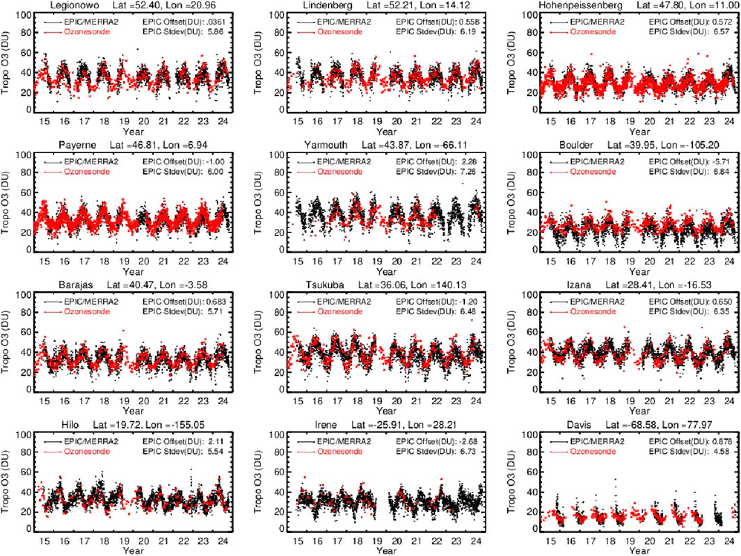
Figure 2. Time series of EPIC (black asterisks) and sondes (red asterisks) daily TCO for 2015–2024 at 12 selected ground-based locations (indicated). Mean offset and standard deviation in Dobson units for EPIC minus sonde TCO differences are quoted in each panel. This analysis uses daily ozonesondes from WOUDC, SHADOZ, and NDACC for the time period of 1 June 2015–31 December 2024.

Mean differences and standard deviations for the sonde comparisons are shown in Figure 3, where only the most continuous sondes through at least 2023 with at least one sonde measurement per month on average over the 10-year record were included in the analysis. Figure 3 reveals a systematic shape to the differences as a function of the latitude of several DU; however, given the ±1σ uncertainty bars of ∼5 DU, nearly all of the EPIC minus sonde differences, up to a few DU, are statistically not different from zero. We can conclude that EPIC daily-mean TCO agrees well with that of the daily sondes with a near-zero offset and standard deviations of ∼4–6 DU.

Figure 3

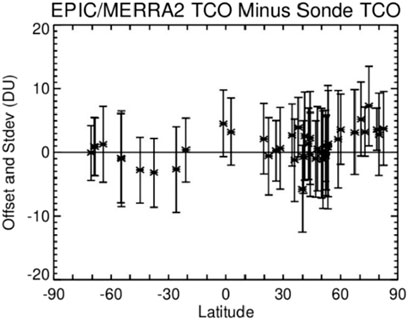
Figure 3. EPIC/MERRA-2 minus ozonesonde TCO differences (in Dobson units) calculated from daily co-located measurements. Sonde sites were chosen where the total number of sonde profile measurements over the 10-year record is at least 60 and extending through at least the year 2023. Vertical bars represent ±1σ standard deviation.

We have also compared EPIC TCO with OMI and OMPS TCO, as was done by Kramarova et al. (2021) for 2015–2020, but now with 10 years of EPIC data. Latitude-dependent mean differences between EPIC TCO and both OMI and OMPS TCO are shown in Figure 4 for selected months of the year. The curves in Figure 4 represent 10-year average differences in TCO for the months of January, April, July, and October. We note that the difference curves in Figure 4 are essentially identical to the difference curves for total column ozone since the same MERRA-2 SCO analyses fields are used to calculate all three TCO products. Each of the curves in Figure 4 for TCO closely compare to the curves in Figure 6 of Kramarova et al. (2021) for total ozone differences for the years 2015–2020. For the latitude range 60^oS–60^oN, in Figure 4, the EPIC, OMPS, and OMI TCO are on average within ±2–3 DU, with an exception for high SH latitudes, where the differences are ±3–6 DU. We conclude, as did Kramarova et al. (2021) from both satellite and sonde comparisons, that EPIC TCO appears to be overall well-calibrated for measuring TCO.

Figure 4

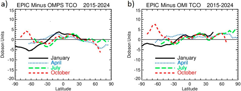
Figure 4. (a) EPIC/MERRA-2 TCO minus OMPS/MERRA-2 TCO (in Dobson units) 10-year averages for the months of January, April, July, and October (indicated). (b) Same as (a), but for OMI/MERRA-2 TCO. Because MERRA-2 SCO was used for all three satellite products, these TCO differences are essentially identical to differences in total column ozone.

3.2 TCO variabilities

TCO is always changing due to dynamics and photochemical sources that vary from daily to decadal timescales. In the tropics, most TCO variability originates from seasonal cycles coupled with ENSO and IOD and shorter daily to intra-seasonal changes that include the 1–2 month MJO (Tian et al., 2007; Ziemke and Chandra, 2003a; 2015; Fathurochman et al., 2017; Tweedy et al., 2020). Outside the tropics, TCO variability is mostly seasonal cycles with sources originating from seasonally varying stratosphere–troposphere exchange (STE), weather systems, and pollution events, including both anthropogenic and non-anthropogenic sources such as uncontrolled wildfires.

In the following sections, we derive characteristics of TCO variability from the 10 years of EPIC data beginning with basic seasonal cycles and ENSO signatures followed by using a multiple linear regression (MLR) model and calculated residuals to extract other remaining TCO variabilities.

3.2.1 Seasonal cycles

The largest and most persistent variability in tropospheric ozone originates from seasonal cycles due to seasonally varying stratospheric ozone influx and photochemical production in the troposphere. Seasonal cycles for EPIC TCO were determined from daily data by first computing the 2015–2024 average for each day of the year. The daily climatology was then averaged over 3-month seasons to produce the seasonal climatological maps shown in Figure 5. The seasonal cycle panels in Figure 5 for EPIC TCO can be compared with Supplementary Figure S1, S2 for OMI and OMPS TCO (discussed below).

Figure 5

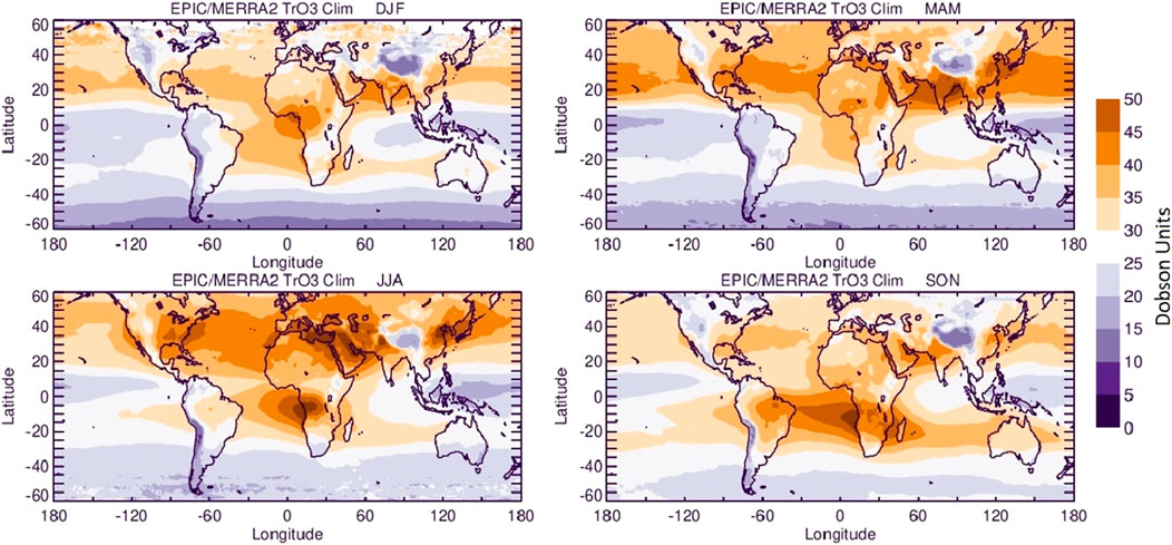
Figure 5. Seasonal TCO climatological maps (in Dobson units) calculated from 10 years of EPIC/MERRA-2 observations by averaging the climatological mean daily gridded (1^o × 1^o) EPIC/MERRA-2 TCO over 3-month periods: December–January–February (DJF), March–April–May (MAM), June–July–August (JJA), and September–October–November (SON).

NH TCO in Figure 5 is the greatest from spring (March–April–May, MAM) to summer (June–July–August, JJA), with largest ozone level occurring in the Mediterranean region during JJA. The Mediterranean in summer is known as an annually recurring accumulation “crossroads” region for pollution, including ozone precursors (Lelieveld et al., 2002). Terrain height is seen to reduce regional TCO by as much as ∼10–15 DU, such as over the Rocky Mountains in western N. America, the Asian Tibetan Plateau, and the S. American Andes. In the tropics and subtropics, the dominant signature in TCO is a zonal maximum in the Atlantic and minimum in the Pacific (i.e., zonal “wave one”). This wave-one pattern was first documented by Fishman et al. (1990). The wave-one in TCO is present year-round, with the largest amounts of ∼45 DU in the Atlantic in SON. Differences in TCO between the Atlantic and Pacific are also greatest during the SON (September–October–November) season, which is up to ∼25 DU. The structure and time dependence of the wave-one is due to the persistent tropical east–west Walker circulation, which controls the transport of ozone produced from STE, and ozone precursors produced by lightning and biomass burning into the tropical Atlantic Ocean region from Africa and S. America during the peak burning months (September–October) each year.

As further validation of EPIC TCO, we computed a zonal mean EPIC TCO climatology for each month and compared it with similar OMPS and OMI zonal mean TCO monthly climatologies averaged over the same time period of 2015–2024 (Figure 6). The Global Modeling Initiative (GMI) replay 12-month climatology is also included in Figure 6 for comparison. The GMI simulation climatology uses MERRA-2 meteorology and the same MERRA-2 tropopause with TCO derived by integrating model profile ozone from the ground up to the tropopause (Ziemke et al., 2015, and references therein).

Figure 6

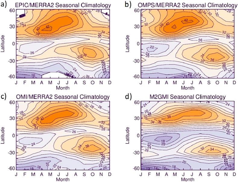
Figure 6. (a) Monthly zonal mean seasonal cycle in EPIC TCO (in DU) calculated from EPIC 1^o × 1^o gridded daily TCO data by averaging data over 2015–2024. (b) Same as (a), but for OMPS TCO. (c) Same as (a), but for OMI TCO. (d) Similar to (a), but for M2GMI simulated TCO (see text).

In the NH, in Figure 6, there is a distinct propagating phase shift of the seasonal peak from April to May in the subtropics to June to July at mid-latitudes for all three products and model. That is, in each case, the seasonal maximum in TCO exceeds 40 DU in April–May at approximately 25^oN, which extends into June–July at approximately 40^oN. This NH phase transition corresponds with a northward rate of approximately 5^o of latitude per month. The lowest TCO in the NH extra-tropics occurs in October–February at 50^oN–60^oN for all three products. In the SH, in Figure 6, the TCO seasonal cycle has the same phase with maxima during September–November at all latitudes for all three products and model; the largest SH TCO occurs at 15^oS–20^oS in September–November, with the amount being ∼36 DU. The lowest TCO in the SH is ∼15 DU and occurs at high latitudes around spring–summer months. The model simulation at high SH latitudes has a seasonal cycle close to that of EPIC and OMI and suggests that there may be some outlier measurements present for OMPS TCO at the high SH latitudes in winter when solar zenith angles for the satellite measurements are the largest. There are differences between the products and model in Figure 6 that involve mean bias differences and algorithm issues, but the patterns and amplitudes are all closely comparable between all four TCO panels. We summarize the seasonal variability in the tropics by noting the strong dependence on hemisphere, with TCO peaking in March–April in the NH and in September–November in the SH.

3.2.2 Inter-annual changes in tropical TCO due to ENSO and IOD

Tropical ENSO events and ensuing signatures on the ocean and atmosphere have been extensively studied and documented. Trenberth (1997) provided an extensive overview of ENSO with many key references. ENSO events in the tropics are known to generate substantial inter-annual anomalies in tropospheric ozone from satellites, sondes, and models (Chandra et al., 1998; 2002; Fujiwara et al., 1999; Thompson et al., 2001; Sudo and Takahashi, 2001; Nasser et al., 2009; Lee et al., 2010; Oman, et al., 2013; Ziemke and Chandra, 2003b; 2015; Le et al., 2024; Bruckner et al., 2024). Large ENSO-related increases in TCO reaching +20 DU over Indonesia in October 1997 have been recorded by Chandra et al. (2002) in ozonesondes, the Geostationary Earth Observation System Chemical transport model (GEOS-Chem), and Total Ozone Mapping Spectrometer (TOMS) satellite measurements. The GEOS-Chem model included in Chandra et al. (2002) indicated that most of the increases in TCO in the western Pacific during the 1997 El Nino occurred over Indonesia and originated from biomass burning, with the largest biomass burning contribution coming from above 5 km altitude.

We have studied inter-annual changes of EPIC TCO for 2015–2024 using de-seasonalized monthly-mean measurements. De-seasonalization of TCO was accomplished by subtracting mean seasonal cycles calculated from the 10-year record. Figure 7a compares time series of de-seasonalized TCO from EPIC (blue), OMI (red), and OMPS (black) for 2012–2024 in the tropical western Pacific at 100^oE and 5^oS, where the ENSO signal is large (discussed in Section 3.2.3). There were two strong El Nino events during this 10-year record, one in 2015 and one in 2023, with corresponding increases of 5–10 DU for all three products. La Nina events in late 2017 and 2020, seen as negative values in the Nino 3.4 index (Figure 7b), correspond with negative TCO anomalies of approximately −5 DU in the western Pacific.

Figure 7

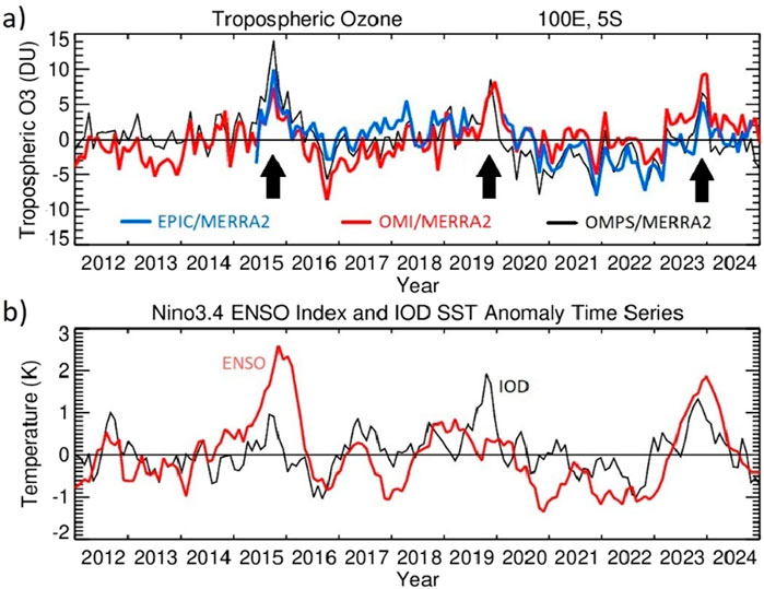
Figure 7. (a) De-seasonalized monthly TCO (in DU) in the tropical western Pacific (100^oE, 5^oS) for EPIC/MERRA-2 (blue curve), OMI/MERRA-2 (red curve), and OMPS/MERRA-2 (black curve). Here, the ENSO and IOD signals are both large (Section 3.2.3). The black arrows denote times when there were anomalously large increases (5–10 DU) in TCO corresponding to coupled positive phases of ENSO and IOD. (b) Monthly Nino 3.4 ENSO index (red curve) and IOD index (black curve) sea-surface temperature (SST) anomalies.

Another source of tropospheric ozone variability comes from the Indian Ocean Dipole (IOD) (Saji et al., 1999). A positive-phase IOD corresponds to enhanced convection just east of Africa, with suppressed convection toward the east over the Indian Ocean. The positive IOD in 2019 was among one of the most intense ever recorded and created drought conditions over northern Australia due to the induced lack of convection and rainfall (Lu and Ren, 2020). The increase in the IOD index (Figure 7b) corresponds to a positive TCO anomaly of approximately +5 DU in late 2019 due to suppressed convection over the tropical western Pacific region for both OMI and OMPS (note that there is a gap in EPIC data between late June 2019 and February 2020).

The black arrows in Figure 7 indicate the three largest (positive) TCO anomalies of +5 to +10 DU during this time period. These large positive anomalies in TCO coincide when the ENSO and IOD indices are both in a generally positive phase.

3.2.3 Other transient variabilities

We further study variabilities in EPIC TCO using a MLR model (e.g., Randel and Cobb, 1994, and references therein) to remove the dominant seasonal cycle and ENSO forcings to reveal other remaining variabilities. Prior to this MLR analysis, we re-gridded the EPIC daily TCO from 1^o × 1^o to 5^o × 5^o bin size to reduce computational time.

Table 1 shows the calculated correlations between the three TCO products and the individual ENSO and IOD indices from Figure 7. Correlations between IOD and TCO for all three products are small compared to correlations between ENSO and TCO. These small correlations coupled with redundancy between the IOD and ENSO indices (their cross-correlation is +0.47) suggests that we include only ENSO and not IOD as TCO proxies in our MLR analysis.

Table 1

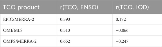
Table 1. Temporal correlation (r) between the TCO product time series in Figure 7 with both ENSO and IOD indices.

The MLR model that we use is $TCO\left(t\right)=A\left(t\right)+B·t+C·ENSO\left(t\right)+R\left(t\right)$, where t is the day index that runs between 1 January 2015 (t = 0) and 31 December 2024 (t = 3,653), A(t) is the seasonal-cycle fit, B is the linear trend coefficient, C is the ENSO coefficient, with ENSO(t) being the Nino 3.4 monthly time series extrapolated to daily, and R(t) represents the residual error term for the model. The seasonal cycle A(t) uses nine regression constants (a₀, a₁, …, a₈): A(t) = a₀ + a₁ cos(ωt) + a₂ sin(ωt) + a₃ cos(2ωt) + a₄ sin(2ωt) + a₅ cos(3ωt) + a₆ sin(3ωt) + a₇ cos(4ωt) + a₈ sin(4ωt), where the angular frequency ω = 2π/365. The other coefficients in the MLR model are simple constants. Any missing TCO data (such as during the earlier half of 2015 for EPIC) are not included in the regression. We include a linear trend term in the model, even though the record length for EPIC is too short to derive reliable trends.

Figure 8 shows a breakdown of the MLR model for each coefficient term including the original data TCO(t) time average (Figure 8a) and standard deviation of the MLR residual R(t) (Figure 8e). Figure 8a shows the 10-year average original data TCO, which can be compared with the 10-year seasonal climatology plotted in Figure 5. Figure 8b shows that the MLR model seasonal cycle compares closely with the original TCO in Figure 8a.

Figure 8

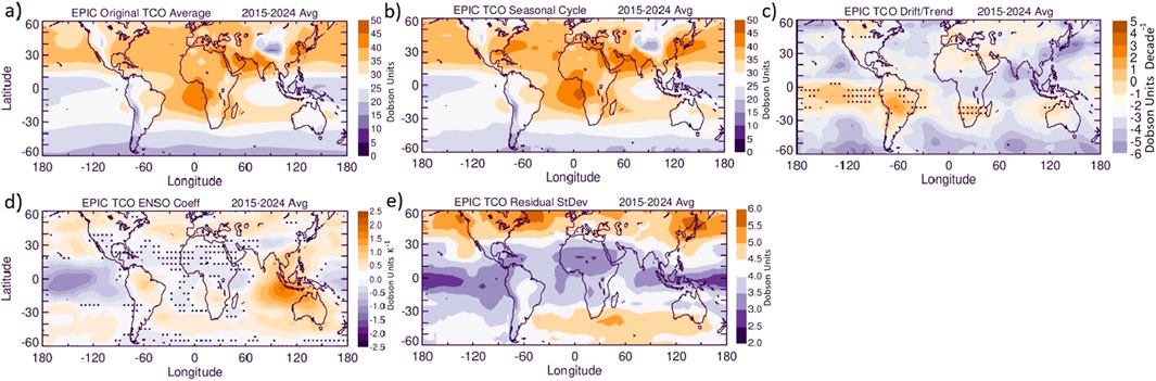
Figure 8. (a) Ten-year (2015–2024) average of EPIC original TCO measurements in Dobson units. (b) Similar 10-year average of the MLR seasonal-cycle fit. (c) Ten-year average of trend coefficient B in DU decade⁻¹. (d) Ten-year average MLR ENSO coefficient C in units DU K⁻¹. (e) Ten-year standard deviations of MLR residuals in Dobson units. Hatch marks denote regions where MLR coefficients are not different from zero at the 2σ level.

The linear trend term in Figure 8c suggests small increases in TCO in the tropics, with decreases in the extra-tropics of both hemispheres. The decrease in NH and SH TCO during 2015–2024 is consistent with anomalous drops in TCO of a few DU in both hemispheres starting in spring 2020 during the COVID-19 pandemic (Figure 1). Trends in global TCO have been reported in several articles published for the Tropospheric Ozone Assessment Report (TOAR-I and TOAR-II; https://igacproject.org/activities/TOAR/), where trends exhibit large variations in patterns and large differences between using different products. A main result from TOAR-II for the satellite, ground, and aircraft measurements is that TCO has been increasing over the East Asian region for several decades, with numbers varying from +1 to +4 DU decade⁻¹. TOAR-II focused on trends ending in 2019, while in this paper we consider 2015-2025. Most EPIC TCO trends in Figure 8c are not positive, but instead zero to negative and can be attributed to the short EPIC record coupled with effects from the 2-3 DU drops in NH TCO during COVID-19.

The ENSO coefficient in Figure 8d shows that ENSO variability in TCO is largely a tropical signal between the eastern and western Pacific. However, the ENSO signal in Figure 8d is not statistically zero outside the tropics. It is well known that the tropical ENSO affects meteorology in the extra-tropics (Vimont et al., 2003; Sun et al., 2021). The residual standard deviations in Figure 8e shows that the MLR model does well in simulating TCO in the tropics and subtropics with values of ∼2–4 DU (∼10% of background), but it becomes larger in higher latitudes, especially in high northern latitudes where numbers are closer to 5–6 DU (∼15%).

An additional way to evaluate the MLR results is to compare the spatial variability patterns for each model component. To do this, we compute the standard deviation of the reconstructed 10-year daily time series (t = 0–3,653 days) at each location for each term in the regression model, as shown in Figures 9b–e and compare to the standard deviation of the original TCO time series shown in Figure 9. Notably, the panels in Figure 9 have varying color bar scales. Figures 9a, b show the standard deviations for the original data and MLR seasonal cycle fit, respectively. Figures 9a, b show that the largest standard deviations for annual changes in TCO (up to ∼8 DU) occur over landmasses and along storm-track regions just east of the N. American and Asian continents. In comparison, the trend and ENSO terms have smaller standard deviations with trends showing wave structure outside the tropics, and ENSO again is associated mostly with the tropical Pacific region. ENSO standard deviations multiplied by a factor 4 are ∼5 DU, which results in approximate peak-to-peak average change from ENSO.

Figure 9

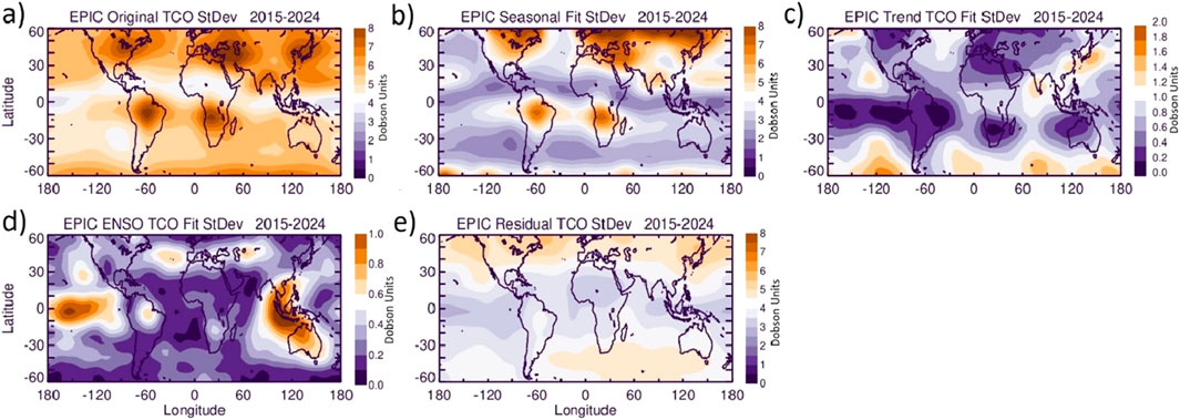
Figure 9. Calculated temporal standard deviations for (a) original EPIC TCO; (b) MLR seasonal cycle fit; (c) MLR linear trend fit; (d) MLR ENSO fit; (e) MLR residual. All standard deviations are in Dobson units. Figure 9e residuals have the same scaling as those of Figure 9a to better compare MLR error to the original data.

The standard deviations for MLR residuals in Figure 9e (same data as plotted in Figure 8e) are smaller than the original data variabilities (Figure 9a) and seasonal-cycle fit (Figure 9b) but are still up to 5 DU or greater in mid-high latitudes. The residuals show us that there are large variabilities present in daily TCO aside from just the seasonal cycles and ENSO forcing. Our further investigation of TCO variability uses the calculated residuals R(t) from the MLR model. The analysis includes both extra-tropical weather systems and the tropical 1–2 month MJO. We provide only a short overview of the mean amplitudes and geographical patterns associated with these forcings by applying bandpass filtering (Stanford and Vardeman, 1994) to the EPIC TCO 10-year record of daily residuals R(t) for 4–10 day and 30–60 day periods (Supplementary Figure S4). A detailed investigation of baroclinic weather systems and the MJO in tropospheric ozone is beyond the scope of our study.

Weather systems in both hemispheres are present year-round in atmospheric temperature, pressure, winds, and trace gases with characteristic oscillation periods of ∼4–10 days and large planetary scales involving east–west zonal wavenumbers of ∼4–10 (Andrews et al., 1987). We have estimated the average peak-to-peak changes in EPIC TCO associated with weather systems by first calculating standard deviation from bandpass filtered data and then scaling by a factor of 4 to approximate peak-to-peak change. Figure 10a shows a map of these changes for EPIC TCO associated with weather systems with 4–10-day periods. Figure 10a shows that TCO variations up to 10 DU occur throughout much of the SH and also over northern America and eastern Asia. The largest anomalies in TCO associated with weather systems have persistent patterns that are associated with natural topography, including the storm-track regions east of the continents of N. America and Asia. The percent changes in Figure 10c show that relative changes in the SH extra-tropical TCO due to weather systems may be up to 40% of the background amounts.

Figure 10

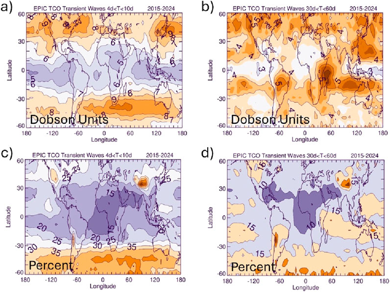
Figure 10. (a) EPIC transient wave variability (in Dobson units) calculated from daily 5^o × 5^o residual time series from the 1 January 2015–31 December 2024 MLR fit. The EPIC data were bandpass-filtered with half amplitude filter response at periods of 4 days and 10 days. Shown are the approximate peak-to-peak changes in TCO derived by calculating local standard deviation and multiplying this by 4. (b) Same as (a), but for the 30 d–60 d band. Bottom panels (c) and (d) show the percentage changes (relative to EPIC 10-year average TCO field) for (a) and (b), respectively.

Intra-seasonal variability in the tropics is dominated by the 1–2 month MJO, known historically as the 40–50 day MJO (Madden and Julian, 1972; 1971). Madden and Julian (1994) provide a detailed overview of MJO effects on the ocean and atmosphere. The MJO is associated with anomalous deep convection in the tropics driven by ocean–atmosphere feedback coupling with convection cells starting in the Indian Ocean and propagating eastward across the dateline into the eastern Pacific with periods averaging approximately 45 days. The largest MJO signal in meteorological parameters (winds, temperatures, and pressures) occurs during northern winter months; however, this oscillation is present year-round.

Figure 10b shows bandpass-filtered EPIC TCO for the period of 30–60 days to estimate peak-to-peak amplitudes in the tropics and subtropics associated with the MJO. The 1–2-month signals in TCO in Figure 10b are generally tropical compared to patterns associated with weather systems (Figure 10a), and they also have a smaller magnitude of variations of ∼5 DU. At high NH latitudes, in Figure 10b, the signal is up to ∼4 DU. Studies have shown that the MJO impacts dynamical events including blocking in NH high latitudes (Henderson and Maloney, 2018, and references therein), so we cannot rule out that the observed TCO anomalies in high NH latitudes (Figure 10b) are related to MJO. Figure 10d shows associated percentage changes relative to mean background ozone. Large percentage changes that occur in high southern latitudes in Figure 10d are due to small background TCO amounts year-round.

3.3 Evaluation of GEMS and EPIC tropospheric ozone synoptic hourly maps

The 1–2 hourly sampling for EPIC yields, on average, approximately 3–4 and up to 8–10 daytime TCO and total ozone measurements per day at a given location on the Earth’s surface (within local noon ±6 h). The high sampling rate makes EPIC useful for evaluating ozone measurements from geostationary satellite instruments including the current GEMS (Korean instrument centered over east Asia; Kim et al., 2024, and references therein) and TEMPO (NASA/Smithsonian Astrophysical Observatory instrument centered over North America; Zhao et al., 2025, and references therein). We have compared EPIC with both TEMPO and GEMS hourly measurements of TCO. The current TEMPO version 3 total ozone measurement has some remaining issues, including a strong latitudinally varying offset of 10–15 DU; for this reason, we only analyze EPIC with GEMS total ozone and TCO. As with EPIC TCO, the GEMS TCO was derived by subtracting coincident MERRA-2 SCO from GEMS level-2 total column ozone. Both products use the same tropopause based on MERRA-2 meteorology using 2.5 PVU and 380 K surfaces. The GEMS total column ozone was first gridded at 0.1 × 0.1 resolution, and then, MERRA-2 SCO was interpolated and matched in both space and time to generate GEMS TCO.

Figure 11a shows GEMS TCO centered over East Asia on 22 May 2021 at 11:00 local time (top panel) and 15:00 local time (bottom panel). The GEMS TCO exhibits strong horizontal gradients with fine structures and patterns. Figure 11b shows corresponding EPIC TCO (standard product) for the same region and times as GEMS. EPIC has similar qualitative patterns as GEMS TCO in Figure 11a, but many small features seen in GEMS TCO are not present in EPIC TCO due to the coarse spatial resolution of EPIC.

Figure 11

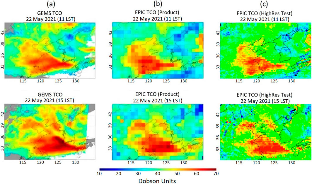
Figure 11. (a) TCO from GEMS (in DU) at 11:00 local standard time (LST) (top panel) and 15:00 LST (lower panel) on 22 May 2021. (b) Same as (a), but for the EPIC TCO standard 1^o × 1^o product. (c) Same as (a), but for the EPIC TCO high-resolution 0.25^o × 0.25^o test product.

We have tested EPIC TCO at a higher resolution of 0.25^o × 0.25^o rather than the 1^o × 1^o of the standard product to better compare it with GEMS TCO. Figure 11c shows that increasing the resolution for EPIC TCO does better than the EPIC standard product for resolving small anomalies. GEMS TCO also detects some small features (especially at 15 LST), which may be due to EPIC having less sensitivity to ozone in the low troposphere. Our analyses show good consistency between GEMS and EPIC TCO and that the current EPIC TCO product may be improved by increasing the resolution from 1^o × 1^o to 0.25^o × 0.25^o. We note that the 1^o × 1^o product has estimated local precision errors of approximately 2.5 DU in daily maps (Kramarova et al., 2021); these errors are larger for the 0.25^o × 0.25^o product by approximately 4 due to having 16 times as many gridpoints.

4 Summary

EPIC measures total column ozone over the sunlit disk of the Earth every 1–2 h as synoptic data images, providing, on average, approximately 3–4 measurements (up to 8–10 in NH summer) of total column ozone every day at a given fixed surface location. This hourly sampling rate coupled with near-global coverage each day and long decadal record is unique among existing satellite instruments. EPIC level-2 hourly total ozone is combined with MERRA-2 SCO to generate TCO for the time period of June 2015–December 2025. The TCO level-2 data are gridded to 1^o × 1^o resolution maps with the same 1–2 hourly sampling for analysis. Validation of EPIC TCO was accomplished using TCO from ozonesondes and other satellite measurements (e.g., OMI and OMPS).

Our study provides a characterization of dominant variabilities present in TCO using the 10 years of EPIC observations. We included an MLR model to delineate patterns and amplitudes for these different forcings. The TCO variabilities investigated include seasonal cycles, trends, inter-annual ENSO and IOD, extra-tropical weather systems, and the tropical 1–2 month MJO. We studied these variabilities to both test the quality of the EPIC TCO data and provide new scientific results.

The largest variability in TCO originates from seasonal cycles, where typical annual changes are 20–30 DU and tend to be located over land masses and along oceanic storm-track regions. ENSO largely affects TCO in the tropical Pacific region, with typical anomalies of ∼5–10 DU during either El Nino or La Nina events. Our analysis shows that ENSO variability detected from EPIC TCO engulfs the broad tropical western and eastern Pacific regions, which is in agreement with previous studies. With weather systems, we found typical peak-to-peak TCO variations of ∼10 DU on average in mid-latitudes of both hemispheres. The changes in TCO caused by weather systems have a greater relative impact in the SH, with peak-to-peak variations up to 40% of the mean background ozone. In comparison, the tropical 1–2-month MJO shows that the most variability occurs in the tropics, with peak-to-peak amplitudes of approximately 5–10 DU on average.

Starting in 2020, EPIC TCO shows a drop of 2–3 DU during spring–summer months throughout the NH, which appears to have continued seasonally through 2023, with TCO in spring–summer 2024 being back to pre-COVID levels. Although only a 2–3 DU drop, this anomaly affects trend calculations in the NH for TCO data that include these years. Our MLR analysis of EPIC TCO shows a corresponding slight decrease in NH extra-tropical TCO for 2015–2024; however, the 10-year record may be too short for meaningful trends.

The EPIC total ozone and TCO with a 1–2 h sampling rate is also useful for evaluating similar data from geostationary satellites. We have compared EPIC hourly TCO with geostationary GEMS TCO (centered over East Asia). The GEMS TCO shows sub-city resolution details and evidence of small propagating ozone plumes. The EPIC TCO hourly product is gridded at 1^o × 1^o and compares well with GEMS TCO for broad-scale, but not urban-scale features. We tested changing the EPIC TCO resolution to 0.25^o × 0.25^o, which is near the resolution limit for EPIC ozone measurements (∼18 km × 18 km resolution for nadir satellite view). The higher-resolution EPIC TCO can capture smaller scale features seen in GEMS TCO that the coarser gridded EPIC TCO cannot. Going forward, we will continue to develop and optimize the high resolution measurements from EPIC.

Data availability statement

The EPIC tropospheric ozone hourly data for June 2015-present are available from the NASA Langley Atmospheric Science Data Center (ASDC) https://asdc.larc.nasa.gov/. The EPIC, OMI/MLS, and OMPS tropospheric ozone monthly-mean products used in this study are currently available from the NASA Goddard satellite tropospheric ozone webpage (https://acd-ext.gsfc.nasa.gov/Data_services/cloud_slice/. MERRA-2 meteorological fields and profile ozone from assimilation are available from NASA Goddard Modeling and Assimilation Office (GMAO) at website https://gmao.gsfc.nasa.gov/.

Author contributions

JZ: writing – original draft and writing – review and editing. NK: writing – review and editing and writing – original draft. SF: writing – review and editing and writing – original draft. K-LH: writing – original draft and writing – review and editing. KB: writing – review and editing and writing – original draft. JH: writing – original draft and writing – review and editing.

Funding

The author(s) declare that financial support was received for the research and/or publication of this article. This research has been supported by the NASA programmatic fund “Long-term ozone trends” (project no. WBS 479717). JZ and NK were also supported by the NASA ROSES proposal “Continuing total and tropospheric ozone column products from DSCOVR EPIC to study regional scale ozone transport (NNH21ZDA001N-DSCOVR:A.25 DSCOVR Science Team. SF was supported under NASA contract NNG17HP01C.

Acknowledgments

The authors thank the NASA Jet Propulsion Laboratory MLS team for the MLS v4.2 ozone dataset and the EPIC, OMPS, and OMI ozone processing teams. MERRA-2 is an official product of the Global Modeling and Assimilation Office at NASA GSFC. The authors also thank the NASA Center for Climate Simulation (NCCS) for providing high-performance computing resources.

Conflict of interest

Authors SF and K-LH were employed by Science Systems and Applications Inc. (SSAI). Authors KB and JH were employed by University of Maryland Baltimore Co.

The remaining authors declare that the research was conducted in the absence of any commercial or financial relationships that could be construed as a potential conflict of interest.

The handling editor AL declared a shared affiliation with the authors at the time of review.

Generative AI statement

The author(s) declare that no Generative AI was used in the creation of this manuscript.

Publisher’s note

All claims expressed in this article are solely those of the authors and do not necessarily represent those of their affiliated organizations, or those of the publisher, the editors and the reviewers. Any product that may be evaluated in this article, or claim that may be made by its manufacturer, is not guaranteed or endorsed by the publisher.

Supplementary material

The Supplementary Material for this article can be found online at: https://www.frontiersin.org/articles/10.3389/frsen.2025.1634922/full#supplementary-material

References

Andrews, D. G., Holton, J. R., and Leovy, C. B. (1987). Middle atmosphere dynamics. San Diego, Calif: Academic, 489.

Google Scholar

Baek, K., Kim, J. H., Bak, J., Haffner, D. P., Kang, M., and Hong, H. (2023). Evaluation of total ozone measurements from geostationary environmental monitoring spectrometer (GEMS). Atmos. Meas. Tech. 16, 5461–5478. doi:10.5194/amt-16-5461-2023

CrossRef Full Text | Google Scholar

Bak, J., Baek, K.-H., Kim, J.-H., Liu, X., Kim, J., and Chance, K. (2019). Cross-evaluation of GEMS tropospheric ozone retrieval performance using OMI data and the use of an ozonesonde dataset over East Asia for validation. Atmos. Meas. Tech. 12, 5201–5215. doi:10.5194/amt-12-5201-2019

CrossRef Full Text | Google Scholar

Bauwens, M., Compernolle, S. T., Müller, J.-F., van Gent, J., Eskes, H., Levelt, P. F., et al. (2020). Impact of coronavirus outbreak on NO₂ pollution assessed using TROPOMI and OMI observations. Geophys. Res. Lett. 47, e2020GL087978. doi:10.1029/2020GL087978

PubMed Abstract | CrossRef Full Text | Google Scholar

Bouarar, I., Gaubert, B., Brasseur, G. P., Steinbrecht, W., Doumbia, T., Tilmes, S., et al. (2021). Ozone anomalies in the free troposphere during the COVID-19 pandemic. Geophys. Res. Lett. 48 (16), e2021GL094204. doi:10.1029/2021GL094204

CrossRef Full Text | Google Scholar

Bray, C. D., Nahas, A., Battye, W. H., and Aneja, V. P. (2021). Impact of lockdown during the COVID-19 outbreak on multi-scale air quality. Atmos. Environ. 254, 118386. doi:10.1016/j.atmosenv.2021.118386

PubMed Abstract | CrossRef Full Text | Google Scholar

Bruckner, M., Pierce, R. B., and Lenzen, A. (2024). Examining ENSO-related variability in tropical tropospheric ozone in the RAQMS-Aura chemical reanalysis. Atmos. Chem. Phys. 24, 10921–10945. doi:10.5194/acp-24-10921-2024

CrossRef Full Text | Google Scholar

Campbell, P. C., Tong, D., Tang, Y., Baker, B., Lee, P., Saylor, R., et al. (2021). Impacts of the COVID-19 economic slowdown on ozone pollution in the U.S. U.S. Atmos. Environ. 264, 118713. doi:10.1016/j.atmosenv.2021.118713

PubMed Abstract | CrossRef Full Text | Google Scholar

Chandra, S., Ziemke, J. R., Bhartia, P. K., and Martin, R. V. (2002). Tropical tropospheric ozone: implications for dynamics and biomass burning. J. Geophys. Res. 107 (D14), 4188. doi:10.1029/2001jd000447

CrossRef Full Text | Google Scholar

Chandra, S., Ziemke, J. R., Min, W., and Read, W. G. (1998). Effects of 1997–1998 El Niño on tropospheric ozone and water vapor. Geophys. Res. Lett. 25, 3867–3870. doi:10.1029/98GL02695

CrossRef Full Text | Google Scholar

Elshorbany, Y. Y., Kapper, H. C., Ziemke, J. R., and Parr, S. A. (2021). The status of air quality in the United States during the COVID-19 pandemic: a remote sensing perspective. Rem. Sens. 13 (3), 369. doi:10.3390/rs13030369

CrossRef Full Text | Google Scholar

Fathurochman, I., Lubis, S. W., and Setiawan, S. (2017). Impact of Madden-Julian Oscillation (MJO) on global distribution of total water vapor and column ozone. IOP Conf. Ser. Earth Environ. Sci. 54, 012034. doi:10.1088/1755-1315/54/1/012034

CrossRef Full Text | Google Scholar

Fishman, J., Watson, C. E., Larsen, J. C., and Logan, J. A. (1990). Distribution of tropospheric ozone determined from satellite data. J. Geophys. Res. 95, 3599–3617. doi:10.1029/JD095iD04p03599

CrossRef Full Text | Google Scholar

Fujiwara, M., Kita, K., Kawakami, S., Ogawa, T., Komala, N., Saraspriya, S., et al. (1999). Tropospheric ozone enhancements during the Indonesian forest fire events in 1994 and in 1997 as revealed by ground-based observations. Geophys. Res. Lett. 26, 2417–2420. doi:10.1029/1999GL900117

CrossRef Full Text | Google Scholar

Gelaro, R., McCarty, W., Suárez, M. J., Todling, R., Molod, A., Takacs, L., et al. (2017). The Modern-Era Retrospective analysis for research and Applications, version 2 (MERRA-2). J. Clim. 30, 5419–5454. doi:10.1175/JCLI-D-16-0758.1

PubMed Abstract | CrossRef Full Text | Google Scholar

Global Modeling and Assimilation Office (GMAO) (2015). MERRA-2 inst3_3d_asm_Nv: 3d,3-hourly, instantaneous, model-level, assimilation, assimilated meteorological fields V5.12.4. Greenbelt, MD, USA: Goddard Earth Sciences Data and Information Services Center GES DISC. doi:10.5067/WWQSXQ8IVFW8

CrossRef Full Text | Google Scholar

Henderson, S. A., and Maloney, E. D. (2018). The impact of the madden–julian oscillation on high-latitude winter blocking during El niño–southern oscillation events. J. Clim. 31, 5293–5318. doi:10.1175/JCLI-D-17-0721.1

CrossRef Full Text | Google Scholar

Herman, J., Huang, L., McPeters, R., Ziemke, J., Cede, A., and Blank, K. (2018). Synoptic ozone, cloud reflectivity, and erythemal irradiance from sunrise to sunset for the whole earth as viewed by the DSCOVR spacecraft from the earth–sun Lagrange 1 orbit. Atmos. Meas. Tech. 11, 177–194. doi:10.5194/amt-11-177-2018

CrossRef Full Text | Google Scholar

Holton, J. R. (2004). An introduction to dynamic meteorology. 4th Ed. Burlington, MA, USA: Elsevier Academic Press, 529.

Google Scholar

Jensen, A., Liu, Z., Tan, W., Dix, B., Chen, T., Koss, A., et al. (2021). Measurements of volatile organic compounds during the COVID-19 lock-down in Changzhou, China. Geophys. Res. Lett. 48 (20), e2021GL095560. doi:10.1029/2021GL095560

PubMed Abstract | CrossRef Full Text | Google Scholar

Keller, C. A., Evans, M. J., Knowland, K. E., Hasenkopf, C. A., Modekurty, S., Lucchesi, R. A., et al. (2021). Global impact of COVID-19 restrictions on the surface concentrations of nitrogen dioxide and ozone. Atmos. Chem. Phys. 21 (5), 3555–3592. doi:10.5194/acp-21-3555-2021

CrossRef Full Text | Google Scholar

Kim, J., Oh, S., Bak, J., Koo, J.-H., Park, S. S., and Lee, W.-J. (2024). GEMS ozone product evaluation using ozonesonde measurements during the ACCLIP campaign. EGU General Assem. 2024 (14–19), Vienna, Austria, EGU24–7138. doi:10.5194/egusphere-egu24-7138

CrossRef Full Text | Google Scholar

Kramarova, N. A., Ziemke, J. R., Huang, L.-K., Herman, J. R., Wargan, K., Seftor, C. J., et al. (2021). Evaluation of version 3 total and tropospheric ozone columns from earth polychromatic imaging Camera on deep space climate observatory for studying regional scale ozone variations. Front. Rem. Sens. 2, 734071. doi:10.3389/frsen.2021.734071

CrossRef Full Text | Google Scholar

Le, T., Kim, S.-H., Heo, J.-Y., and Bae, D.-H. (2024). The influences of El Niño–Southern Oscillation on tropospheric ozone in CMIP6 models. Atmos. Chem. Phys. 24, 6555–6566. doi:10.5194/acp-24-6555-2024

CrossRef Full Text | Google Scholar

Lee, S., Shelow, D. M., Thompson, A. M., and Miller, S. K. (2010). QBO and ENSO variability in temperature and ozone from SHADOZ, 1998-2005. J. Geophys. Res. 115, D18105. doi:10.1029/2009JD013320

CrossRef Full Text | Google Scholar

Lelieveld, J., Berresheim, H., Borrmann, S., Crutzen, P. J., Dentener, F. J., Fischer, H., et al. (2002). Global air pollution crossroads over the Mediterranean. Science 298, 794–799. doi:10.1126/science.1075457

PubMed Abstract | CrossRef Full Text | Google Scholar

Liu, F., Page, A., Strode, S. A., Yoshida, Y., Choi, S., Zheng, B., et al. (2020). Abrupt decline in tropospheric nitrogen dioxide over China after the outbreak of COVID-19. Sci. Adv. 6, eabc2992. doi:10.1126/sciadv.abc2992

PubMed Abstract | CrossRef Full Text | Google Scholar

Lu, B., and Ren, H.-L. (2020). What caused the extreme Indian Ocean Dipole event in 2019? Geophys. Res. Lett. 47. doi:10.1029/2020GL087768

CrossRef Full Text | Google Scholar

Madden, R. A., and Julian, P. R. (1972). Description of global-scale circulation cells in the tropics with a 40–50 day period. J. Atmo. Sci. 29, 1109–1123. doi:10.1175/1520-0469(1972)029<1109:DOGSCC>2.0.CO;2

CrossRef Full Text | Google Scholar

Madden, R. A., and Julian, P. R. (1972). Description of global-scale circulation cells in the tropics with a 40–50 Day period. CO, 1109–1123. doi:10.1175/1520-0469(1972)029<1109:DOGSCC>2.0

CrossRef Full Text | Google Scholar

Madden, R. A., and Julian, P. R. (1994). Observations of the 40–50 day tropical oscillation-a review. Mon. Weather Rev. 122, 814–837. doi:10.1175/1520-0493(1994)122<0814:ootdto>2.0.co;2

CrossRef Full Text | Google Scholar

Marshak, A., Herman, J. R., Adams, S., Blank, K., Carn, S., Cede, A., et al. (2018). Earth observations from DSCOVR EPIC instrument. Bull. Amer. Meteor. Soc. 99, 1829–1850. doi:10.1175/BAMS-D-17-0223.1

CrossRef Full Text | Google Scholar

McPeters, R. D., and Labow, G. J. (2012). Climatology 2012: An MLS and sonde derived ozone climatology for satellite retrieval algorithms. J. Geophys. Res. 117. doi:10.1029/2011JD017006

CrossRef Full Text | Google Scholar

McPeters, R. D., Frith, S. M., Kramarova, N. A., Ziemke, J. R., and Labow, G. J. (2019). Trend quality ozone from NPP OMPS: the version 2 processing. Atmos. Meas. Tech. 12, 977–985. doi:10.5194/amt-12-977-2019

CrossRef Full Text | Google Scholar

Miyazaki, K., Bowman, K., Sekiya, T., Takigawa, M., Neu, J. L., Sudo, K., et al. (2021). Global tropospheric ozone responses to reduced NO_x emissions linked to the COVID-19 worldwide lockdowns. Sci. Adv. 7 (24), eabf7460. doi:10.1126/sciadv.abf7460

PubMed Abstract | CrossRef Full Text | Google Scholar

Molod, A., Takacs, L., Suarez, M., and Bacmeister, J. (2015). Development of the GEOS-5 atmospheric general circulation model: evolution from MERRA to MERRA2. Geosci. Model Dev. 8, 1339–1356. doi:10.5194/gmd-8-1339-2015

CrossRef Full Text | Google Scholar

Nasser, R., Logan, J. A., Megratskaia, I. A., Murray, L. T., Zhang, L., and Jones, D. B. A. (2009). Analysis of tropical tropospheric ozone, carbon monoxide, and water vapor during the 2006 El Niño using TES observations and the GEOS-Chem model. J. Geophys. Res. 114, D17304. doi:10.1029/2009JD011760

CrossRef Full Text | Google Scholar

Oman, L. D., Douglass, A. R., Ziemke, J. R., Rodriguez, J. M., Waugh, D. W., and Nielsen, J. E. (2013). The ozone response to ENSO in Aura satellite measurements and a chemistry climate simulation. J. Geophys. Res. 118, 965–976. doi:10.1029/2012JD018546

CrossRef Full Text | Google Scholar

Pakkattil, A., Muhsin, M., and Ravi Varma, M. K. (2021). COVID-19 lockdown: effects on selected volatile organic compound (VOC) emissions over the major Indian metro cities. Urban Clim. 37, 100838. doi:10.1016/j.uclim.2021.100838

PubMed Abstract | CrossRef Full Text | Google Scholar

Randel, W. J., and Cobb, J. B. (1994). Coherent variations of monthly mean total ozone and lower stratospheric temperature. J. Geophys. Res. 99, 5433–5447. doi:10.1029/93JD03454

CrossRef Full Text | Google Scholar

Saji, N. H., Goswami, B. N., Vinayachandran, P. N., and Yamagata, T. (1999). A dipole mode in the tropical Indian Ocean. Nature 401, 360–363. doi:10.1038/43854

PubMed Abstract | CrossRef Full Text | Google Scholar

Sekiya, T., and Sudo, K. (2012). Role of meteorological variability in global tropospheric ozone during 1970–2008. J. Geophys. Res. 117. doi:10.1029/2012JD018054

CrossRef Full Text | Google Scholar

Sicard, P., De Marco, A., Agathokleous, E., Feng, Z., Xu, X., Paoletti, E., et al. (2020). Amplified ozone pollution in cities during the COVID-19 lockdown. Sci. Total Environ. 735, 139542. doi:10.1016/j.scitotenv.2020.139542

PubMed Abstract | CrossRef Full Text | Google Scholar

Stanford, J. L., and Vardeman, S. B. (1994). in Statistical methods for physical science. Editors J. L. Stanford, and S. B. Vardeman (New York: Academic Press, Inc.), 528.

Google Scholar

Stavrakou, T., Müller, J.-F., Bauwens, M., Doumbia, T., Elguindi, N., Darras, S., et al. (2021). Atmospheric impacts of COVID-19 on NO_x and VOC levels over China based on TROPOMI and IASI satellite data and modeling. Atmosphere 12 (8), 946. doi:10.3390/atmos12080946

CrossRef Full Text | Google Scholar

Steinbrecht, W., Kubistin, D., Plass-Dülmer, C., Davies, J., Tarasick, D. W., von der Gathen, P., et al. (2021). COVID-19 crisis reduces free tropospheric ozone across the Northern Hemisphere. Geophys. Res. Lett. 48 (5), e2020GL091987. doi:10.1029/2020GL091987

PubMed Abstract | CrossRef Full Text | Google Scholar

Sudo, K., and Takahashi, M. (2001). Simulation of tropospheric ozone changes during 1997–1998 El Niño: meteorological impact on tropospheric photochemistry. Geophys. Res. Lett. 28, 4091–4094. doi:10.1029/2001gl013335

CrossRef Full Text | Google Scholar

Sun, L., Yang, X.-Q., Tao, L., Fang, J., and Sun, X. (2021). Changing impact of ENSO events on the following summer rainfall in eastern China since the 1950s, J. Clim. 34, 8105–8123. doi:10.1175/JCLI-D-21-0018.1

CrossRef Full Text | Google Scholar

Sun, W., Jiang, W., and Li, R. (2024). Global health benefits of shipping emission reduction in early 2020. Atmos. Env. 333, 120648. doi:10.1016/j.atmosenv.2024.120648

CrossRef Full Text | Google Scholar

Thompson, A. M., Witte, J. C., Hudson, R. D., Guo, H., Herman, J. R., and Fujiwara, M. (2001). Tropical tropospheric ozone and biomass burning. Science 291 (5511), 2128–2132. doi:10.1126/science.291.5511.2128

PubMed Abstract | CrossRef Full Text | Google Scholar

Tian, B., Yung, Y. L., Waliser, D. E., Tyranowski, T., Kuai, L., Fetzer, E. J., et al. (2007). Intraseasonal variations of the tropical total ozone and their connection to the Madden-Julian Oscillation. Geophys. Res. Lett. 34. doi:10.1029/2007GL029451

CrossRef Full Text | Google Scholar

Trenberth, K. E. (1997). The definition of El niño. B. Am. Meteorol. Soc. 78 (2), 2771–2777. doi:10.1175/1520-0477(1997)078

CrossRef Full Text | Google Scholar

Tweedy, O. V., Oman, L. D., and Waugh, D. W. (2020). Seasonality of the MJO impact on upper troposphere–lower stratosphere temperature, circulation, and composition. J. Atmos. Sci. 77, 1455–1473. doi:10.1175/JAS-D-19-0183.1

CrossRef Full Text | Google Scholar

Vimont, D. J., Wallace, J. M., and Battisti, D. S. (2003). The seasonal footprinting mechanism in the Pacific: implications for ENSO. J. Clim. 16, 2668–2675. doi:10.1175/1520-0442(2003)016

CrossRef Full Text | Google Scholar

Wargan, K., Labow, G., Frith, S., Pawson, S., Livesey, N., and Partyka, G. (2017). Evaluation of the ozone fields in NASA’s MERRA-2 reanalysis. J. Clim. 30 (8), 2961–2988. doi:10.1175/JCLI-D-16-0699.1

PubMed Abstract | CrossRef Full Text | Google Scholar

Zhao, X., Griffin, D., Fioletov, V., McLinden, C., Liu, X., Park, J., et al. (2025). Geostationary satellites total ozone observations: first results on ground-based networks validation efforts for TEMPO and GEMS. Geophys. Res. Lett. 52, e2025GL114768. doi:10.1029/2025GL114768

PubMed Abstract | CrossRef Full Text | Google Scholar

Ziemke, J. R., and Chandra, S. (2003a). A Madden-Julian Oscillation in tropospheric ozone. Geophys. Res. Lett. 30 (23), 2182. doi:10.1029/2003GL018523

CrossRef Full Text | Google Scholar

Ziemke, J. R., and Chandra, S. (2003b). La Nina and El Nino induced variabilities of ozone in the tropical lower atmosphere during 1970-2001. Geophys. Res. Lett. 30 (3), 1142. doi:10.1029/2002GL016387

CrossRef Full Text | Google Scholar

Ziemke, J. R., Douglass, A. R., Oman, L. D., Strahan, S. E., and Duncan, B. N. (2015). Tropospheric ozone variability in the tropics from ENSO to MJO and shorter timescales. Atmos. Chem. Phys. 15, 8037–8049. doi:10.5194/acp-15-8037-2015

CrossRef Full Text | Google Scholar

Ziemke, J. R., Kramarova, N. A., Frith, S. M., Huang, L.-K., Haffner, D. P., Wargan, K., et al. (2022). NASA satellite measurements show global-scale reductions in free tropospheric ozone in 2020 and again in 2021 during COVID-19. Geophys. Res. Lett. 49, e2022GL098712. doi:10.1029/2022GL098712

PubMed Abstract | CrossRef Full Text | Google Scholar