The single beacon: progresses in understanding Earth as an exoplanet using DSCOVR/EPIC observations

Jian, Xun; Gu, Lixiang; Fan, Siteng; Bartlett, Stuart J.; Yang, Jiani; Jiang, Jonathan H.; Luo, Yangcheng; Yung, Yuk L.

doi:10.3389/frsen.2025.1635015

REVIEW article

Front. Remote Sens., 08 August 2025

Sec. Multi- and Hyper-Spectral Imaging

Volume 6 - 2025 | https://doi.org/10.3389/frsen.2025.1635015

This article is part of the Research TopicEarth Observations from the Deep Space: 10 Years of the DSCOVR MissionView all 4 articles

The single beacon: progresses in understanding Earth as an exoplanet using DSCOVR/EPIC observations

Xun Jian^1,2

Lixiang Gu¹

Siteng Fan¹*

Stuart J. Bartlett²

Jiani Yang²

Jonathan H. Jiang³

Yangcheng Luo⁴

Yuk L. Yung^2,3

¹Department of Earth and Space Sciences, Southern University of Science and Technology, Shenzhen, Guangdong, China
²Division of Geological and Planetary Sciences, California Institute of Technology, Pasadena, CA, United States
³Jet Propulsion Laboratory, California Institute of Technology, Pasadena, CA, United States
⁴Laboratoire de Météorologie Dynamique (LMD)/Institut Pierre-Simon Laplace (IPSL), École Normale Supérieure (ENS), Université Paris Sciences et Lettres (PSL), Centre National de la Recherche Scientifique (CNRS), Institut Polytechnique de Paris, Sorbonne Université, Paris, France

Almost 6000 exoplanets have thus far been confirmed, revolutionizing our understanding of planetary habitability. Yet, despite the identification of Earth-like exoplanets, definitive evidence of extraterrestrial life remains elusive. Studying Earth, the only confirmed habitable and inhabited planet, as a proxy exoplanet provides critical insights for interpreting forthcoming exoplanet direct-imaging data. Observations from the Deep Space Climate Observatory/Earth Polychromatic Imaging Camera (DSCOVR/EPIC), located at the first Sun-Earth Lagrangian point (L1), offer a unique opportunity to analyze Earth’s full-disk, single-point multi-spectrum light curves. Here, we review progress that treat EPIC data as if Earth were an unresolved, distant world. These studies reveal information about planetary rotation, cloud patterns, and surface types. Autocorrelation of the time series recovers the 24 h rotation period, while principal component analysis (PCA) highlights the land-ocean spectral contrast, enabling the reconstruction of a coarse two-dimensional surface map. Modeling studies further quantify the contributions of different planetary surfaces and clouds to Earth’s observable brightness, with low-level clouds playing a dominant role. Additionally, the effects of Earth’s atmosphere, particularly within strong oxygen bands, have been simulated and evaluated. The rich temporal–spectral “light-curve complexity” produced by its heterogeneous surface and dynamic atmosphere has emerged as a practical, observation-based metric of habitability. Comparisons with simulations and other solar system planets demonstrate that Earth’s light curves exhibit the highest complexity, underscoring its unique status as the only known habitable and inhabited exoplanet. These findings provide a valuable observational baseline for future exoplanet studies, refining our ability to recognize life-supporting worlds beyond the Solar System.

1 Introduction

Detecting and characterizing habitable planets across interstellar distances is a central goal of exoplanet science and astrobiology (Catling et al., 2018). Since the first exoplanet was discovered (Campbell et al., 1988), nearly 6000 exoplanets have been detected and confirmed (NASA Exoplanet Archive¹). A few of these Earth-sized planets such as Proxima Centauri b (Anglada-Escudé et al., 2016), TRAPPIST-1 e, f, and g (Gillon et al., 2017), and LHS 1140b (Dittmann et al., 2017) are located within their habitable zones (HZs; Kasting et al., 1993; Kopparapu et al., 2013). These are postulated to be potentially habitable (Fujii et al., 2018), in the sense that they could support water-based, Earth-like life (Lammer et al., 2019). The search for putative life on exoplanets currently centers on the detection of biosignatures, i.e., gaseous, surface, and temporal indicators (Meadows, 2005; 2008), that may suggest biological activity. Current biosignature detection strategies incorporate multiple approaches, including the detection of specific chemical proxies (e.g., oxygen and methane; Meadows, 2017), atmospheric chemical disequilibrium sustained by biogenic gas fluxes (Wogan and Catling, 2020), and technosignatures such as chlorofluorocarbons that rarely form abiotically (Lustig-Yaeger et al., 2023). However, despite extensive efforts to detect biosignatures on exoplanets, no definitive evidence of extraterrestrial life has been found to date. Earth remains the only known example of a habitable world that sustains life (e.g., Meadows et al., 2018; Robinson and Reinhard, 2018), serving as the single reference (data point) for understanding life’s characteristics (Seager and Bains, 2015). Investigations of Earth’s biosignatures will provide essential guidance for NASA’s Habitable Worlds Observatory (HWO²), which is designed to characterize 25 exo-Earth candidates (EECs) while advancing astrophysical research covering ultraviolet, optical, and near-infrared (UV/O/NIR) wavelengths. Consequently, despite the ongoing challenge of detecting extraterrestrial life, Earth remains an indispensable reference for refining detection strategies and interpreting prospective biosignatures.

Ongoing observations from the James Webb Space Telescope (JWST) are investigating atmospheric retention on Earth-like exoplanets orbiting M-dwarf stars (e.g., Greene et al., 2023; Lustig-Yaeger et al., 2023b). However, providing a detailed atmospheric characterization of these planets with JWST remains challenging (e.g., Morley et al., 2017; Krissansen-Totton et al., 2018). Looking ahead, the next-generation of 40-m ground-based Extremely Large Telescopes (ELTs) will enable direct detection of potentially habitable planets via both thermal emission and reflected light (e.g., Quanz et al., 2015; Kasper et al., 2021). Achieving contrast levels of ∼10⁻⁸ at 15 milliarcseconds and ∼10⁻⁹ at 100 milliarcseconds with limiting magnitudes of I ∼ 27 (Kasper et al., 2021), instruments like ELT-PCS (Planetary Camera and Spectrograph) will be capable of imaging only a handful of nearby Earth-like planets around M-dwarfs, such as Proxima Centauri (Anglada-Escudé et al., 2016), Barnard’s Star (Ribas et al., 2018), Lalande 21185 (Díaz et al., 2019), and Teegarden’s Star (Zechmeister et al., 2019). In addition, high-eccentricity planets such as Gl 514 b (Damasso et al., 2022) and HD 20794 d (Nari et al., 2025), which may sustain temperate climates during parts of their orbits, could also fall within the contrast detection limits. The HWO concept (Feinberg et al., 2024), building upon the concept of the LUVOIR (Large UV/Optical/IR Surveyor; The LUVOIR Team, 2019) and HabEx (Habitable Exoplanet Observatory; Gaudi et al., 2020) missions, aims to obtain spectra of at least 25 EECs, as the Astro2020 Decadal Survey recommended, to search for biosignatures and enable transformative astrophysics across ultraviolet, optical, and near-infrared wavelengths. Besides, recent advancements in hybrid interferometric telescopes may offer alternative pathways for high-resolution direct imaging. Instruments such as the 74-m Colossus and the 20–25 m ExoLife Finder (ELF) might enable two-dimensional reconstructions of exoplanetary surface features (Kuhn et al., 2014; Moretto et al., 2014; Berdyugina et al., 2018; Berdyugina and Kuhn, 2019). However, no existing or planned observatories can achieve the spatial resolution required for direct exoplanet imaging, thus posing significant challenges for characterizing exoplanetary geophysical processes, geodynamic activity, and surface features (Jiang et al., 2018). Furthermore, characterizing planets’ temporal variations necessitates continuous monitoring through sustained direct imaging processes of the exoplanetary system. Therefore, obtaining time-resolved, single-point photometric is crucial for probing exoplanetary surfaces and dynamics.

In this paper, we present a review of advancements in understanding Earth as a proxy exoplanet using DSCOVR/EPIC observations and exploring their implications for future exoplanet research. The organization of this paper is as follows. In Section 2, we provide a brief review of previous studies that have examined Earth from an exoplanetary perspective. In Section 3, we briefly describe the observational characteristics and technical specifications of the DSCOVR/EPIC instrument, including its spectral coverage, imaging configuration, and data products. In Section 4, we introduce the analysis of disk-integrated multi-spectral EPIC observations, along with the subsequent temporal analysis and two-dimensional map reconstruction. In Section 5, we discuss extended approaches that incorporate physical modeling of Earth’s reflectance using spatially resolved surface and atmospheric data to interpret the principal components of the light curves. In Section 6, we review a framework based on information theory and complexity analysis to evaluate potential agnostic biosignatures. Finally, in Section 7, we summarize the key findings and discuss their implications for future exoplanet detection missions and biosignature interpretation strategies.

2 Earth within the context of exoplanets

Early foundational work (Sagan et al., 1993) established Earth as the prototype for exoplanet biosignature detection, using Galileo spacecraft data to demonstrate how atmospheric oxygen/methane, ocean glint, and the so-called vegetation red edge (VRE) could collectively indicate biological activity. This pioneering Earth-as-an-exoplanet approach was later advanced by the Deep Impact mission (EPOXI; Livengood et al., 2011), which developed rotational mapping techniques using diurnal brightness variations (Cowan et al., 2009; Fujii and Kawahara, 2012). EPOXI observations were also used to validate 3D spectral models (Robinson et al., 2010; 2011) that predicted ocean reflection signatures for Earth-like exoplanets. Nevertheless, these studies were limited by either short observation times or insufficient spatial resolution, therefore lacking the detection and interpretation potential of long-term variations in light curves. In this context, Earth observations from the Deep Space Climate Observatory (DSCOVR) satellite’s Earth Polychromatic Imaging Camera (EPIC³) provide a unique opportunity, offering both high spatial resolution and continuous multi-year temporal coverage at multi-spectral wavelengths for studying Earth’s time-varying spectral characteristics. Through disk-integrated observations of Earth and multi-year temporal sampling, EPIC has provided continuous, multi-band photometric time series data of Earth as a single-point light source, thus enabling the systematic spectral analysis presented in subsequent sections.

Until recently, there was no exoplanet optical imaging mission concept that could resolve Earth-like exoplanets, as doing so would require a telescope or array with an effective aperture of ∼2.3 km (Jiang et al., 2018), well beyond current technological capabilities. EPIC images from the DSCOVR mission provide a unique opportunity to monitor Earth in detail over extended periods. The resulting radiance images (Figure 1) show that the Earth appears brightest in the 443 and 551 nm bands due to the Sun’s peak irradiance as reported by the World Climate Research Program (WCRP). Various surfaces, with different physical and chemical state, as well as their roughness (Henderson-Sellers and Wilson, 1983), reflect the solar radiation differently: reflected light from clouds dominates all 10 wavelengths observed by EPIC; ice and snow generally exhibit relatively high reflectance across the 10 wavelengths (e.g., the ice cap of Antarctic; Shields et al., 2013); vegetation is more discernible in the red and near-infrared bands due to strong internal leaf scattering and minimal absorption in this spectral region (Knipling, 1970; Jacquemoud and Baret, 1990); soil reflectance also depends on wavelength, with higher reflectance in the near-infrared, influenced by factors such as moisture, composition, and surface roughness (Cierniewski and Verbrugghe, 1997); ocean reflectance appears relatively enhanced in the 388 nm and blue–green wavelengths primarily due to low water absorption and the contribution of surface Fresnel reflection (Pope and Fry, 1997). However, ocean does not exhibit distinct spectral peaks in reflectance (Shields et al., 2013), and the observed signal can vary with environmental conditions such as wind speed (Enomoto, 2007). The reflectance differences across wavelengths suggest the potential to identify Earth-like features on exoplanets through spectral signatures.

Figure 1

Ten disk images show Earth's radiance at wavelengths from 317 nanometers to 780 nanometers. Each image uses a color scale from blue to red indicating radiance levels. The scale ranges from zero to 0.30 watts per square meter.

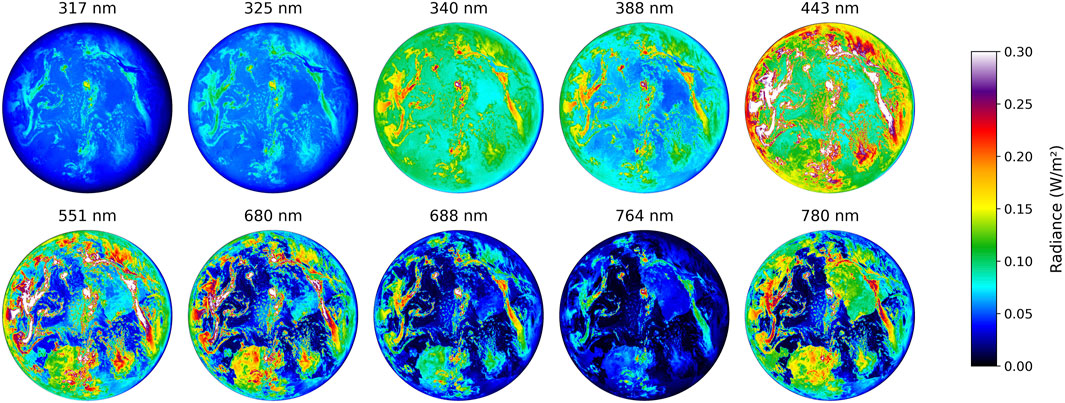
Figure 1. DSCOVR EPIC radiance imagery of the Earth taken at 14:47 UTC, 2016 August 7.

Despite the valuable insights gained from studying Earth as a proxy exoplanet, such approaches are inherently limited by our Earth-centric definition of life (Schwieterman et al., 2018). Consequently, researchers often focus on identifying unambiguous molecular or chemical signals that presuppose a fundamental degree of similarity between alien biochemistry and Terran biochemistry (Bartlett et al., 2022), with further contextual information (e.g., Kiang et al., 2018; Meadows et al., 2018). However, alien life may manifest in molecular or chemical forms distinct from those found on Earth (Bartlett and Wong, 2020). Even though, some fundamental physicochemical constraints may still apply universally. For instance, Vladilo and Hassanali (2018) argue that any biochemistry capable of sustaining life must involve extensive hydrogen bonding, which imposes thermal stability requirements broadly consistent with those observed for terrestrial life. These constraints suggest that while the molecular architecture of alien life may differ, its existence may still be confined to specific environmental conditions. In response, some researchers have proposed alternative and agnostic biosignatures (e.g., Dorn et al., 2011; Johnson et al., 2018; Marshall et al., 2021; Walker et al., 2018). In this sense, some agnostic approaches, which particularly emphasize 1) the complexity of molecular components (Dorn et al., 2011; Marshall et al., 2021) 2) the complexity of chemical reaction networks (Walker et al., 2018), and 3) planetary thermodynamic disequilibria (Krissansen-Totton et al., 2016; 2018; 2022), are motivated by the observation that the primary distinction between living and non-living systems lies in the capacity of life to utilize information to perform complex chemical and physical processes (Baluška and Levin, 2016; Davies and Walker, 2016; Farnsworth et al., 2013; Walker et al., 2016). Therefore, given that the complexity of the living world has generally increased over time, sometimes through striking major transitions, the greater the complexity and potentially the further from equilibrium a molecule or reaction network is observed to be, the higher the probability that it originates from a biotic process (Adami et al., 2000; Lineweaver et al., 2013; Smith and Szathmary, 1997).

Based on the ideas above, new perspectives on habitability propose that future works should instead focus on identifying systems that integrate sources of free energy, a variety of material constituents, and informational complexity (Wong et al., 2022), or alternatively, that habitability is fundamentally a manifestation of the existence of life (Chopra and Lineweaver, 2016; Lenardic and Seales, 2021). Additional approaches rooted in specific entropy metrics have also shown promise for assessing the potential habitability of exoplanets (e.g., Bartlett et al., 2022; Segal et al., 2024).

3 DSCOVR/EPIC

DSCOVR (formerly known as Triana⁴) was launched on 11 February 2015 and has been located at the first Sun-Earth Lagrange point (L1), approximately 1.5 million km from Earth since 8 June 2015. The collaborative mission between NASA (National Aeronautics and Space Administration), NOAA (National Oceanic and Atmospheric Administration), and the USAF (U.S. Air Force) primarily monitors space weather (e.g., solar winds), which is essential for ensuring the accuracy and lead time of NOAA’s space weather alerts and forecasts. It is also equipped with two NASA Earth-viewing instruments: the National Institute of Standards and Technology Advanced Radiometer (NISTAR⁵) and EPIC, which peer back at Earth and the entire planet to detect changes in the planet’s albedo, ozone absorption, and clouds (Herman et al., 2018). NISTAR is a cavity radiometer designed to measure the absolute and spectrally integrated irradiance that is reflected and emitted from the entire sunlit face of the Earth in three broad wavelengths as a single pixel. EPIC is an imager that provides global spectral images of the entire sunlit face of Earth with high spatial resolution (about 18 × 18 km², 10 wavelength bands).

The EPIC instrument consists of a 2048 × 2048 hafnium-coated charge-coupled device (CCD) camera with 12-bit readout electronics (Herman et al., 2018). The images are captured using 10 narrowband filters covering the ultraviolet (UV, 317.5, 325, 340, and 388 nm), visible (443, 551, 680, and 688 nm), and near-infrared (NIR, 764 and 779.5 nm) spectral ranges. Specifically, two of these channels (688 and 764 nm) are within the strongly absorbing oxygen B and A bands (Geogdzhayev and Marshak, 2018), respectively. Since 13 June 2015, EPIC has been capturing one full set of 10 wavelengths every 68–110 min, with exposure times ranging from 22 ms (551 nm) to 654 ms (317.5 nm). The camera has a 0.61° field of view (FOV) and a 1″07 angular sampling resolution and produces 2048 × 2048 images that are downsized to 1024 × 1024 pixels (except at 443 nm) with a nadir spatial resolution of about 18 km pixel^-1.The spectral characteristics of the 10 filters, including their bandwidths, peak transmissions, and quantum efficiencies, are summarized in Table 1 (Geogdzhayev and Marshak, 2018; Herman et al., 2018; Jiang et al., 2018).

Table 1

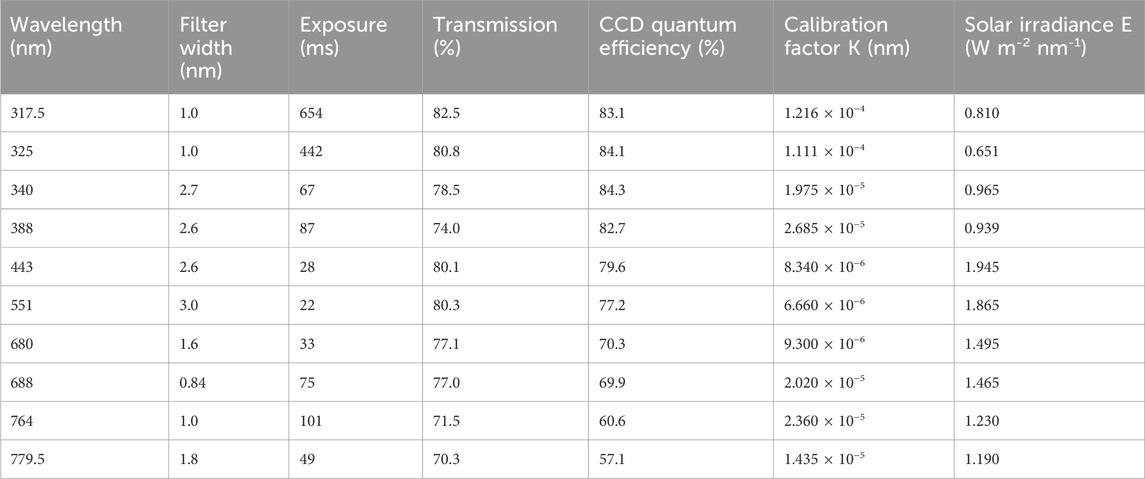
Table 1. Instrument parameters, calibration factors, and solar irradiance of EPIC wavelength band (adapted from Jiang et al. (2018)).

The EPIC Level 1B (L1B⁶) data are provided in engineering units of counts per second (counts s^-1), which are obtained by reading the CCD electronic signals through a 12-bit analog-to-digital (A/D) converter with a gain of 42 electrons per count and then dividing by the exposure time (Herman et al., 2018). The EPIC L1B images with the initial unit of counts per second (counts s^-1) were converted into reflectance (R) and radiance (I) through a calibration process (Jiang et al., 2018), and thus the EPIC radiance imagery of Earth was acquired (Figure 1).

While DSCOVR’s primary mission did not include exoplanet studies, its high-resolution Earth observations still provide a unique opportunity to construct disk-integrated rotational light curves of our planet. These time-resolved photometric measurements serve as an empirical reference for modeling Earth-like exoplanets that would appear as unresolved point sources in direct imaging observations (Jiang et al., 2018). Such datasets are particularly valuable for upcoming next-generation telescopes such as the ELT-PCS (Kasper et al., 2021), which will soon be capable of directly detecting and characterizing exoplanets within the habitable zones.

4 Observation of single-point Earth

4.1 Spectrum and frequency

Disk-integrated brightness of the sunlit portion of Earth (and occasionally the Moon) observed by EPIC serves as an ideal proxy for point-source measurements, analogous to observations of distant exoplanets (Jiang et al., 2018). The 388 nm radiance (Figure 1) is predominantly influenced by highly reflective clouds, with minimal contribution from the darker surface background, thus serving as an effective proxy for cloud distribution. In contrast, the 780 nm channel captures significant signals from both clouds and surface features. Fourier analysis using Lomb–Scargle periodograms (Lomb, 1976; Scargle, 1982; Hans et al., 1999) reveals distinct periodic signals in these channels, capturing the temporal variability driven by Earth’s rotation, orbital configuration, and the spatial distribution of clouds and surface features.

The qualitative results (Jiang et al., 2018) show that the variability of Earth’s light curve is largely influenced by the distribution of landmasses, oceans, and clouds. In the UV and visible bands, the reflected radiance is dominated by clouds and enhanced whenever clouds are present in the EPIC FOV. Surface contributions (i.e., positive landmass and negative ocean signals) are mixed with cloud signals in the visible wavelengths and become more prominent in the near-infrared channels. Earth appears brighter during the Southern Hemisphere (SH) summer due to its orbital eccentricity (∼0.017), which brings it closer to the Sun during that season. Additionally, the prominent feature in the Fourier spectra is the 24 h (1 day) peak (Figure 2), reflecting Earth’s 24 h rotation period. A few notable features with periods shorter than 24 h appear across all wavelengths at 12, 8, and 6 h, with the 12 h peak especially strong in the UV (Figures 2b,d). These signals likely result from periodic patterns of the Earth’s surface and cloud systems, which repeat daily when the Earth rotates. The period of 12 h could be a combined signature from clouds, oceans, and landmass patterns. For example, Asia and North America enter the FOV roughly 12 h apart in local time, and the Western Pacific faces EPIC around 02:00–03:00 UTC, followed by the Atlantic Ocean around 14:00–15:00 UTC. The 8-h and 6-h components may arise from the spatial variation of the cloud system and the continents, such as the ∼8 h difference between western Australia and northeastern Africa, and the ∼6 h interval between South America and southern Africa as they sequentially enter the EPIC FOV.

Figure 2

Time series and power spectrum plots. Panels (a) and (b) show the \(I_{388}\) time series and its power spectrum; (c) and (d) show \(I_{790}\) time series and power spectrum. Panels (e) and (f) illustrate PC1 time series and power spectrum; (g) and (h) depict PC2 time series and power spectrum. Each power spectrum features frequencies in days\(^{-1}\) on a logarithmic scale with power density, showing several peaks.

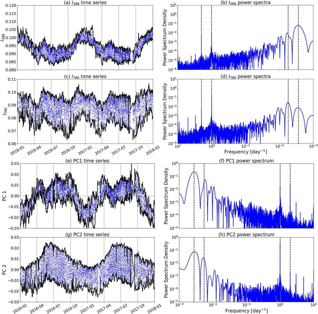
Figure 2. (a) Disk-averaged radiance spectra of I₃₈₈ from DSCOVR EPIC, with the envelopes of daily maxima and minima indicated by black lines. (b) Fourier power spectrum of the I₃₈₈ time series, with black dashed lines marking the frequencies corresponding to annual, semi-annual, diurnal, and semi-diurnal cycles. (c–f), as well as (g,h), follow the same format as (a,b), respectively, but correspond to I₇₈₀, PC1, and PC2. Panels (a–d) are modified from Fan et al. (2019) (e–h) are adapted from Fan et al. (2019). All panels are based on the same dataset as used in Figure 3 of Fan et al. (2019) and Figure 4 of Jiang et al. (2018).

4.2 Principal component and reflector

A quantitative analysis of the individual contributions from these components is essential for a comprehensive understanding of the light curve. While the spectral properties of known surface types can be estimated under different stellar spectral energy distributions (Shields et al., 2013), the specific surface composition of exoplanets remains unknown. Therefore, to maintain generality in the absence of such information, all types of land surfaces are treated as equivalent and represented with an “average” land surface (Fan et al., 2019). Acknowledging that future exoplanet observations may span different wavelength ranges, the reflectance time series is scaled to have zero mean and unit variance prior to further analysis. This normalization ensures equal weighting across spectral channels, which is particularly important for multivariate techniques such as singular value decomposition (SVD) and Gradient Boosted Regression Trees (GBRT; Friedman, 2001), which are sensitive to differences in data scale. The input dataset consisted of 10 reflectance channels along with 2 fractional coverage labels (land and cloud fraction, Figure 3) at each time step. In contrast, unnormalized reflectance values can be retained to preserve physical brightness information from different wavelengths. Additionally, EPIC Level 2 products, which are derived based on well-characterized properties of Earth (e.g., the distribution of surface types, the composition of the surface and atmosphere, and the spectral signatures of various spatial features), provide an opportunity to construct physically grounded models of planetary reflectance. The spatially resolved EPIC-view land cover (NASA/LARC/SD/ASDC 2017) and cloud data (NASA/LARC/SD/ASDC 2018), classified as the more specific fractional contributions of six distinct spatial features (i.e., ocean, desert, snow/ice, vegetation, and low and high clouds) were incorporated as additional indicators, resulting in a time series of 10 reflectance channels and 6 fractional coverage labels at each time step (Gu et al., 2021).

Figure 3

Line graph showing the relative importance of different elements across ten principal components (PC1 to PC10). Elements include low clouds, ocean, high clouds, vegetation, desert, snow/ice, and references from Fan et al., 2019.

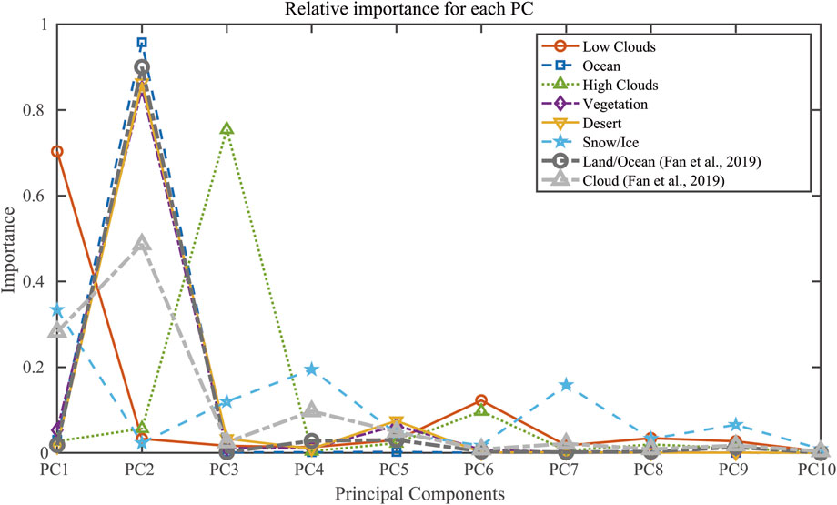
Figure 3. Relative importance of different spatial features for the first ten principal components. The line plot shows importance values (ranging from 0 to 1) of six spatial features: Low Clouds (orange), Ocean (blue), High Clouds (green), Vegetation (purple), Desert (golden yellow), and Snow/Ice (light blue). These values were derived from the Gradient Boosted Regression Trees (GBRT) model (modified from Gu et al. (2021)). The black and gray lines correspond to the Land/Ocean and Cloud model results reported by Fan et al. (2019), respectively; methodological details of the PCA and GBRT methods can be found in Section 3 of that work.

The GBRT results (Figure 3) as well as the eigenvalues of PCs (Figure 4a) suggest that PC1 and PC2 are the most important components with distinct contributions to land and cloud features, while the contributions from other PCs are relatively negligible (Figure 3; Fan et al., 2019). For land fraction, PC2 is dominant with a weight of 0.88, whereas PC1 contributes only 0.03. The variation in land/ocean fraction is thus primarily captured by PC2, showing a strong correlation of 0.91. Both PCs contribute substantially to cloud fraction, with weights of 0.28 for PC1 and 0.49 for PC2. The GBRT results also show that PC1 is strongly associated with low cloud, showing a flat spectral shape from UV to NIR wavelengths, consistent with cloud spectra, and a prominent peak corresponding to low clouds in observed data (∼70% relative importance) (Gu et al., 2021). The time series of PC1 is highly correlated with low cloud fraction (R = −0.8). PC2 captures information about land and ocean surfaces, with a spectrum that increases in reflectance with wavelength, matching their spectral behavior (Figure 4). GBRT shows peak importance for land/ocean labels (>84%), except for snow/ice, which may be due to its relatively low coverage on Earth’s surface (∼10%), confinement to high latitudes (resulting in smaller weight for disk integration), and/or slow temporal change. PC2 is strongly correlated with land/ocean contrast (R = −0.96). PC4 contains high cloud information, showing a flat spectrum with oxygen absorption features (688 and 764 nm). While GBRT indicates high cloud dominance (>71%), with a strong correlation (R = −0.82) between high cloud fraction and PC4, PC3 remains unclear but may relate to atmospheric Rayleigh scattering or ozone absorption due to its steep UV slope. PC5 shows peaks for vegetation/desert labels, suggesting it reflects the vegetation-desert contrast. Its spectrum (Figure 4b) is consistent with the VRE, and in experiments with only vegetation or desert, PC5 decreases significantly, providing weak evidence of its link to vegetation.

Figure 4

Graphical analysis of eigenvalues and principal component (PC) spectra. Panel (a) displays eigenvalue trends versus PC index with multiple color-coded lines representing different data sources: Fan et al. (2019), Gu et al. (2021, 2022) for observations and simulations. Panel (b) shows various PC spectra across wavelengths from 300 to 800 nm, with multiple line graphs indicating different PCs. Horizontal axes represent wavelength or PC index, while vertical axes indicate eigenvalue or spectral values. Various line styles and markers differentiate the data sources and PCs.

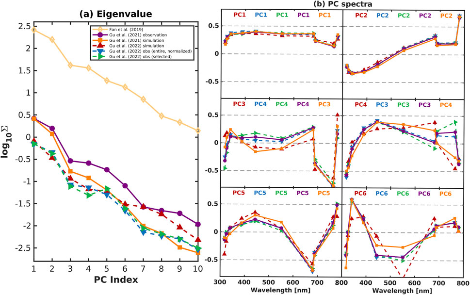
Figure 4. (a) Singular values (logarithmic scale) of principal components from multiple datasets: Fan et al. (2019) (orange diamonds), Gu et al. (2021) observations (red triangles) and synthetic data (blue inverted triangles), Gu et al. (2022) simulations (green right-pointing triangles), entire observations (purple circles), and selected observations (orange squares). Subsampling and normalization procedures follow the corresponding dataset specifications. (b) Eigenvectors of the first six principal components from the Gu et al. (2021) observations and simulations, and Gu et al. (2022) observations and simulations. To facilitate comparison, PC3 and PC4 are swapped between observations and simulations, following Gu et al. (2021), Gu et al. (2022). The legend in (b) corresponds exactly to that used in (a).

4.3 Surface mapping

Given the strong correlation between PC2 and surface features (Figure 3), and the comparable importance of PC1 and PC2 for clouds, it is inferred that clouds consist of two components: one independent of surface type, and the other associated with surface features. This interpretation aligns with previous studies that incorporate surface type into cloud albedo calculations (Thompson and Barron, 1981; Biasiotti et al., 2022). Specifically, PC2 exhibits smoother and more consistent daily changes (Figures 2g,h), while PC1 shows greater variability across days (Figures 2e,f). PC2 also tends to peak during summer, when the sunlit side of the Northern Hemisphere, with extensive landmass, is visible to both the Sun and the spacecraft. Its consistent diurnal variation likely reflects the combined effect of Earth’s rotation and the asymmetry in surface distribution, supporting the conclusion that the cloud variability is temporally correlated with surface features.

PC2 primarily captures the surface information about Earth with a strong linear correlation, thus making it possible to reconstruct a two-dimensional (2D) surface map. To facilitate generalization for future observations of Earth-like exoplanets, a set of simplified assumptions was adopted (Fan et al., 2019; Fan and Yung, 2020): the spectral properties of reflective surfaces were treated as unknown, the incoming solar flux was assumed to be uniform and known, and the entire planetary surface was modeled as a Lambertian reflector. Although Earth’s oceans are known to be strongly non-Lambertian, this assumption allows the method to be applied more broadly when surface characteristics are uncertain. The viewing geometry was assumed to be known and derived from DSCOVR navigation data over the 2-year observation period. Under these assumptions, the surface reconstruction becomes a linear regression problem (Fan et al., 2019). The reconstructed map (Figure 5a) shows PC2 values are positively correlated with land fraction. Coastlines are defined using the median PC2 value, aligning with the assumption that the total land coverage is unknown. Compared with the global land/ocean map of Earth (Figure 5b), the reconstructed map successfully captures all major continental features.

Figure 5

(a) Map showing 2D reconstruction with smooth color transitions ranging from red to blue, representing varying data values. (b) Global land/ocean map with distinct red for land and dark blue for ocean, illustrating geographical distribution. Both maps include color scales.

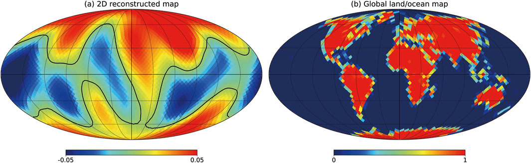
Figure 5. (a) Two-dimensional (2D) surface map of Earth, reconstructed using the time series of the PC2. The black contour line indicates the median value of PC2, which is used to represent coastlines. The regularization parameter of λ = 10⁻³ was used to construct the map. (b) Global land/ocean map of Earth for comparison (adapted figure from Fan et al. (2019)).

Building upon the framework (Fan et al., 2019; Fan and Yung, 2020), further studies have proposed enhancements to improve mapping fidelity and flexibility. Since global mapping is inherently ill-posed, Aizawa et al. (2020) applied sparse modeling techniques to improve the spatial resolution of inferred maps. Besides, Kawahara (2020) formulated a single inverse problem that unifies spin-orbit tomography and NMF (nonnegative matrix factorization)-based spectral unmixing, enabling the simultaneous retrieval of both spectral and geographical information from disk-integrated exoplanet light curves. Moreover, to account for temporal variability, Kawahara and Masuda (2020) developed a dynamic mapping approach by extending the Bayesian framework of Farr et al. (2018), utilizing analytical solutions to the Bayesian inverse problem with (multivariate) Gaussian priors and their isomorphic representations, thereby enabling the modeling of time-varying geography.

5 Numerical simulation

5.1 Reflecting surfaces

Since exoplanets will remain spatially unresolved point sources for the foreseeable future, quantifying the contribution of each spatial component to the integrated light curve is crucial for characterizing their habitability. Although PC2 is primarily interpreted (Fan et al., 2019) in terms of land and cloud fractions, Earth, as a well-observed and well-understood planet, provides a unique opportunity for more detailed modeling beyond such general correlations. Leveraging the availability of high-resolution data on Earth’s surface composition and atmospheric constituents, it becomes feasible to simulate its reflective signatures through physical models that account for diverse surface types, cloud structures, and atmospheric scattering effects.

As discussed above, the EPIC Level 2 products provide the opportunity to clarify 6 spatial features. By using a two-dimensional moving average applied to the pixel-level reflectance data within the phase space defined by the solar and viewing zenith angles, the reflected intensity for each spatial feature at a given wavelength is calculated. This enables the construction of a temporally varying Earth image model, which can then be used to reconstruct DSCOVR observations, analyze their relationship with the spatial features, and interpret the physical meaning of the principal components (Gu et al., 2021).

Assumed that the entire sunlit disk is uniformly covered by each of the six spatial features individually, the corresponding disk-averaged reflection spectra for a synthetic Earth (Figures 6a,b) provides characteristic spectral profiles associated with reflecting surfaces (Gu et al., 2021). For each time step, the reflectance contribution of a given spatial feature was calculated by dividing its total reflectance by the disk-integrated reflectance and a daily average of these contributions was then applied (Figure 6c). The slopes in the first three UV channels result from Rayleigh scattering and ozone absorption. Absorption features from the oxygen A and B bands at 764 nm and 688 nm influence the spectral shape, leading to minimal spectral differences among spatial features. Oxygen absorption is weaker in high clouds compared to low clouds (or the surface) due to shorter optical path lengths, suggesting the possibility of distinguishing high and low clouds in the disk-integrated spectrum. The spectral shape of ice/snow reflectance closely matches that of low clouds, making it difficult to identify their contribution to individual light curves due to smaller coverage. Vegetation is the only feature showing a monotonic increase in reflectance at the longest wavelengths, consistent with the VRE (i.e., 680, 688, and 764 nm). In the first four UV channels (Figure 6c), ocean and cloud contributions dominate (around 40%), with atmospheric scattering and ozone absorption influencing the reflectance (Jiang et al., 2018), making it hard to distinguish surface features. At longer wavelengths, low clouds contribute up to ∼60%, while high clouds are more significant at 688 and 764 nm due to stronger oxygen absorption in the lower atmosphere. Vegetation shows higher contributions in the NIR channels, consistent with the VRE. The seasonal cycle, with more vegetation and less ocean in the northern summer, is also apparent in the time series.

Figure 6

Charts of reflectance data across different wavelengths from 300 to 800 nm. (a) Shows disk-integrated reflectance spectra with varying patterns for vegetation, desert, snow/ice, ocean, high clouds, low clouds, and Earth mean. (b) Displays spectral deviation from Earth mean. (c) Depicts temporal contributions for different wavelengths, highlighting proportions of ocean, desert, vegetation, snow/ice, high clouds, and low clouds over months.

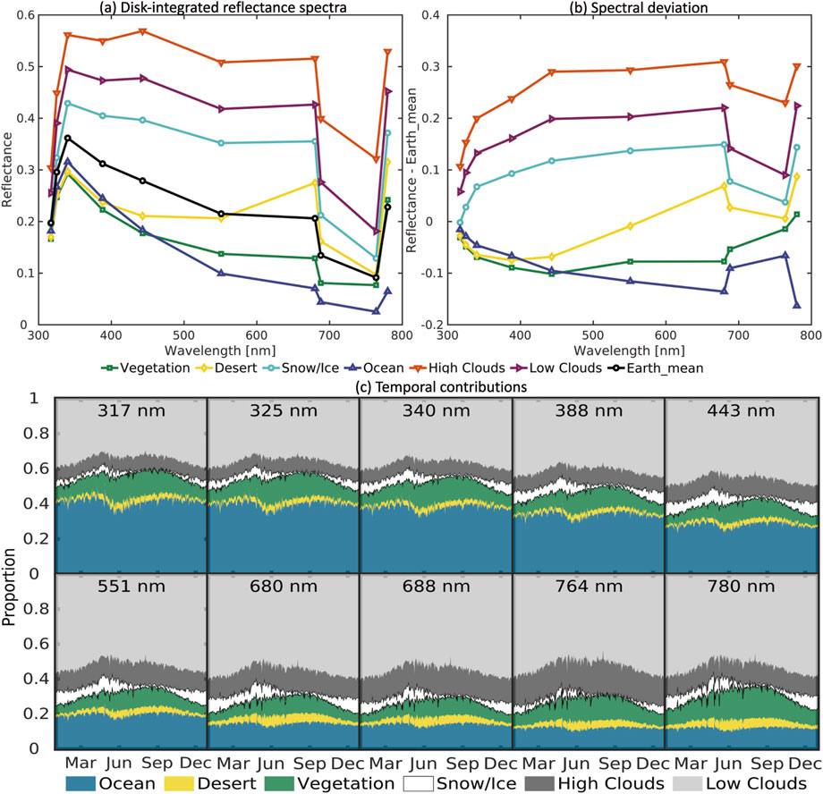
Figure 6. (a) Disk-integrated, full-phase reflection spectra of six spatial features (colored lines) compared with that of the globally averaged Earth (black line). (b) Spectral differences between each spatial feature and the global average, based on (a). (c) Daily averaged time series of fractional reflectance contributions from the six spatial features (adapted from Gu et al. (2021)).

The eigenvalues (Figure 4a) of PC1 and PC2 indicate that they together explain over ∼97% of the total variance, with values nearly an order of magnitude larger than that of PC3 (Gu et al., 2021). PC3–6 form a secondary group, potentially capturing weaker yet meaningful spatial signals. Components beyond PC6, each contributing less than ∼0.02% of the variance, are treated as noise and excluded from further analysis. Despite slightly lower eigenvalues, the synthetic single-point light curves successfully reproduce all characteristic spectral features, except for minor switching between the observed and reconstructed eigenvectors for PC3 and PC4 (Figure 4b). The result is promising, especially considering that the reconstruction was achieved using only six spatially distinct yet temporally invariant surface and atmospheric components.

5.2 Atmosphere

Although a non–radiative transfer (non-RT) Earth model was employed (Gu et al., 2021) and successfully demonstrated that information related to low clouds, surface type distribution, and high clouds is encoded in different PCs of Earth’s light curves, the absence of radiative transfer processes in such models still limited their ability to assess the influence of atmospheric composition and scattering. Previous studies (e.g., Tinetti et al., 2006a; Tinetti et al., 2006b; Robinson et al., 2011; Feng et al., 2018; Batalha et al., 2019) have attempted to model Earth’s light curves using RT models, yet these efforts lack validation against observations extending beyond a few days. Consequently, the development of a comprehensive RT model of Earth, rigorously tested against long-term and diverse observations, remains both critical and pressing.

To investigate the influence of atmospheric radiative transfer on Earth’s disk-integrated reflectance, the Earth Spectrum Simulator (ESS) is developed (Gu et al., 2022). The ESS model incorporates the two-stream-exact-single-scattering (2S-ESS) line-by-line RT model that combines precise single-scattering calculations with a two-stream approximation for multiple scattering and offers a balance between computational efficiency and accuracy (Spurr and Natraj, 2011) and has been widely applied in Earth remote sensing of greenhouse gases and aerosols (Xi et al., 2015; Zhang et al., 2015; 2016; Zeng et al., 2017; 2018; Huang et al., 2020; Natraj et al., 2021), thus accounting for surface reflection, cloud and aerosol scattering, and gaseous absorption.

In the 2S-ESS model, surface reflectance was simulated through BRDFs (Bidirectional Reflectance Distribution Functions, Figure 7a), and then land surfaces were categorized into seven types (NASA/LARC/SD/ASDC, 2017). For snow- and ice-covered pixels, a Lambertian surface albedo was assumed. Additionally, the Rayleigh scattering and molecular absorption were simulated considering only the influence of O₂, H₂O, and O₃, due to their dominant influence in the narrow spectral bands of EPIC. The vertical water vapor and temperature were assumed spatially invariant while surface pressure varied spatially and temporally. The surface pressure (Figure 7c) data was derived from MERRA-2 (Modern-Era Retrospective analysis for Research and Application, Version 2). The 3D ozone distributions were derived (Figure 7d), and all atmospheric fields were sampled on the 5th, 15th, and 25th days of each month to reduce computational demands. Aerosol optical properties (Figure 7e) were calculated using Mie scattering theory, except for dust, where nonsphericity is considered (Meng et al., 2010; Crisp et al., 2021). Clouds (Figure 7f) were further classified as either liquid or ice, with one type per pixel and fixed vertical distributions and their optical properties were based on Mie theory (Hess et al., 1998) for liquid clouds and a cirrus habit mixture (Baum et al., 2011) for ice clouds. For pixels with mixed cloud types at degraded resolution, multiple RT simulations were performed and averaged based on cloud fraction to obtain the final reflectance.

Figure 7

Six globe images demonstrate different environmental data: (a) Land cover with diverse colors indicating vegetation density. (b) Ocean productivity with gradients in color. (c) Surface pressure displaying intense reds. (d) Ozone levels with variations across regions. (e) Aerosol distribution in vivid patterns. (f) Cloud cover with intricate textures. Each image includes a color bar legend on the side.

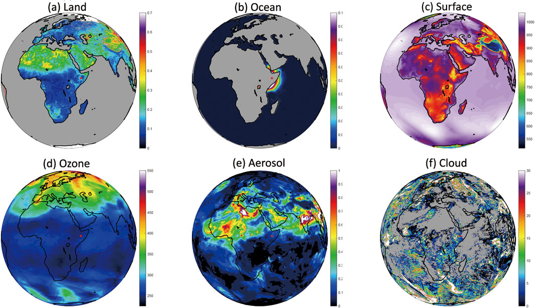
Figure 7. (a) Land reflectance map calculated using the Ross–Thick–Li–Sparse model (Roujean et al., 1992). Model coefficients for the 443, 551, 680, and 780 nm channels were obtained from the DSCOVR MAIAC Version 02 dataset (NASA/LARC/SD/ASDC, 2018) and the viewing geometry information is provided by the EPIC Level 1B dataset (NASA/LARC/SD/ASDC, DSCOVR EPIC Level 1B Version 3). (b) Ocean reflectance map from the Cox–Munk model (Cox and Munk, 1954). (c) Surface pressure map from MERRA-2 reanalysis (Global Modeling and Assimilation Office, 2015b). (d) Column-integrated ozone map generated following the approach described in Crisp et al. (2021). (e) Total aerosol optical depth. The mixing ratios of dust, sulfate, sea salt, black carbon, and organic carbon are extracted from MERRA-2 (Global Modeling and Assimilation Office, 2015a). (f) Total cloud optical depth. Cloud optical depth, effective pressure, and effective radius (for ice clouds) are obtained from EPIC composite data (NASA/LARC/SD/ASDC, 2017) (adapted from Gu et al. (2022)).

Generally, the ESS can reproduce the major features observed accurately. In the shortest wavelength channels, strong Rayleigh scattering results in generally bright images, with the 340 nm channel being the brightest (Figure 8), which is consistent with the brightness variations caused by the enhanced ozone absorption between 340 nm and 317 nm. In the longer wavelength channels, surface information becomes more clearly visible, except for the two oxygen absorption channels (688 nm and 764 nm). In particular, due to the VRE, the reflectance of vegetated pixels increases significantly in the 780 nm channel, forming a sharp contrast with desert pixels, whose reflectance gradually increases across the 551 nm, 680 nm, and 780 nm channels. These spectral differences among different surface types benefit from the detailed modeling of land surface BRDF. In terms of atmospheric scattering features, the use of MAIAC data enables effective simulation of the backscattering peak observed under EPIC viewing geometry; meanwhile, the adoption of the Cox–Munk surface model allows the simulation to capture the feature of ocean glint (Figure 7b).

Figure 8

Ten global maps displaying various intensity levels at different nanometers (317nm to 780nm) using a color scale. The scale ranges from blue (low intensity) to red (high intensity), representing data over the Earth's surface, particularly over oceans and landmasses.

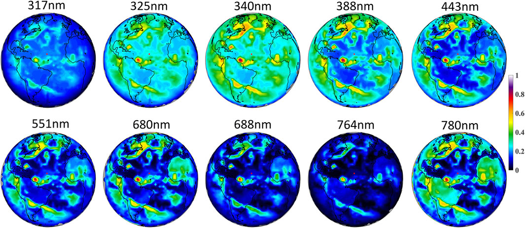
Figure 8. EPIC synthetic reflectance images in 10 channels at 14:47 UTC, 2016 August 7 (adapted from Gu et al. (2022)).

Specifically, the ESS model successfully reproduces the time-averaged spectra with errors generally below 5%, and within 7% overall, except at the two oxygen absorption bands (688 nm and 764 nm), where simulated reflectance exceeds observations by up to 19.53%. The model exhibits slightly larger temporal variability than observations. In the 317–443 nm range, the simulated reflectance tends to be slightly darker than observed, while simulations at longer wavelengths generally appear brighter. A pronounced seasonal cycle is captured in the Southern Hemisphere, with higher reflectance during summer, likely due to the closer Earth–Sun distance and the presence of the Antarctic ice sheet. A smaller enhancement is also observed in the Northern Hemisphere summer, which may be attributed to increased land surface reflectance and cloud cover driven by the South Asian monsoon (Jiang et al., 2018).

The comparison between the simulated and observed PCs (Figure 4) includes an additional subsampled dataset of approximately 300 time points, selected to align with the simulation output. This subset captures the main temporal variability of the light curves, as indicated by the relatively small amplitudes of higher-order singular values (Figure 4a; Gu et al., 2021). At the same time points, the singular values from the simulations are generally larger than those from the observations, suggesting stronger temporal variability in the simulated light curves. Notably, PC3 and PC4 appear to be interchanged between the simulation and observation (Figure 4b). The simulation successfully reconstructs PC1-5; in particular, the first two PCs show near-perfect agreement, demonstrating that the ESS model accurately reproduces the two most dominant signals, namely, low cloud and surface reflectance patterns, which is in line with the previous findings (Gu et al., 2021). The observed PC4 and PC3 also correspond well to the simulated PC3 and PC4, respectively. Since observed PC4 is primarily associated with high clouds (Gu et al., 2021), and ESS tends to simulate higher reflectance for high clouds, the corresponding eigenvalue increases due to the enhanced variance contribution from high cloud coverage.

Although the details of cloud features show some differences, mainly because the simulation uses the DSCOVR composite cloud dataset, which does not exactly match the instantaneous cloud distribution observed by EPIC, the ESS model still serves as a valuable tool for generating light curves of Earth-like exoplanets and provides an important platform for combining with global climate models (GCMs) to support exoplanet characterization studies with its high fidelity, robustness, and efficiency.

6 Habitability metric

6.1 Complexity

In the context of measuring exoplanet complexity, two key aspects must be considered: 1) how to formally quantify complexity, and 2) how to use remotely detectable signals to assess the complexity of a given exoplanet. To address the first, the formal epsilon machine (EM) framework has been in development for several decades (Crutchfield, 2012), and was applied to the challenge of exoplanet characterization (Bartlett et al., 2022). EMs are discrete mathematical objects (finite state machines) that can compactly represent both simple random and simple deterministic processes (as contrasted with minimal Turing machine programs, which ascribe high complexities to simple random processes). They also have the capacity to reveal the underlying phase-space structure of nonlinear systems (Brodu, 2011; Packard et al., 1980; Crutchfield et al., 1986). EMs are particularly well suited to the analysis of planetary light curves, as they are designed to fulfill several key criteria: 1) reproduce deterministic features of the input time series; 2) reproduce random stochastic features of the input time series; 3) serve as the optimal predictor of the generating process; and 4) represent the internal structure of the generating process in the most compact form (Brodu, 2011; Crutchfield, 2012). These kinds of algorithms take a time series as input and produce a minimal optimized model (the EM) capable of reproducing time series that are, subject to parameter tuning and data quality, etc., statistically equivalent to the original. The size of the resulting model, particularly the information content of its state-space distribution, defines a metric known as statistical complexity.

To address the second challenge, it is hypothesized that planets exhibiting the highest complexity are the most likely to host biospheres, with Earth serving as the initial reference. Even if lifeless planets with high complexity are identified, the approach remains valuable as a characterization tool, given the largely unknown space of exoplanet types, which could vary widely in complexity. For example, the Moon exhibits very low complexity, while the Sun and Jupiter display somewhat richer structures and variability. Earth, with its active atmosphere, hydrosphere, and biosphere, appears to be the most complex body in the Solar System (Kasting and Siefert, 2002; Dyke et al., 2011; Olejarz et al., 2021), although this has yet to be quantitatively confirmed. By using EMs derived from reflectance time series, exoplanet complexity levels can be estimated, which could serve as a potential biosignature.

6.2 Shannon entropy

As an initial statistical assessment, the Shannon entropy was calculated for each proxy exoplanet reflectance time series (Bartlett et al., 2022). The reflectance values were discretized and normalized, and the entropies were computed using the standard formula based on the frequency of occurrence for each reflectance value. These entropies were then averaged over the ten EPIC wavelength channels. On the complexity-entropy plane (Figure 9a), groups are observed along a monotonic slope of increasing complexity and entropy despite inherent noise and data sampling issues. The simplest synthetic Earths (cloudless, mono-surface worlds) exhibit the smallest Shannon entropy, while the highest entropy is observed in the most qualitatively and quantitatively complex case (the original Earth). Within the cloudy worlds, there is a relatively small distinction between the mono-surface and multi-surface groups, but it is promising to observe any distinction despite the cloud cover’s masking effect.

Figure 9

Four scatter plots labeled (a), (b), (c), and (d) display variations in statistical complexity versus entropy metrics. Panel (a) compares Shannon entropy to statistical complexity across different environments and conditions, denoted by various shapes and colors. Panel (b) illustrates Shannon entropy against statistical complexity for Earth and Jupiter at different wavelengths. Panel (c) shows average differential entropy versus average statistical complexity, with distinctions in surface types and cloud presence. Panel (d) plots joint differential entropy of eigencolors versus average statistical complexity, with markers representing diverse environmental conditions and cloud statuses.

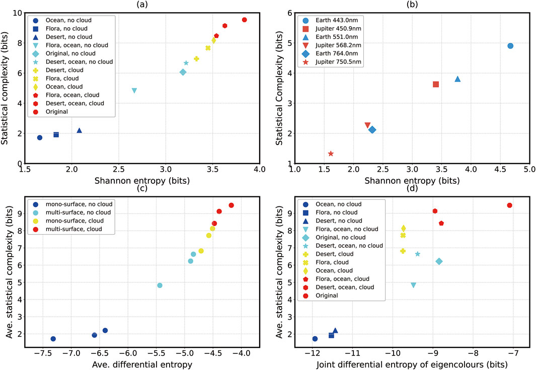
Figure 9. (a) Statistical complexity versus Shannon entropy averaged across all wavelength bands for the original and synthetic Earth data, as analyzed in Bartlett et al. (2022) (b) Complexity–entropy comparison between Earth and Jupiter time series after processing. The Jupiter datasets were obtained from the Cassini mission, which collected data over approximately 44 Earth days (∼107 Jupiter days) across nine wavelength channels. Three of these channels were selected for comparison with Earth data: (1) 443 nm (Earth) and 450.9 nm (Jupiter), (2) 551 nm (Earth) and 568.2 nm (Jupiter), and (3) 764 nm (Earth) and 750.5 nm (Jupiter). (c) Statistical complexity versus differential entropy. Consistent with the findings of Bartlett et al. (2022), cloudy worlds exhibit the highest values. A relatively small distinction is observed between the mono-surface and multi-surface groups within the cloudy category. (d) Statistical complexity as a function of joint differential entropy of eigencolors. (a,b) are modified from Bartlett et al. (2022), and (c,d) are modified from Segal et al. (2024).

To further explore the potential for distinguishing living from non-living planets, the gas giant, Jupiter, which is generally assumed to be sterile and known for its complex atmosphere that exhibits both periodic and stochastic features, was compared with Earth (Bartlett et al., 2022; Figure 9b). For each wavelength considered, Earth exhibited higher complexity and entropy than Jupiter, with an average difference of approximately 1.25 bits for complexity and 1 bit for entropy, although these values vary depending on the wavelength. Even though the lower image resolution of the Cassini data may have affected the information content of the Jupiter data, these results still suggest that Earth’s planetary complexity exceeds that of Jupiter, which is consistent with the hypothesis that planetary complexity correlates with the presence of life. However, further investigation is required to fully understand the causal influences leading to this observed correlation.

6.3 Joint differential entropy

When analyzing an object using discrete data, it’s possible that important details in the original measurements are lost during the discretization (binning) step. In contrast, methods applicable to continuous time series data may reveal important, perhaps subtle features that could aid in planetary characterization. This was the motivation for Segal et al. (2024) to employ an approximation for the entropy of a continuous variable to DSCOVR EPIC reflectance time series. Specifically, they used the Vasicek estimate of the differential entropy (Vasicek, 1976). PCA applied to the spatially unresolved multiwavelength reflectance data for each synthetic Earth used by Bartlett et al. (2022) and the average differential entropy (Figure 9c) was derived. This was found to be approximately proportional to the joint differential entropy (JDE). Figure 9d shows that the average JDE of eigencolors, obtained via PCA, reveals a new level of distinctions between the synthetic Earth time series data. Unlike the original wavelength channels, eigenvectors are linearly independent which means that cross-wavelength mutual information, such as that introduced by cloud cover, is only accounted for once (Segal et al., 2024). This is supported by the average Pearson correlation coefficient among the 10 eigencolors, which is on the order of 10^–17 for both Earth and the reconstructed worlds. In contrast, when the correlation is computed across the original EPIC narrow band wavelengths, the average value is approximately R = 0.57 for the original Earth data and decreases to R = 0.08 for the cloud-removed version. These results are consistent with previous findings that reflectance variability due to clouds is across all 10 EPIC bands (Jiang et al., 2018).

7 Summary

This paper presents recent milestones in studying Earth as a proxy for habitable exoplanets, utilizing single-point, multi-spectral data from the DSCOVR/EPIC instrument. By integrating observations across ultraviolet, visible, and near-infrared bands, these measurements provide essential insights into the temporal and spectral variability of Earth’s disk-integrated reflectance. Such information is crucial for guiding the interpretation of remote sensing data from spatially unresolved observations of terrestrial exoplanets.

Earth’s photometric signature, when treated as that of a distant point source, captures significant diurnal and seasonal variations. These variations are shaped by the dynamics of atmospheric and surface features. Initial analyses demonstrated that averaging EPIC’s full-disk images could replicate the observational constraints expected in exoplanet missions. Temporal analysis techniques revealed periodic signals tied to planetary rotation, cloud cover, and surface distribution. To extract meaningful structure from these light curves, principal component analysis was employed to identify dominant modes of variability. The leading principal components captured distinct physical processes, including cloud dynamics and land-ocean contrast. These results enabled the reconstruction of a simplified surface map of Earth without predefined surface information, offering a method adaptable to diverse planetary systems.

Further investigations introduced physically based models that quantified the individual roles of atmospheric layers and surface types. The influence of low clouds proved especially strong in the ultraviolet and visible bands, while contributions from vegetation, high-altitude clouds, and oceans became more prominent at longer wavelengths. These studies clarified how different components contribute to the overall photometric signal. To simulate Earth’s reflectance with greater fidelity, a radiative transfer model was developed through the Earth Spectrum Simulator. This tool incorporated surface reflectance properties, atmospheric scattering, and absorption processes and its simulations closely matched observations, providing strong validation of the model’s accuracy and its capacity to replicate key spectral and temporal patterns.

Beyond chemical heuristics for biosignature detection, new methodologies based on information theory and complexity science were described, which offer new means to assess exoplanets and agnostically search for life. These approaches revealed that Earth’s reflectance time series displays significantly higher complexity than our gas giant companion (Jupiter). This complexity is proposed as a potential agnostic biosignature, reflecting dynamic processes that could be causally linked to biological activity.

The combined use of observational analysis, physical modeling, and complexity metrics forms a comprehensive framework for characterizing terrestrial exoplanets, integrating various scientific disciplines to enhance our understanding of diverse planetary systems. By leveraging high-resolution multi-spectral observations, physical models, and advanced techniques for assessing complexity, this research not only refines our ability to study exoplanetary environments but also contributes to the development of diagnostic tools for evaluating habitability and signs of life.

Author contributions

XJ: Writing – review and editing, Writing – original draft. LG: Writing – review and editing, Methodology. SF: Project administration, Writing – review and editing, Methodology. SJB: Methodology, Writing – review and editing. JY: Writing – review and editing. JHJ: Writing – review and editing, Conceptualization. YL: Validation, Writing – review and editing. YY: Supervision, Writing – review and editing.

Funding

The author(s) declare that financial support was received for the research and/or publication of this article. SF acknowledges funding from the Stable Support Plan Program for the Higher Education Institutions of the Shenzhen Science and Technology Innovation Commission through grant No. 20231115103030002. JHJ acknowledged the support from the Jet Propulsion Laboratory, California Institute of Technology, sponsored by NASA. JHJ and SJB acknowledge support from the NASA XRP (Exoplanets Research Program) grant no. 22-XRP22_2-0044.

Conflict of interest

The authors declare that the research was conducted in the absence of any commercial or financial relationships that could be construed as a potential conflict of interest.

Generative AI statement

The author(s) declare that no Generative AI was used in the creation of this manuscript.

Publisher’s note

All claims expressed in this article are solely those of the authors and do not necessarily represent those of their affiliated organizations, or those of the publisher, the editors and the reviewers. Any product that may be evaluated in this article, or claim that may be made by its manufacturer, is not guaranteed or endorsed by the publisher.

Footnotes

¹https://exoplanetarchive.ipac.caltech.edu/

²https://science.nasa.gov/astrophysics/programs/habitable-worlds-observatory/

³http://epic.gsfc.nasa.gov

⁴http://www.nesdis.noaa.gov/DSCOVR/

⁵http://www.nesdis.noaa.gov/DSCOVR/spacecraft.html

⁶https://eosweb.larc.nasa.gov/project/dscovr/dscovr_table/

References

Adami, C., Ofria, C., and Collier, T. C. (2000). Evolution of biological complexity. Proc. Natl. Acad. Sci. 97 (9), 4463–4468. doi:10.1073/pnas.97.9.4463

PubMed Abstract | CrossRef Full Text | Google Scholar

Aizawa, M., Kawahara, H., and Fan, S. (2020). Global mapping of an exo-Earth using sparse modeling. Astrophysical J. 896 (1), 22. doi:10.3847/1538-4357/ab8d30