Multi-Scale graph wavelet convolutional network for hyperspectral image classification

Hyperspectral images (HSIs) have very high dimensionality and typically lack sufficient labeled samples, which significantly challenges their processing and analysis. These challenges contribute to the dimensionality curse, making it difficult to describe complex spatial relationships, especially those with non-Euclidean characteristics. This paper presents a multi-scale graph wavelet convolutional network (MS-GWCN) that utilizes a graph wavelet transform within a multi-scale learning framework to accurately capture spatial-spectral features. The MS-GWCN constructs graphs according to 8-neighborhood connectivity schemes, implements spectral graph wavelet transforms for multi-scale decomposition, and aggregates features through multi-scale graph convolutional layers. Our method, the MS-GWCN, demonstrates superior performance compared to existing methodologies. It achieves higher overall accuracy, average accuracy, per-class accuracy, and the Kappa coefficient, as evaluated on three datasets, including the Indian Pines, Salinas, and Pavia University datasets, thereby demonstrating enhanced robustness and generalization capability.

1 Introduction

Hyperspectral images (HSIs) have become a cornerstone of modern remote sensing by capturing detailed spatial and spectral information across hundreds of continuous bands. This capability enables precise material discrimination in applications ranging from environmental monitoring and precision agriculture to military reconnaissance (Kipf and Welling, 2016). Despite these advantages, HSIs’ high dimensionality causes the Hughes phenomenon, where sample sparsity reduces classification accuracy as spectral bands increase. Additionally, the limited availability of labeled training samples in many remote-sensing scenarios exacerbates these issues, making robust model training difficult (Ma et al., 2013; Hughes, 1968). Traditional machine learning approaches, such as support vector machines (SVM) (Melgani and Bruzzone, 2004) and random forests (RF) (Zhang and Ma, 2012), have been widely adopted to address HSI classification. These methods primarily focus on spectral-feature analysis, often employing linear dimensionality-reduction techniques (e.g., principal component analysis, PCA) to mitigate redundancy. However, PCA and similar projections can inadvertently discard essential nonlinear spectral cues to distinguish spectrally similar classes (e.g., grassland vs. shrubs) (Uddin et al., 2020). Moreover, these conventional algorithms overlook the inherently non-Euclidean spatial relationships between pixels, which carry critical contextual information, especially in complex terrains, where adjacent pixels exhibit strong dependencies that facilitate class separation (Kang et al., 2014).

Emerging deep neural architectures have aimed to integrate spectral and spatial features within a unified framework to address these shortcomings. Three-dimensional convolutional neural networks (3D-CNNs) extend standard CNNs into the spectral domain, learning hierarchical spatial-spectral representations directly from the HSI cube (Li et al., 2017). Although 3D-CNNs enhance the discrimination of subtle spectral differences, their heavy computational burden and large parameter counts often limit practical deployment. Convolutional bidirectional long short-term memory networks (Conv-BiLSTMs) treat the spectral bands as a sequence, modeling dependencies along the spectral dimension while preserving spatial context; this approach improves performance in label-scarce settings but still relies on grid-based convolutions that cannot naturally adapt to irregular spatial structures (Liu et al., 2017).

Graph neural networks (GNNs) have emerged as a powerful alternative, where each pixel is represented as a node and spatial-spectral affinities are encoded as edges. Spectral–Spatial Graph Convolutional Networks (SS-GCNs) construct adjacency matrices using k-nearest neighbors (k-NN) in spectral feature space, enabling graph convolutions to operate on non-Euclidean data (Cao and Messinger, 2025). Although SS-GCNs excel in small, homogeneous scenes, their fixed-graph nature often misrepresents long-range dependencies in heterogeneous land cover, leading to performance degradation. Adaptive Graph Attention Networks (AGAT) enhance flexibility by learning edge weights dynamically based on feature correlations. However, their single-scale aggregation still suffers from over-smoothing in regions with multi-resolution textures (Yang JY. et al., 2022).

Dual-stream GCNs attempt to address spectral-spatial decoupling by processing spectral and spatial features in parallel branches before late fusion; however, this separation limits cross-modality interactions during message passing, particularly along boundaries where spectral diversity and spatial fragmentation coexist, resulting in significant accuracy drops in wetland classification tasks (He X. et al., 2022). Hierarchical graph pyramid networks introduce multi-scale pooling to capture coarse-to-fine features (Liu et al., 2024), while multi-resolution graph convolution frameworks aggregate information from graphs built at various neighborhood scales (Wan et al., 2020). However, both approaches rely on manually chosen pooling ratios or dilation factors, which restrict adaptability across diverse scenes.

To address these limitations, dynamic GCN variants have been developed. Ding et al. (2022) proposed a dynamic adaptive sampling GCN that captures neighborhood information through learnable sampling strategies. Concurrently, Yang B. et al. (2022) designed a deep adaptive graph integration network to dynamically optimize graph configurations. Yu et al. (2023) enhanced contextual modeling through a dual interactive GCN mechanism. Hybrid approaches that combine GCNs with CNNs (Liu et al., 2021; Dong et al., 2022) generate complementary spectral-spatial features; however, challenges such as computational inefficiency in high-dimensional graph processing, isotropic aggregation, and multi-scale representation bottlenecks persist (Ding et al., 2024). Multiresolution graph signal processing (MGSP) offers a principled solution by utilizing spectral graph wavelet transforms (SGWTs) to decompose signals into scale-specific components, thereby capturing both fine boundary details and broader contextual trends (Ander et al.). Chebyshev polynomial approximations enhance SGWTs by circumventing explicit eigen-decomposition, reducing computational costs (Cai et al., 2023). Nevertheless, existing MGSP-based methods rely on static scales and fixed topologies, failing to align with scene-specific spectral-spatial interactions or mitigate atmospheric artifacts (Behmanesh et al., 2024).

Recent works emphasize structural priors for HSI. PFS3F integrates multiscale superpixel-wise spatial cues—refined via extended random walk (ERW)—with semantic-aware structural features in a probabilistic fusion framework, demonstrating the benefit of combining segmentation granularity and semantic structure. From Global to Local further adopts a dual-branch scheme: global structures are extracted by pyramid texture filtering while local structures are captured with multiscale superpixels, and the resulting probabilities are fused for classification. Complementary to these image-domain, handcrafted pipelines, Contour Structural Profiles (CSP) introduces an edge-aware descriptor to alleviate over-smoothing and enhance boundary consistency (Zhang et al., 2025a; Zhang et al., 2025b; Zhang et al., 2022).

Different from the above, our MS-GWCN performs end-to-end learning in the graph spectral domain, where multi-scale graph wavelet convolutions unify local–global modeling and provide band-pass control to preserve edges while avoiding excessive smoothing; this yields a compact pipeline that reduces manual feature engineering and naturally accommodates graph constructions (e.g., pixel- or superpixel-based adjacency).The proposed MS-GWCN introduces a novel method for HSI classification by embedding multi-scale wavelet transforms within a graph-based convolutional framework. Leveraging the spectral decomposition of the normalized Laplacian, we apply wavelet filters at multiple scales to extract hierarchical features that simultaneously capture fine-grained, high-frequency pixel details and broader, low-frequency regional contexts. We construct the graph using an 8-neighborhood connectivity model on normalized 2D feature maps to preserve spatial coherence. These multi-scale wavelet responses are integrated through trainable graph convolutional filters and non-linear activations, enabling frequency-aware feature aggregation that adapts to the underlying spectral-spatial structure. As demonstrated in Figure 1, by combining multi-scale graph wavelet transforms with deep neural layers, MS-GWCN proceeds through three clear phases: graph construction from HSI cubes, dyadic wavelet decomposition into scale subspaces, and attention-guided fusion of wavelet coefficients via graph convolutions, culminating in a fully connected layer that produces robust class probability estimates. The adaptability of MS-GWCN across diverse scenes provides reassurance about its potential in HSI classification.

Figure 1

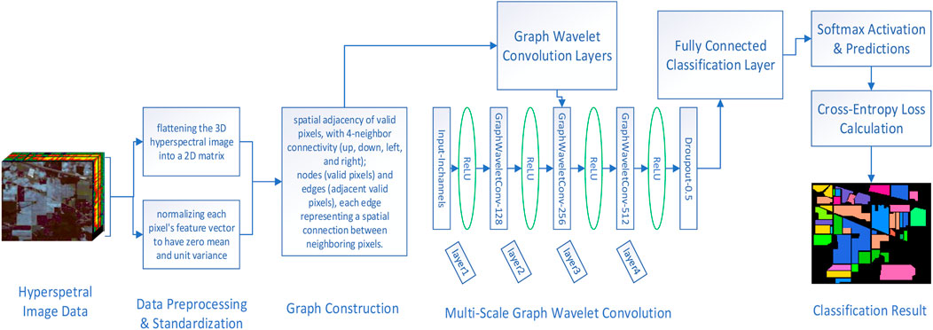
Figure 1. The framework of our MS-GWCN algorithm.

The diagram of Figure 1 illustrates the significant stages of the proposed method: (1) graph construction from the input HSI (each pixel is treated as a graph node, and edges connect 8-neighborhood adjacent pixels), preserving the spatial relationships; (2) multi-scale graph wavelet decomposition, where spectral graph wavelet transforms at multiple scales extract features corresponding to different frequency components (from fine to coarse); (3) graph convolution and feature aggregation across scales, including an attention-based fusion of the multi-scale features; and (4) a final classification layer that predicts the land-cover class for each pixel. The legend in the figure clarifies the symbols used for graph nodes, wavelet filters at various scales, convolution operations, and the attention mechanism for scale fusion.

The contributions of our work can be summarized as follows.

1. Extraction of multi-scale features from HSI is essential for accurately capturing spectral-spatial and contextual elements, which are crucial for HSI classification. The graph wavelet transforms operate across various scales, enabling the extraction of extensive hierarchical features from hyperspectral data.

2. By constructing the graph using 8-neighbor connectivity among valid pixels, we preserve the inherent spectral-spatial relationships in HSI. The proposed MS-GWCN integrates multi-scale graph convolutional layers with wavelet-based feature aggregation, resulting in a robust and flexible architecture that surpasses existing methods on benchmark datasets and offers significant advantages in HSI classification. Notably, by operating on a graph structure, MS-GWCN can naturally model non-Euclidean spatial relationships between pixels–an important capability that conventional CNN-based approaches (which assume Euclidean grids) cannot achieve, thereby giving MS-GWCN a distinct advantage in HSI classification.

3. Experiments on three public benchmark hyperspectral datasets—Indian Pines, Salinas, and Pavia University—demonstrate the superior performance of the MS-GWCN method. Our results consistently surpass state-of-the-art methods in overall accuracy (OA), average accuracy (AA), per-class accuracy, and Kappa coefficient.

The remainder of this paper is organized as follows. Section 2 describes the proposed method, including graph construction, wavelet transform, and multi-scale convolutional layers. Section 3 details the experimental setup, results, and ablation studies. Finally, Section 4 concludes the paper and proposes future research directions.

2 Proposed methods

In this section, we present a comprehensive explanation of the multi-scale graph wavelet convolutional network (MS-GWCN) utilized for HSI classification. The model integrates spectral-spatial graph construction, multi-scale spectral graph wavelet transformations, and deep graph convolutional learning, creating an end-to-end architecture optimized for pixel-wise land cover classification. As illustrated in Figure 1, the MS-GWCN employs graph-based representations to model the spatial relationships among pixels and utilizes graph wavelet transformations to analyze data across multiple scales. This capability permits capturing both local and global features critical for achieving accurate HSI classification.

2.1 Graph construction from hyperspectral image data

We denote the HSI data cubes as third-order tensors $\mathbf{X}\in {\mathbb{R}}^{H\times W\times B}$, where (H, W) denote spatial dimensions and B is the number of spectral bands. We first reshape the cube into $N=H\times W$ vectors ${\mathrm{x}}_i\in {\mathbb{R}}^B$. In order to mitigate the effects of varying illumination conditions and improve model stability, each node’s feature vector is the spectral values of the corresponding pixel $x_i$, standardized using z-score normalization (zero mean and unit variance) as:

${\stackrel{\sim }{x}}_i=\frac{x_i-\mu }{\sigma +ϵ}(1)$

where $\mu \in {\mathbb{R}}^B$ and$\sigma \in {\mathbb{R}}^B$ are the mean and standard deviation of all pixel features, respectively, and $ϵ={10}^{-8}$ ensures numerical stability. This normalization reduces bias caused by illumination and sensor noise, often affecting remote-sensing data (Pu et al., 2021).

In HSI classification, we define a binary mask $m_i\in \left\{0,1\right\}$ to indicate whether pixel i is labeled ($m_i=1$) or unlabeled ($m_i=0$). The node set contains only valid (non-background) pixels. Corresponding class labels are denoted $y_i\in \left\{1,\cdots ,C\right\}$, where $C$ is the number of classes, ensuring consistency with subsequent Softmax outputs.

To enable graph-based learning, the HSI data is modled as an undirected graph $\mathcal{G}=\left(\mathcal{V},ℇ\right)$, where $\mathcal{V}$ is the set of nodes corresponding to valid pixels (i.e., pixels with known labels, excluding background), and $ℇ$ is the set of edges connecting spatially adjacent pixels. Edges exist if pixels i and j are spatially adjacent under 8-neighborhood connectivity (horizontal, vertical, or diagonal). The adjacency matrix $\mathbf{{\rm A}}\in {\left\{0,1\right\}}^{N\times N}$ is defined as:

$A_{i,j}=\left\{\begin{array}{c}1\text{\hspace{1em}if\hspace{0.17em}pixels\hspace{0.17em}}i\text{\hspace{0.17em}and\hspace{0.17em}}j\text{\hspace{0.17em}are\hspace{0.17em}adjacent},\\ 0\text{\hspace{1em}otherwise}\end{array}\right.(2)$

The degree matrix is computed as $\mathbf{D}=\text{diag}\left({\displaystyle \sum _j}{A}_{ij}\right)$, representing the number of neighbors for each node. The normalized graph Laplacian $\mathbf{L}$, encoding the spatial structure HSI, is given by:

$\mathbf{L}=\mathbf{I}-{\mathbf{D}}^{-\frac{\mathbf{1}}{\mathbf{2}}}\mathbf{A}{\mathbf{D}}^{-\frac{\mathbf{1}}{\mathbf{2}}}(3)$

The eigendecomposition $\mathit{L}=\mathit{U}\mathit{\Lambda }{\mathit{U}}^T$, where $\mathbf{U}\in {\mathbb{R}}^{N\times N}$ is the orthogonal matrix containing the eigenvectors and $\mathbf{\Lambda }=\text{diag}\left({\lambda }_1,\cdots ,{\lambda }_N\right)$ with $0={\lambda }_1\le \cdots \le {\lambda }_N\le 2$. These eigenvectors form the basis for the graph Fourier transform. The eigendecomposition provides an orthonormal spectral basis for graph signal processing (Hammond et al., 2011).

2.2 Graph wavelet transform for multi-scale analysis

Using $\mathit{U}$ and $\mathbf{\Lambda }$ from above, the graph wavelet operator at scale s is defined as:

${\mathbf{\Psi }}_s=\mathbf{U}g\left(s\mathbf{\Lambda }\right){\mathbf{U}}^{\mathrm{T}}(4)$

where $g\left(·\right)$ is the spectral graph wavelet generating kernel. We adopt an exponential kernel $g\left(\lambda \right)=e^{-\lambda }$, so $g\left(s\mathrm{\Lambda }\right)=\text{diag}\left(e^{-s{\lambda }_1},\cdots ,e^{-s{\lambda }_N}\right)$. For a reshaped HIS pixel $\mathbf{X}\in {\mathbb{R}}^N$ (the values of one spectral band over all nodes), the wavelet transform at scale $s\in \left\{1,2,\dots ,M\right\}\left(\text{with\hspace{0.17em}}M=6\text{\hspace{0.17em}in\hspace{0.17em}our\hspace{0.17em}method}\right)$ is:

${\mathbf{y}}_s={\mathbf{\Psi }}_s\mathbf{X}(5)$

In principle the original signal can be reconstructed by summing the contributions of all scales:

$\mathbf{X}={\displaystyle \sum _{\mathit{s}=\mathbf{1}}^{\mathit{M}}}{{\mathbf{\Psi }}_{\mathit{s}}\mathbf{y}}_{\mathit{s}}(6)$

assuming {${\mathbf{\Psi }}_s$} cover the spectrum. To avoid explicit eigendecomposition, we approximate {${\mathbf{\Psi }}_s$} by a Chebyshev polynomial expansion:

${\mathbf{\Psi }}_{\mathit{s}}\approx {\displaystyle \sum _{k=0}^K}{c}_{k,s}{\mathit{T}}_{\mathit{k}}\left(\stackrel{\sim }{\mathbf{L}}\right)(7)$

where ${\mathit{T}}_{\mathit{k}}\left(·\right)$ are Chebyshev polynomials of order $K$, ${\mathit{T}}_k\left(x\right)=2x{T}_{k-1}\left(x\right)-{\mathit{T}}_{k-2}\left(x\right),T_0=0,T_1=1,$ $c_{k,s}$ are learnable coefficients for scale s, and $\stackrel{\sim }{\mathbf{L}}=2\mathbf{L}/{\lambda }_{\mathit{max}}-\mathbf{I}$ is the rescaled Laplacian. This approach reduces the computational complexity from O(| $ℇ$ |³) to O(K| $ℇ$ |) (He M. et al., 2022), where K is the polynomial order (set to 3 in our implementation), making the transform scalable for large HSI datasets.

In the context of HSI classification, the graph wavelet transform provides a comprehensive multi-scale perspective on the data. Wavelet coefficients at more minor scales correspond to high-frequency content on the graph (e.g., sharp changes or fine details in the hyperspectral scene, such as edges between different land-cover types). In contrast, larger-scale wavelet coefficients capture low-frequency information (broad, smooth variations like uniform regions or background trends). By decomposing the HSI data into these components, MS-GWCN can isolate fine local anomalies as well as global contextual features. This means that the model can simultaneously detect subtle spectral differences at object boundaries and recognize larger homogeneous areas, improving overall classification accuracy.

2.3 Multi-scale graph wavelet convolution

To capture spectral-spatial features across varying levels of granularity, the proposed MS-GWCN processes the hyperspectral graph signals through wavelet convolutions at multiple scales. For each layer l, let ${\mathbf{X}}^{\left(l-1\right)}\in {\mathbb{R}}^{N\times F_{l-1}}$ be the input feature matrix (with $F_{l-1}$ features per node in HIS data). we define a set of M scales. At each scale $s$, a graph wavelet convolution is applied to extract features localized to different receptive fields. The wavelet convolution at scale s in layer l is formulated as:

${\mathbf{H}}_s^{\left(l\right)}=\sigma \left({{\mathbf{\Psi }}_s{\mathbf{X}}^{\left(l-1\right)}\mathbf{W}}_{\mathit{s}}^{\left(l\right)}+{\mathit{b}}_s^{\left(l\right)}\right)(8)$

where ${\mathbf{W}}_s^{\left(l\right)}\in {\mathbb{R}}^{F_l\times F_{l-1}}$ and ${\mathit{b}}_s^{\left(l\right)}\in {\mathbb{R}}^{F_l}$ are the learnable weights and biases associated with scale s at layer $l,$ $\sigma \left(·\right)$ is the ReLU activation function.

The outputs from different scales can be aggregated by summation. The output of the lth layer from different scales can use a weighted sum with learned attention weights ${\alpha }_s$:

${\mathbf{X}}^{\left(l\right)}={\displaystyle \sum _{\mathit{s}=\mathbf{1}}^{\mathit{M}}}{\alpha }_s^{\left(l\right)}{\mathbf{H}}_s^{\left(l\right)}(9)$

where ${\alpha }_s^{\left(l\right)}\in \left[0,1\right]$ are the learnable attention weights satisfying ${\sum }_{s=1}^S{\alpha }_s^{\left(l\right)}=1.$

Across different scales, the summation combines contributions from multiple frequency bands and spatial dimensions, along with a hierarchical representation that encompasses both local and global features. This formulation effectively leverages the power of multi-scale analysis in signal processing and its adaptability to graph-structured data (Shen et al., 2021). In practice, we approximate multi-scale wavelet convolutions using a set of parallel GCNConv layers, each emulating a different receptive field scale. These branches are concatenated along the feature dimension to retain scale-specific features.

2.4 Classification layer and loss function

After L graph-convolution layers (with L = 4), let ${\mathbf{X}}^{\left(L\right)}\in {\mathbb{R}}^{N\times F_L}$ be the final node-feature matrix. We apply a linear classifier followed by softmax to obtain class probabilities for C classes:via:

$\widehat{\mathbf{P}}=\text{softmax}\left({\mathbf{X}}^{\left(L\right)}{\mathbf{W}}^{\left(\mathit{L}\right)}+{\mathit{b}}^{\left(L\right)}\right)(10)$

where ${\mathbf{W}}^{\left(\mathit{L}\right)}\in {\mathbb{R}}^{F_L\times C}$ is the weight matrix of the classification layer, ${\mathit{b}}^{\left(L\right)}\in {\mathbb{R}}^C$ is the bias vector. The softmax is applied row-wise, so each row ${\widehat{\mathit{p}}}_i\in {\mathbb{R}}^C$ sums to 1, here ${\widehat{p}}_{i,j}$ is the predicted probability that node i belongs to class j.

The model is trained end-to-end, with the cross-entropy loss function playing a key role. The cross-entropy loss function quantifies the discrepancy between the predicted class probabilities and the proper labels. This function guides the model towards better performance. For a set of N valid pixels, the cross-entropy loss function is defined as:

${\mathcal{L}}_{CE}=-{\displaystyle \sum _{i=1}^N}{\displaystyle \sum _{j=0}^{C-1}}{y}_{ij}\mathit{log}\left({\widehat{p}}_{ij}\right)(11)$

where $y_{ij}$ is the ground truth label (1 if pixel i belongs to class j, otherwise 0), and $p_{ij}$ is the predicted probability that pixel i belongs to class j. Minimizing this loss over the training dataset encourages the network to produce predictions that closely match the ground truth labels.

To encourage neighboring nodes to have similar representations, we add a Laplacian regularization term. Let ${\mathit{h}}_i\in {\mathbb{R}}^{F_L}$ be the final feature vector of node i (row i of ${\mathit{X}}^{\left(L\right)}$). A common graph-smoothness regularizer is

${\mathcal{L}}_{\text{reg}}={\displaystyle \sum _{i,j}}{\mathit{A}}_{ij}\parallel {\mathbf{h}}_i-{\mathbf{h}}_j{\parallel }^2(12)$

To further enhance the model’s performance, we introduce a regularization term based on the graph structure. The total loss function is defined as:

${\mathcal{L}}_{\text{total}}={\mathcal{L}}_{\text{CE}}+\lambda {\mathcal{L}}_{\text{reg}}(13)$

where $\lambda$ is the regularization parameter.

By combining these components, the MS-GWCN effectively captures both local and global features from the HSI data, leveraging the multi-scale graph wavelet transform and deep graph convolutional learning to achieve high classification accuracy. The implementation details of our MS-GWCN are shown in Algorithm 1.

The proposed MS-GWCN is summarized in Algorithm 1.

Algorithm 1

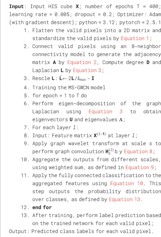
Algorithm 1. Proposed MS-GWCN for HIS classification.

3 Results

3.1 Dataset and experimental setup

We evaluated MS-GWCN on three standard hyperspectral benchmarks: Indian Pines (IP), Salinas (SA), and Pavia University (PU), which will be discussed in detail in later sections (Khoshsokhan et al., 2019a; Khoshsokhan et al., 2019b).

1. IP Dataset: The dataset was acquired using the AVIRIS sensor at the IP test site in northwestern Indiana. It covers 145 by 145 pixels and consists of 224 spectral reflectance bands, spanning a wavelength range from 0.4 to 5 × 10⁻⁶ m. In the experiment, 20 noise and water-absorbed bands were removed, resulting in 204 bands utilized. Sixteen ground-truth classes are shown in Figure 2a.

2. SA Dataset: The SA dataset was collected from the Salinas Valley in California, USA, in 1998 using the 224-band AVIRIS sensor. It covers an area of 512 by 217 pixels and demonstrates an impressive spatial resolution of 3.7 m per pixel. Like the IP dataset, it omits 20 water absorption bands and is displayed in an at-sensor radiance format. Sixteen classes are depicted in Figure 3a.

3. PU Dataset: The PU dataset was obtained using the Reflective Optical System Imaging Spectrometer (ROSIS) at PU in northern Italy in 2001. The uncorrected dataset comprises 115 spectral bands in the range of 43–86 μm. The image dimensions are 610 × 340 pixels, with a spatial resolution of 3 m. After removing twelve noise bands, 103 bands remain available for analysis. The dataset includes nine distinct land cover classes. Figure 4 illustrates the ground-truth map, categorizing the available data into nine classes.

Figure 2

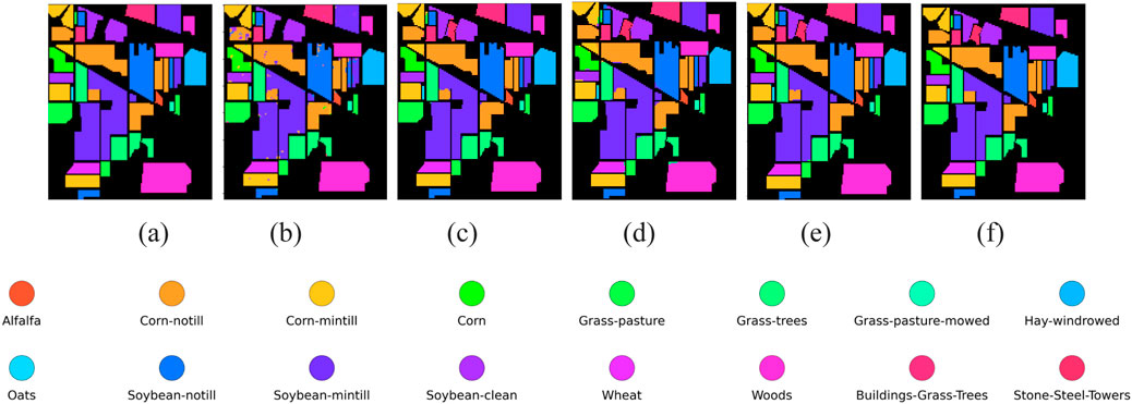
Figure 2. Classification maps on the IP dataset (a) Ground truth (b) 3D-CNN (c) MDGCN (d) AMGCFM (e) DSM-S²GCN (f) MS-GWCN.

Figure 3

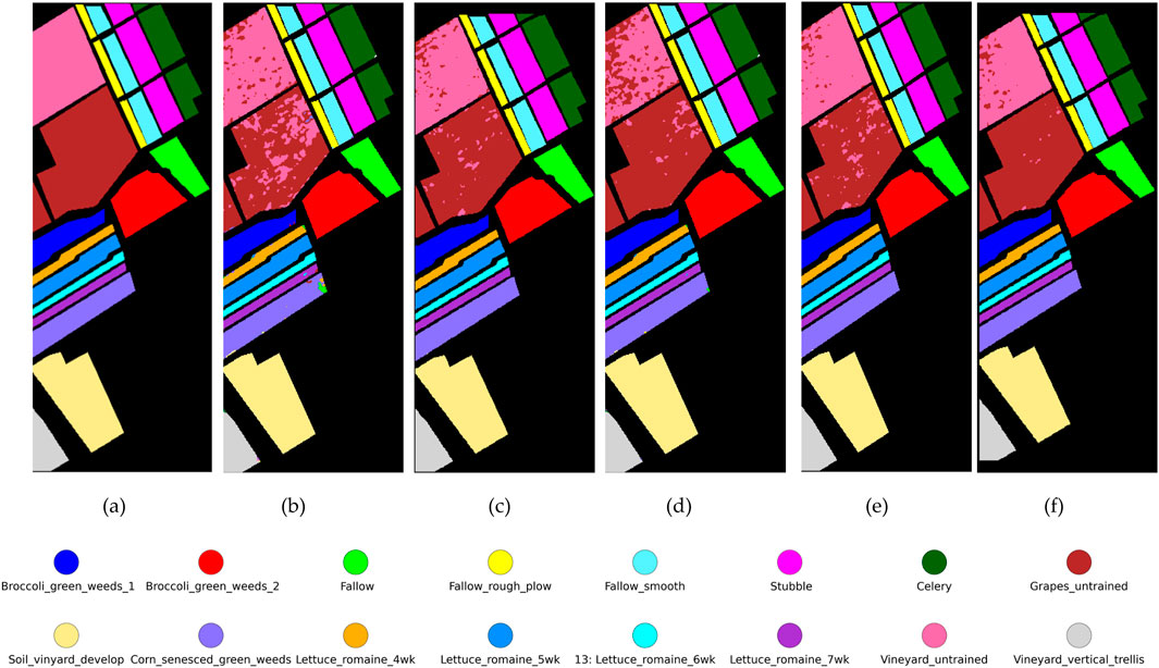
Figure 3. Classification maps on the SA dataset. (a) Ground truth (b) 3D-CNN (c) MDGCN (d) AMGCFM (e) DSM-S² GCN (f) MS-GWCN.

Figure 4

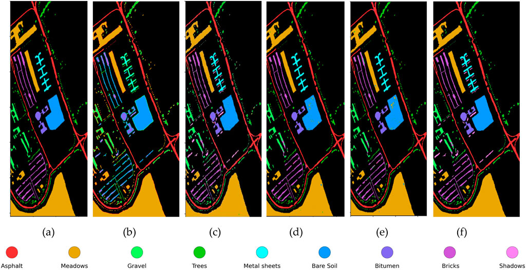
Figure 4. Classification maps on the PU dataset. (a) Ground truth (b) 3D-CNN (c) MDGCN (d) AMGCFM (e) DSM-S²GCN (f) MS-GWCN.

Table 1 summarizes the dataset sizes and train/test splits. All images were reshaped to $\left(\text{pixels}\right)\times \left(\text{bands}\right)$ vectors and normalized to zero mean and unit variance per pixel. We randomly partitioned each dataset into 80% training and 20% testing samples, ensuring all classes are represented. MS-GWCN was implemented in PyTorch (running on an NVIDIA GPU) with a unified architecture for all datasets. We trained for 400 epochs using the Adam optimizer (initial learning rate $5\times 10^{-4}$ with StepLR decay, $\gamma =0.9$ every 400 epochs), applying dropout (rate 0.5) and weight decay to reduce overfitting. All methods were run four times, and the results were averaged (mean ± std) to assess stability. Baseline methods include a 3D convolutional network (3D-CNN) (Li et al., 2017), Multi-scale Dynamic Graph Convolutional Network (MDGCN) (Wan et al., 2020), Adaptive Multi-Feature Graph Convolutional Network (AMGCFM) (Zhou et al., 2023), and a dual-stream spectral–spatial Graph Convolutional Network (DSM-S²GCN) (Liu et al., 2024), utilizing published or tuned hyperparameters.

Table 1

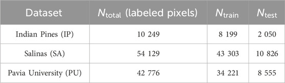
Table 1. Dataset statistics for IP, SA, and PU: total number of labeled pixels and 80:20 train-test split.

3.2 Evaluation metrics

We utilized per-class classification accuracy, overall classification accuracy (OA), average classification accuracy (AA), and the Kappa coefficient ($\kappa$) as performance evaluation metrics. OA is the fraction of correctly labeled pixels; AA is the mean of per-class accuracies; and κ measures the agreement between predicted and true labels normalized by chance (κ = 1 indicates perfect agreement). Formally, if $n_{ij}$ is the number of pixels of true class i predicted as class j, with $N={\displaystyle \sum _{i,j}}{n}_{ij}$ total pixels and C classes, then OA, AA, and $\kappa$ are represented as Equations 14–16:

$\text{OA}=\frac{1}{N_{\text{test}}}{\displaystyle \sum _{i=1}^{N_{\text{test}}}}\mathbf{1}\left({\widehat{y}}_i=y_i\right)(14)$

$\text{AA}=\frac{1}{C}{\displaystyle \sum _{c=1}^C}\frac{{\displaystyle {\sum }_{i=1}^{N_{\text{test}}}}1\left({\widehat{y}}_i=y_i=c\right)}{{\displaystyle {\sum }_{i=1}^{N_{\text{test}}}}1\left(y_i=c\right)}(15)$

$\kappa =\frac{P_0-P_e}{1-P_e},P_o=\text{OA},P_e={\displaystyle \sum _{c=1}^C}\left(\frac{{\displaystyle {\sum }_{i=1}^{N_{\text{test}}}}1\left({\widehat{y}}_i=c\right)}{N_{\text{test}}}\right)\left(\frac{{\displaystyle {\sum }_{i=1}^{N_{\text{test}}}}1\left(y_i=c\right)}{N_{\text{test}}}\right)(16)$

where $N_{\text{test}}$ is the number of test samples, C is the number of classes, ${\widehat{y}}_i$ and ${\widehat{y}}_i$ are the predicted and true labels of pixel i, 1(⋅) is the indicator function.

3.3 Comparison and analysis

As shown in Tables 2–4, the proposed method outperforms other compared frameworks on the OA, AA, and κ metrics for all three public datasets. On the IP dataset, MS-GWCN stands out as the top-performing model, achieving 100% accuracy across all classes, as well as excellent scores in OA, AA, and κ. This indicates that MS-GWCN is highly reliable and stable, with nearly flawless performance across the board. 3D-CNN follows closely, delivering strong overall performance (OA: 99.05%, AA: 98.61%, κ(×100): 98.52) with near-perfect accuracy (>99%) in agricultural and forest-related categories, such as Corn-notill (98.44% ± 0.14%), Soybean-clean (98.91% ± 0.35%), Grass-trees (99.92% ± 0.02%), and Woods (99.81% ± 0.03%). This strong performance of 3D-CNN provides reassurance to the audience about its reliability. However, its performance dips in specific classes, such as Alfalfa (95.89% ± 2.89%) and Oats (92.31% ± 5.27%), suggesting limitations in handling underrepresented or spectrally complex targets. AMGCFM achieves moderate metrics (OA: 97.99%, AA: 95.73%) but suffers significant volatility, excelling in Corn-notill (97.71% ± 5.58%) and Hay-windrowed (99.91% ± 0.36%) while collapsing in Alfalfa (89.50% ± 25.42%) and Stone-Steel-Towers (86.93% ± 23.04%). Similarly, MDGCN exhibits class-specific inconsistencies, achieving 100% accuracy in Alfalfa, Oats, and Wheat but struggling in complex classes such as Corn (76.16% ± 2.71%) and Soybean-clean (80.65% ± 7.78%), resulting in the lowest overall metrics (OA: 93.47%, κ(×100): 92.55). DSM-S²GCN is the least effective model, with an overall accuracy (OA) of 87.25%, which is significantly lower than that of the other models. Despite perfect accuracy in Grass-pasture-mowed and Oats, it fails catastrophically in critical classes like Corn (76.16% ± 2.71%) and Soybean-notill (80.65% ± 7.78%), highlighting its inability to generalize across diverse spectral features.

Table 2

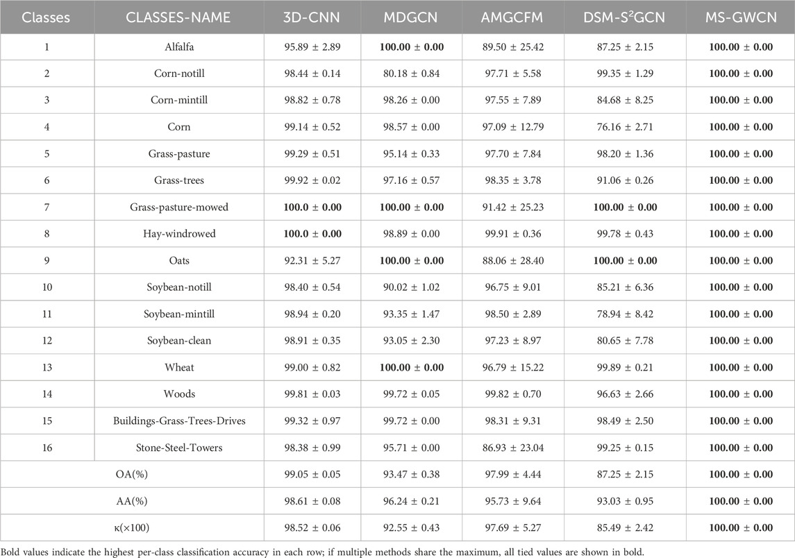
Table 2. Accuracy (%) of the different methods on the IP dataset.

Table 3

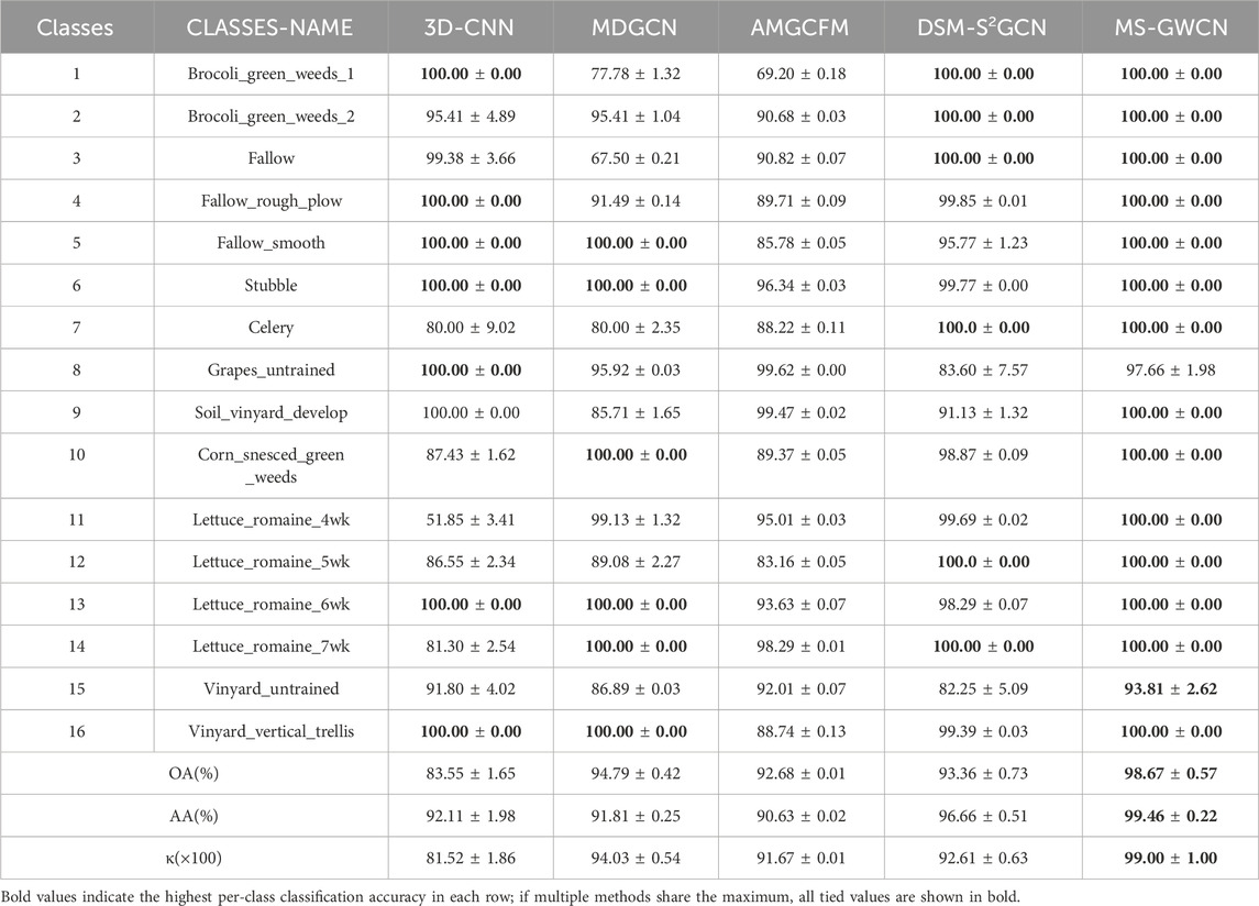
Table 3. Accuracy (%) of the different methods on the SA dataset.

Table 4

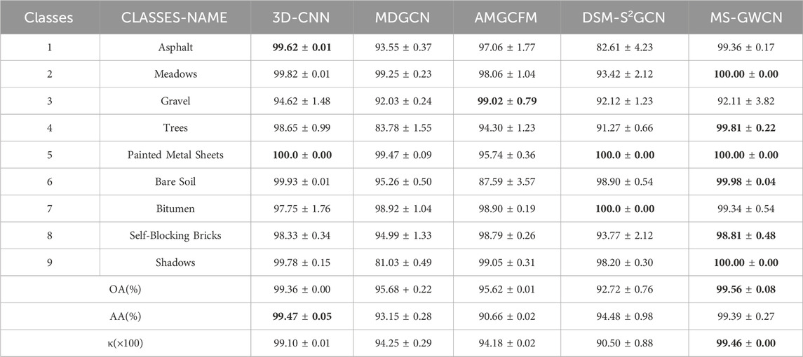
Table 4. Accuracy (%) of the different methods on the PU dataset.

Furthermore, to evaluate MS-GWCN’s generalization ability with limited training data, we conducted an experiment on the IP dataset using reduced training sample sizes. We found that even when only 50% of the original training labels were used, MS-GWCN still achieved an overall accuracy above 98% on the IP test set, only slightly lower than with the full training set. This accuracy remained significantly higher than that of the 3D-CNN baseline under the same conditions (approximately 95% OA with 50% training data). Even with only 10% of the training samples, MS-GWCN attained around 90% OA, whereas the 3D-CNN’s accuracy dropped to roughly 85%. These results demonstrate that MS-GWCN can learn effectively from very limited labeled data and still outperform conventional models, highlighting its strong generalization capability.

On the SA dataset (Table 3), MS-GWCN emerges as the unequivocal leader, achieving 100.00% ± 0.00% accuracy in 13 out of 16 classes (e.g., Broccoli_green_weeds_1, Fallow_smooth, Vinyard_vertical_trellis) and near-perfect overall metrics (OA: 98.67% ± 0.57%, AA: 99.46% ± 0.22%, κ(×100): 99.00 ± 1.00). Its zero standard deviation (±0.00) in dominant classes underscores exceptional stability, likely attributable to its advanced multi-scale graph operations for spatial-spectral feature integration. However, minor accuracy drops in Grapes_untrained (97.66% ± 1.98%) and Vinyard_untrained (93.81% ± 2.62%) suggest room for refinement in handling spectrally ambiguous or underrepresented targets. DSM-S²GCN, on the other hand, ranks second in overall accuracy (OA: 93.36% ± 0.73%) and exhibits polarized class performance. It achieves flawless results in Brocoli_green_weeds_1 (100.00% ± 0.00%) and Stubble (99.77% ± 0.00%) but struggles with Grapes_untrained (83.60% ± 7.57%) and Vinyard_untrained (82.25% ± 5.09%). Despite these limitations, its potential for future improvement is evident, offering hope for its future performance. Similarly, MDGCN (OA: 94.79% ± 0.42%) demonstrates class-specific excellence, attaining 100% accuracy in Fallow_smooth, Stubble, and Lettuce_romaine_7wk. Yet, catastrophic failures in Fallow (67.50% ± 0.21%) and Soil_vinyard_develop (85.71% ± 1.65%) reveal critical vulnerabilities in handling heterogeneous or low-sample-size categories. 3D-CNN delivers the weakest overall performance (OA: 83.55% ± 1.65%) despite sporadic successes such as 100% accuracy in Fallow_rough_plow and Vinyard_vertical_trellis. Severe underperformance in Lettuce_romaine_4wk (51.85% ± 3.41%) and Celery (80.00% ± 9.02%), coupled with high variability, underscores its instability for complex agricultural scenes. AMGCFM (OA: 92.68% ± 0.01%) exhibits erratic behavior, excelling in Lettuce_romaine_7wk (98.29% ± 0.01%) but collapsing in Brocoli_green_weeds_1 (69.20% ± 0.18%) and Fallow (90.82% ± 0.07%), with extreme standard deviations (e.g., ±0.18 in Brocoli_green_weeds_1) indicating sensitivity to training conditions.

In the PU (Table 4), MS-GWCN reaffirms its dominance, achieving 99.56% ± 0.08% OA, 99.39% ± 0.27% AA, and κ: 99.46 ± 0.00, the highest metrics among all methods. It delivers 100.00% ± 0.00% accuracy in critical classes, such as Meadows, Painted Metal Sheets, and Shadows, with near-perfect performance in Asphalt (99.36% ± 0.17%) and Bare Soil (99.98% ± 0.04%). Its minimal standard deviations (e.g., ±0.00 in Shadows) underscore exceptional stability, solidifying its superiority in spectral-spatial feature integration. 3D-CNN ranks second (OA: 99.36% ± 0.01%, AA: 99.47% ± 0.05%, κ(×100): 99.10 ± 0.01), excelling in Painted metal sheets (100.00% ± 0.00%) and Bare Soil (99.93% ± 0.01%). However, it exhibits moderate volatility in Gravel (94.62% ± 1.48%) and Bitumen (97.75% ± 1.76%), revealing sensitivity to spectrally complex surfaces. AMGCFM (OA: 95.62% ± 0.01%, AA: 90.66% ± 0.02%) demonstrates high variability, collapsing in Bare Soil (87.59% ± 3.57%) despite strong results in Gravel (99.02% ± 0.79%) and Self-Blocking Bricks (98.79% ± 0.26%). Its erratic performance (e.g., ±3.57% in Bare Soil) questions its reliability for real-world deployment and suggests caution in its use. MDGCN (OA: 95.68% ± 0.22%, κ(×100): 94.25 ± 0.29) struggles in classes requiring fine-grained discrimination, Severe underperformance in Shadows (81.03% ± 0.49%) and Trees (83.78% ± 1.55%). Moderate accuracy in Asphalt (93.55% ± 0.37%) and Self-Blocking Bricks (94.99% ± 1.33%). DSM-S²GCN ranks last (OA: 92.72% ± 0.76%, κ: 90.50 ± 0.88), with catastrophic failures in Asphalt (82.61% ± 4.23%) and Meadows (93.42% ± 2.12%). Despite achieving perfect scores in Bitumen (100.00% ± 0.00%) and Painted metal sheets (100.00% ± 0.00%), its inability to generalize across classes, such as Gravel (92.12% ± 1.23%), highlights architectural limitations.

We conduct a qualitative analysis to intuitively demonstrate the classification results and compare the classification performance of different methods. Figures 2–4 qualitatively illustrate that MS-GWCN consistently produces classification maps that are virtually identical to the ground truth, sharply delineating class boundaries and eliminating the salt-and-pepper noise and mislabeling that afflict competing methods. On IP (Figure 2), MS-GWCN achieves perfect accuracy, even in spectrally confounding regions such as Soybean-mintill, whereas 3D-CNN and MDGCN suffer from scattered misclassifications, and AMGCFM struggles along complex borders. Similarly, on SA (Figure 3), MS-GWCN’s map exhibits the cleanest and most coherent segmentation of field parcels, markedly reducing noise relative to AMGCFM and preserving delicate structures missed by 3D-CNN and MDGCN. Finally, on PU (Figure 4), MS-GWCN captures subtle building-and-road interfaces with unmatched precision and maintains structural integrity in homogeneous areas, outperforming all baselines in spatial consistency. These results demonstrate MS-GWCN’s superior capacity to model intricate spectral–spatial patterns and to generalize robustly across datasets.

To evaluate generalization with limited labels, we reduced IP training samples. With 50% of labels, MS-GWCN still achieved >98% OA (vs. ∼95% for 3D-CNN). With only 10% of labels, MS-GWCN attained ∼90% OA (vs. ∼85% for 3D-CNN). These results highlight MS-GWCN’s sample efficiency and robustness.

3.4 Influence of parameters

To elucidate the contributions of our two principal innovations,multi-scale graph wavelet convolution (MS-GWC) and explicit graph-structure representation. We conducted a focused ablation study. In Section 3.4.1, we modify the number of wavelet scales (i.e., the number of parallel GCNConv branches in each GraphWaveletConv layer) to evaluate how the scale count influences feature richness and classification. In Section 3.4.2, we examine the impact of spatial graph connectivity. The foundational MS-GWCN architecture, training hyperparameters, and data splits remain unchanged throughout each experiment.

3.4.1 Impact of different wavelet-scale counts

Our implementation of GraphWaveletConv(in_channels, out_channels, wavelet_scales = k) establishes k parallel GCNConv layers and synthesizes their outputs, effectively extracting features at k “wavelet” resolutions. To evaluate the optimal number of scales, we trained four variants of MS-GWCN on the hyperspectral dataset, setting wavelet_scales to 3, 5, 6, and 8. All other configurations were constants, including the three-layer GraphWaveletConv stack, hidden dimensions, optimizer, learning rate schedule, and 4-neighborhood graph connectivity. The line plot visualizes the performance of MS-GWCN across different wavelet scales (3, 5, 6, and 8) for the IP, SA, and PU datasets. The plot including the metrics for Overall Accuracy (OA,%), Average Accuracy (AA,%), and the Kappa coefficient (κ, ×100) are presented in Figure 5.

Figure 5

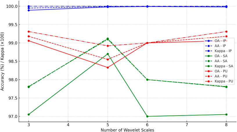
Figure 5. Performance of MS-GWCN for different Wavelet Scales.

Figure 5 shows that even with as few as three parallel wavelet channels, MS-GWCN achieves nearly 99.9% OA, demonstrating the power of graph-based spectral–spatial filtering. Moreover, increasing to five or six scales yields incremental gains, with six scales producing the highest OA (99.99%) and the smallest run-to-run variance. Furthermore, there are diminishing returns beyond six. Using eight scales does not improve upon six and incurs extra computational costs. These results indicate that six wavelet channels strike the best balance between representational richness and efficiency, and we adopt wavelet_scales = 6 for all subsequent experiments.

Meanwhile, on the IP dataset, with just three scales, MS-GWCN achieves near-saturation performance (OA: 99.90% ± 0.05%, AA: 99.80% ± 0.10%, κ(×100): 99.95 ± 0.03). Expanding to six scales maximizes accuracy (OA: 99.99% ± 0.01%, AA: 99.99% ± 0.01%, κ(×100): 99.99 ± 0.01) while minimizing run-to-run variance (±0.01). Beyond six scales, the metrics plateau (e.g., eight scales: OA = 99.90%), confirming redundancy in higher-scale spectral–spatial filtering. On the SA dataset, utilizing three wavelet scales yields a modest baseline performance with an OA of 97.05% ± 0.24%, AA of 97.81% ± 0.20%, and a κ(×100) of 97.80 ± 0.11. Expanding to five scales yields a substantial improvement, with OA increasing to 98.70% ± 0.18%, AA rising to 99.10% ± 0.14%, and Kappa reaching 99.12 ± 0.13. This increase highlights the benefit of incorporating additional spectral–spatial filtering channels in capturing the diverse vegetation classes and intricate spatial textures characteristic of Salinas. However, when increasing to six scales, the performance unexpectedly declines to OA = 97.00 ± 0.00%, AA = 98.00 ± 0.00%, and Kappa = 98.00 ± 0.00, indicating possible over-parameterization or redundancy among filters at that level. Returning to eight scales reproduces the results from the three-scale analysis (OA = 97.05 ± 0.24%, AA = 97.81 ± 0.20%, κ(×100) = 97.80 ± 0.11), confirming that beyond five scales, the model does not gain additional discriminative power while incurring extra computation. On the PU dataset, with three scales, MS-GWCN already demonstrates strong results (OA = 99.06 ± 0.04%, AA = 99.18 ± 0.12%, κ(×100) = 99.31 ± 0.07), reflecting the relatively homogeneous urban structures of this scene. Shifting to five scales slightly reduces OA to 98.33% ± 0.15% and AA to 98.55% ± 0.32%, while Kappa also dips to 98.92 ± 0.05. This decline suggests that additional scales may blur fine edges of buildings and man-made features. Increasing to six scales restores performance to a steady 99.00% ± 0.00% across OA, AA, and Kappa, indicating a more stable but not superior configuration compared to three scales. Finally, employing eight scales returns the metrics to those of the three-scale setup (OA = 99.06 ± 0.04%, AA = 99.18 ± 0.12%, κ(×100) = 99.31 ± 0.07), once again showing no net benefit beyond the three channels.

3.4.2 Impact of spatial neighborhood connectivity

To evaluate how the breadth of pixel adjacency influences MS-GWCN’s ability to exploit spatial context, we fixed the wavelet scale parameter at s = 6. We varied the graph connectivity on three benchmark datasets (IP, SA, and PU). Specifically, we compared the 2-neighborhood, where each node is connected only to its left and upper neighbors, the 4-neighborhood, which features standard cardinal connectivity (up, down, left, right), and the 8-neighborhood, which includes full connectivity with diagonals.

As depicted in Figure 6, the line plot vividly illustrates the fluctuation of OA, AA, and κ with varying spatial neighborhood connectivities (2-neighborhood, 4-neighborhood, and 8-neighborhood) for the IP, SA, and PU datasets. The progression from two to 8 neighbors amplifies MS-GWCN’s proficiency in pixel classification across all datasets (IP, SA, and PU). Notably, the IP dataset achieves a 100% OA with eight neighborhoods, indicating that more intricate pixel connectivity enables the network to comprehend spatial interdependencies, even in the most complex agricultural settings. Similarly, the SA dataset improves an OA surge from 97.19% (2-neighborhood) to 98.16% (8-neighborhood), underscoring the role of augmented spatial context in refining the classification of crops with intricate spatial textures. The PU dataset also exhibits an OA upswing from 98.97% (2-neighborhood) to 99.50% (8-neighborhood), confirming that a richer spatial relationship facilitates a more precise classification of urban land-cover categories, especially around complex borders.

Figure 6

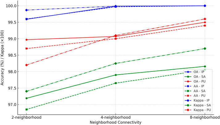
Figure 6. Performance of MS-GWCN with varing spatial neighborhood connectivity.

Meanwhile, the AA metric, which represents the average classification accuracy across all classes, also shows improvement as neighborhood connectivity becomes richer. On the IP dataset, the AA increases from 99.60% (2-neighborhood) to 100% (8-neighborhood), suggesting that the MS-GWCN can correctly classify more challenging classes (e.g., mixed-pixel regions or crops with subtle spectral differences) when pixel adjacency is expanded. On the SA dataset, the AA improves from 96.85% (2-neighborhood) to 98.05% (8-neighborhood), indicating that the expanded neighborhood enables the network to capture better complex inter-class relationships, particularly in agricultural landscapes with heterogeneous vegetation types. On the PU dataset, the AA jumps from 98.70% (2-neighborhood) to 99.40% (8-neighborhood), demonstrating that larger neighborhood contexts are beneficial in urban settings, where features such as roads, buildings, and other artificial structures require fine spatial delineation.

Moreover, the κ(×100), which quantifies the agreement between predicted and actual labels while correcting for chance, increases as the neighborhood size expands, particularly in the IP and PU datasets. On the IP dataset, the κ(×100) reaches 100 with the 8-neighborhood setting, indicating perfect agreement with the true ground labels and reflecting the MS-GWCN’s ability to handle complex spatial dependencies across the dataset. On the SA dataset, the Kappa value increases from 97.40 (2-neighborhood) to 98.70 (8-neighborhood), reinforcing the notion that richer pixel connectivity enhances the model’s spatial feature aggregation, particularly in regions with finer textures. On the PU dataset, the Kappa improves from 98.20 (2-neighborhood) to 99.60 (8-neighborhood), indicating that more neighbors enable the model to better classify fragmented urban classes, especially in areas where smaller features (e.g., roofs or pavements) require more spatial context.

Figures 7–11, collectively illustrate how MS-GWCN responds to wavelet-scale configurations and spatial-graph connectivities on three benchmarks. In Figures 7–11, we vary the number of wavelet channels on the datasets. A consistent pattern emerges, indicating that incorporating additional scales enhances smoother regional delineation and more distinct class boundaries. At low scale counts (e.g., three channels), small clusters of misclassified pixels persist around object edges; by contrast, six or eight scales produce markedly cleaner maps.

Figure 7

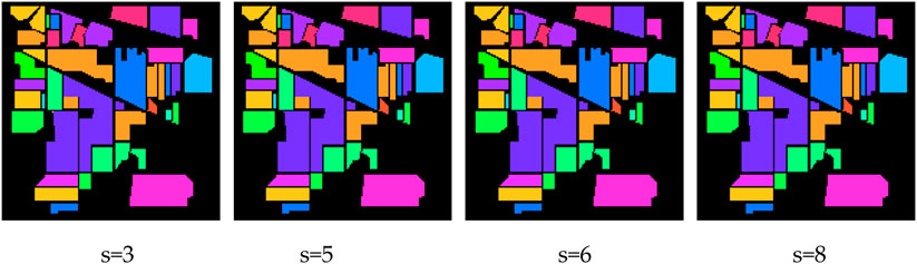
Figure 7. Classification maps achieved by different wavelet scales on the IP dataset.

Figure 8

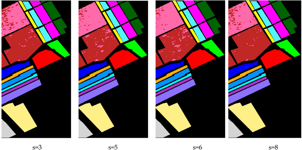
Figure 8. Classification maps achieved by different wavelet scales on the SA dataset.

Figure 9

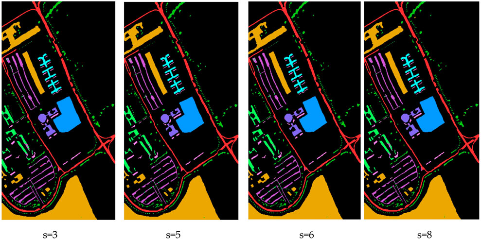
Figure 9. Classification maps achieved by different wavelet scales on the PU dataset.

Figure 10

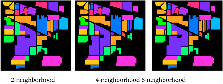
Figure 10. Classification maps achieved by different neighborhoods on the IP dataset.

Figure 11

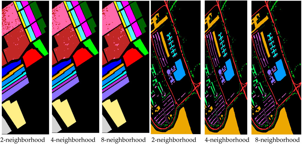
Figure 11. Classification results achieved by different neighborhoods on the SA/PU datasets.

Figures 10, 11 compare classification results using 2-, 4-, and 8-neighborhood graphs. As pixel adjacency expands, the maps become increasingly coherent. For Indian Pines (Figure 10), the 8-neighborhood graph nearly eliminates all stray errors, resulting in almost flawless segmentation. As shown in Figure 11, the Salinas also benefits, particularly in heterogeneous regions like vineyards and lettuce fields, where enhanced connectivity bridges isolated misclassifications. On Pavia University, stronger linkages unify fragmented urban classes and sharpen small-scale features such as roof tiles and pavement. Comparative results demonstrate that combining multi-scale wavelet filtering with extended spatial connections yields more accurate and stable classification maps. These qualitative observations show strong alignment with quantitative metrics, providing compelling validation of our methodology. They also confirm the effectiveness of MS-GWCN’s joint spectral-spatial fusion, supporting our final architectural choices for the model.

3.5 Computational complexity and inference time

We analyze the computational complexity of MS-GWCN and compare it with the baseline models. Thanks to the Chebyshev polynomial approximation used in the graph wavelet transform (Section 2.2), the per-layer complexity of MS-GWCN is $O\left(K\left|\mathcal{E}\right|\right)$, which is linear in the number of graph edges (with K = 3 and $\left|\mathcal{E}\right|\approx 8\left|\mathcal{V}\right|$ for an 8-neighbor graph). This is a substantial improvement over naive spectral graph convolution (which is $O\left({\left|\mathcal{V}\right|}^3\right)$) and ensures our approach can scale to reasonably large HSIs. In terms of model size, MS-GWCN contains on the order of 10⁵–10⁶ trainable parameters in our implementation, which is considerably smaller than a typical 3D-CNN-based HSI classifier (such models can require tens of millions of parameters). As a result, MS-GWCN is relatively lightweight compared to deep CNN counterparts.

In practice, we observed that the inference time of MS-GWCN is comparable to or better than that of the 3D-CNN baseline. For example, processing the entire Indian Pines image (145 × 145 pixels with 200 spectral bands) with a trained MS-GWCN takes on the order of a few seconds on a modern GPU, which is similar to the 3D-CNN’s inference time for the same data. Multi-scale graph convolutions incur overhead; however, a smaller parameter budget and an efficient Chebyshev approximation limit both memory and runtime. The resulting complexity remains tractable and is justified by the observed accuracy improvements.

4 Conclusion

This paper introduces MS-GWCN, a novel multi-scale graph wavelet convolutional network for hyperspectral image classification. The proposed framework effectively captures local and global contextual information by integrating multi-scale spectral-spatial feature extraction with graph wavelet transforms, enabling more accurate and robust classification. Our experiments on three public benchmark datasets (IP, SA, and PU) demonstrate that MS-GWCN not only outperforms existing state-of-the-art methods but does so consistently across multiple evaluation metrics, including per-class accuracy, overall accuracy (OA), average accuracy (AA), and the Kappa coefficient (κ). These results robustly demonstrate the effectiveness of our model. Large-scale hyperspectral datasets demand efficient processing. Our approach addresses this by implementing Chebyshev polynomial approximation during graph wavelet transformation, dramatically lowering computational demands. In practical implementation, satisfactory classification results are achieved with only three wavelet convolution layers and 400 training epochs, reflecting the model’s practicality and computational economy.

Despite these promising results, our MS-GWCN approach has some limitations. First, the multi-scale graph wavelet framework introduces additional computational overhead compared to simpler models. However, we mitigated this with efficient approximations, and the model’s adaptability reassures us that it can be scaled to huge images or real-time applications with further optimization. Second, the current implementation uses a fixed 8-neighborhood graph structure, which may not capture very long-range pixel relationships beyond the local vicinity; an adaptive graph construction or incorporation of global connections could further improve performance in scenes with large-scale structures. Third, performance is hyperparameter-dependent (scale count, depth, etc.), and achieving the best results typically calls for some dataset-specific tuning. Finally, MS-GWCN assumes that the training and test data come from similar distributions, its accuracy may degrade if the model is applied to data with entirely new spectral characteristics or significant noise without retraining. We acknowledge these limitations as directions for future improvements.

For future research, we plan to investigate the potential of MS-GWCN in multimodal graph learning settings and its applicability to more complex and heterogeneous remote sensing scenes. This ongoing development should leave you feeling excited about the future of our model. We anticipate that these efforts will further enhance the model’s capabilities and broaden its applicability in real-world scenarios.

Data availability statement

Publicly available datasets were analyzed in this study. This data can be found here: https://www.ehu.eus/ccwintco/index.php/Hyperspectral_Remote_Sensing_Scenes.

Author contributions

HZ: Conceptualization, Methodology, Formal Analysis, Writing – review and editing. JK: Conceptualization, Methodology, Formal Analysis, Investigation, Writing – original draft, Writing – review and editing. JZ: Methodology, Writing – review and editing.

Funding

The author(s) declare that financial support was received for the research and/or publication of this article. This work was supported by the Hainan Provincial Natural Science Foundation of China under Grant No. 621RC599.

Conflict of interest

The authors declare that the research was conducted in the absence of any commercial or financial relationships that could be construed as a potential conflict of interest.

Generative AI statement

The author(s) declare that no Generative AI was used in the creation of this manuscript.

Any alternative text (alt text) provided alongside figures in this article has been generated by Frontiers with the support of artificial intelligence and reasonable efforts have been made to ensure accuracy, including review by the authors wherever possible. If you identify any issues, please contact us.

Publisher’s note

All claims expressed in this article are solely those of the authors and do not necessarily represent those of their affiliated organizations, or those of the publisher, the editors and the reviewers. Any product that may be evaluated in this article, or claim that may be made by its manufacturer, is not guaranteed or endorsed by the publisher.

References

Anderson, J., and Cheng, J. (2023). Spectral graph wavelet transform for multiscale hyperspectral image classification. IEEE Trans. Geoscience Remote Sens. 56 (12), 7315–7325. doi:10.1016/j.patrec.2023.01.003

CrossRef Full Text | Google Scholar

Behmanesh, M., Adibi, P., Ehsani, M. S., and Chanussot, J. (2024). “Geometric multimodal deep learning with multi-scaled graph wavelet convolutional network,” in IEEE Transactions on Neural Networks and Learning Systems. 35 (5), 6991–7005. doi:10.48550/arXiv.2111.13361

CrossRef Full Text | Google Scholar

Cai, W., Jiang, J., and Qian, J. (2023). Large-scale hyperspectral image restoration via a superpixel distributed algorithm based on graph signal processing. IEEE Trans. Geoscience Remote Sens. 61, 1–17. doi:10.1109/TGRS.2023.3242728

CrossRef Full Text | Google Scholar

Cao, B., and Messinger, D. W. (2025). Spatial-spectral graph convolutional network for automatic pigment mapping of historical artifacts. npj Herit. Sci. 13, 106. doi:10.1038/s40494-025-01629-7

CrossRef Full Text | Google Scholar

Ding, Y., Feng, J., Chong, Y., Pan, S., and Sun, X. (2022). Adaptive sampling toward a dynamic graph convolutional network for hyperspectral image classification. IEEE Trans. Geoscience Remote Sens. 60, 1–17. doi:10.1109/TGRS.2021.3132013

CrossRef Full Text | Google Scholar

Ding, Y., Zhang, Z., Hu, H., He, F., Cheng, S., and Zhang, Y. (2024). Graph neural network for feature extraction and classification of hyperspectral remote sensing images. Singapore: Springer Verlag.

Google Scholar

Dong, Y., Liu, Q., Du, B., and Zhang, L. (2022). Weighted feature fusion of convolutional neural network and graph attention network for hyperspectral image classification. IEEE Trans. Image Process. 31, 1559–1572. doi:10.1109/TIP.2022.3144017

PubMed Abstract | CrossRef Full Text | Google Scholar

Hammond, D. K., Vandergheynst, P., and Gribonval, R. (2011). Wavelets on graphs via spectral graph theory. Appl. Comput. Harmon. Analysis 30 (2), 129–150. doi:10.1016/j.acha.2010.04.005

CrossRef Full Text | Google Scholar

He, X., Chen, Y., and Ghamisi, P. (2022a). Dual graph convolutional network for hyperspectral image classification with limited training samples. IEEE Trans. Geoscience Remote Sens. 60, 1–18. doi:10.1109/TGRS.2021.3061088

CrossRef Full Text | Google Scholar

He, M., Wei, Z., and Wen, J. R. (2022b). Convolutional neural networks on graphs with chebyshev approximation, revisited. Adv. neural Inf. Process. Syst. 35, 7264–7276. doi:10.48550/arXiv.2202.03580

CrossRef Full Text | Google Scholar

Hughes, G. (1968). On the mean accuracy of statistical pattern recognizers. IEEE Trans. Inf. Theory 14 (1), 55–63. doi:10.1109/TIT.1968.1054102

CrossRef Full Text | Google Scholar

Kang, X., Li, S., and Benediktsson, J. A. (2014). Spectral–spatial hyperspectral image classification with edge-preserving filtering. IEEE Trans. Geoscience Remote Sens. 52 (5), 2666–2677. doi:10.1109/TGRS.2013.2264508

CrossRef Full Text | Google Scholar

Khoshsokhan, S., Rajabi, R., and Zayyani, H. (2019a). Clustered multitask non-negative matrix factorization for spectral unmixing of hyperspectral data. J. Appl. Remote Sens. 13 (2), 1–026509. doi:10.1117/1.jrs.13.026509

CrossRef Full Text | Google Scholar

Khoshsokhan, S., Rajabi, R., and Zayyani, H. (2019b). Sparsity-constrained distributed unmixing of hyperspectral data. IEEE J. Sel. Top. Appl. Earth Observations Remote Sens. 12 (4), 1279–1288. doi:10.1109/jstars.2019.2901122

CrossRef Full Text | Google Scholar

Kipf, T. N., and Welling, M. (2016). Semi-supervised classification with graph convolutional networks. arXiv Prepr. arXiv:1609.02907. doi:10.48550/arXiv.1609.02907

CrossRef Full Text | Google Scholar

Li, Y., Zhang, H., and Shen, Q. (2017). Spectral–spatial classification of hyperspectral imagery with 3D convolutional neural network. Remote Sens. 9, 67. doi:10.3390/rs9010067

CrossRef Full Text | Google Scholar

Liu, Q., Zhou, F., Hang, R., and Yuan, X. (2017). Bidirectional-convolutional LSTM based spectral-spatial feature learning for hyperspectral image classification. Remote Sens. 9, 1330. doi:10.3390/rs9121330

CrossRef Full Text | Google Scholar

Liu, Q., Xiao, L., Yang, J., and Wei, Z. (2021). CNN-enhanced graph convolutional network with pixel and superpixel level feature fusion for hyperspectral image classification. IEEE Trans. Geoscience Remote Sens. 59 (10), 8657–8671. doi:10.1109/TGRS.2020.3037361

CrossRef Full Text | Google Scholar

Liu, S., Li, H., Jiang, C., and Feng, J. (2024). Spectral–spatial graph convolutional network with dynamic-synchronized multiscale features for few-shot hyperspectral image classification. Remote Sens. 16, 895. doi:10.3390/rs16050895

CrossRef Full Text | Google Scholar

Ma, W., Gong, C., Hu, Y., Meng, P., and Xu, F. (2000). “The Hughes phenomenon in hyperspectral classification based on the ground spectrum of grasslands in the region around Qinghai Lake,” Proc. SPIE 8910, International Symposium on Photoelectronic Detection and Imaging 2013: Imaging Spectrometer Technologies and Applications. 89101G. doi:10.1117/12.2034457

CrossRef Full Text | Google Scholar

Melgani, F., and Bruzzone, L. (2004). Classification of hyperspectral remote sensing images with support vector machines. IEEE Trans. Geoscience Remote Sens. 42 (8), 1778–1790. doi:10.1109/TGRS.2004.831865

CrossRef Full Text | Google Scholar

Pu, S., Wu, Y., Sun, X., and Sun, X. (2021). Hyperspectral image classification with localized graph convolutional filtering. Remote Sens. 13, 526. doi:10.3390/rs13030526

CrossRef Full Text | Google Scholar

Shen, Y., Dai, W., Li, C., Zou, J., and Xiong, H. (2021). Multi-scale graph convolutional network with spectral graph wavelet frame. IEEE Trans. Signal Inf. Process. over Netw. 7, 595–610. doi:10.1109/TSIPN.2021.3109820

CrossRef Full Text | Google Scholar

Uddin, M. P., Mamun, M. A., and Hossain, M. A. (2020). PCA-Based feature reduction for hyperspectral remote sensing image classifica-Tion. IETE Tech. Rev. 38 (5), 377–396. doi:10.1080/02564602.2020.1740615

CrossRef Full Text | Google Scholar

Vasudevan, V., Bassenne, M., Islam, M. T., and Xing, L. (2017). Image classification using graph neural network and multiscale wavelet superpixels. Pattern Recognit. Lett. 166, 89–96. doi:10.1016/j.patrec.2023.01.003

CrossRef Full Text | Google Scholar

Wan, S., Gong, C., Zhong, P., Du, B., Zhang, L., and Yang, J. (2020). Multiscale dynamic graph convolutional network for hyperspectral image classification. IEEE Trans. Geoscience Remote Sens. 58 (5), 3162–3177. doi:10.1109/TGRS.2019.2949180

CrossRef Full Text | Google Scholar

Yang, J. Y., Li, H. C., Hu, W. S., Pan, L., and Du, Q. (2022a). Adaptive cross-attention-driven spatial-spectral graph convolutional network for hyperspectral image classification. IEEE Geosci. Remote Sens. Lett. 19, 1–5. doi:10.1109/LGRS.2021.3131615

CrossRef Full Text | Google Scholar

Yang, B., Cao, F., and Ye, H. (2022b). A novel method for hyperspectral image classification: deep network with adaptive graph structure integration. IEEE Trans. Geoscience Remote Sens. 60, 1–12. doi:10.1109/TGRS.2022.3150349

CrossRef Full Text | Google Scholar

Yu, W., Wan, S., Li, G., Yang, J., and Gong, C. (2023). Hyperspectral image classification with contrastive graph convolutional network. IEEE Trans. Geoscience Remote Sens. 61, 1–15. doi:10.1109/TGRS.2023.3240721

CrossRef Full Text | Google Scholar

Zhang, C., and Ma, Y. (2012). Ensemble machine learning: methods and applications. doi:10.1007/9781441993267

CrossRef Full Text | Google Scholar

Zhang, Y., Duan, P., Mao, J., Kang, X., Fang, L., and Ghamisi, P. (2022). Contour structural profiles: an edge-aware feature extractor for hyperspectral image classification. IEEE Trans. Geoscience Remote Sens. 60 (1–14), 1–14. doi:10.1109/tgrs.2022.3229075

CrossRef Full Text | Google Scholar

Zhang, Y., Duan, P., Liang, L., Kang, X., Li, J., and Plaza, A. (2025a). PFS3F: probabilistic fusion of superpixel-wise and semantic-aware structural features for hyperspectral image classification. IEEE Trans. Circuits Syst. Video Technol., 1. doi:10.1109/TCSVT.2025.3556548

CrossRef Full Text | Google Scholar

Zhang, Y., Liang, L., Mao, J., Wang, Y., and Jia, L. (2025b). From global to local: a dual-branch structural feature extraction method for hyperspectral image classification. IEEE J. Sel. Top. Appl. Earth Observations Remote Sens. 18, 1778–1791. doi:10.1109/JSTARS.2024.3509538

CrossRef Full Text | Google Scholar

Zhou, H., Luo, F., Zhuang, H., Weng, Z., Gong, X., and Lin, Z. (2023). Attention multihop graph and multiscale convolutional fusion network for hyperspectral image classification. IEEE Trans. Geoscience Remote Sens. 61, 1–14. doi:10.1109/TGRS.2023.3265879

CrossRef Full Text | Google Scholar