EPIC and NISTAR radiometric stability assessment using ERA5 reanalysis data

A technique to determine the radiometric stability of the Earth Polychromatic Imaging Camera (EPIC) and the National Institute of Standards and Technology Advanced Radiometer (NISTAR), the two Earth-viewing instruments operating aboard the Deep Space Climate Observatory (DSCOVR) satellite, which is orbiting the Sun at the Lagrange-1 point, L₁, approximately 1.5 million kilometers away from Earth, has been developed and applied. Apart from the satellite’s own measurements, it only uses output from the European Centre for Medium-Range Weather Forecasts (ECMWF) atmospheric reanalysis of the global climate data center (ERA5). This method can be applied to all channels (and not just a subset) and can be repeated periodically to track the instruments’ stability. The method includes the removal of climatological diurnal and seasonal cycles, a multivariate regression fitting with selected ERA5 model output parameters, and referencing the data to the EPIC 551-nm channel, which has been determined to show no drift over the entire mission lifetime together with the NISTAR photodiode channel (200–1,100 nm). The obtained sensitivity changes were very small, ranging from a maximum total degradation of 3% over 10 years in the short UV (<340 nm) to no detectable changes for some channels. For the EPIC UV channels, the derived results were confirmed through a comparison of the EPIC data with radiances from the Ozone Mapping and Profiler Suite (OMPS). We attribute this excellent instrument performance mostly to the L₁ orbit, which is not only an ideal location for Earth observation, but is also extremely beneficial (quiet) with respect to instrument performance. At L_1, there are only minor temperature variations and much smaller exposure to charged particles from the Sun compared to satellites orbiting the Earth, which are fully or partly inside the Earth’s radiation belts. In this sense, L₁ can be considered “observational and instrumental heaven.” The technique described here could only be applied because DSCOVR has two different instruments (EPIC and NISTAR) observing the same Earth flux input. This suggests that it is extremely useful (maybe even essential) to combine imaging instruments (like EPIC) with integrating instruments (like NISTAR) in remote sensing applications.

1 Introduction

The Earth Polychromatic Imaging Camera (EPIC) and the National Institute of Standards and Technology Advanced Radiometer (NISTAR) are the two Earth-viewing instruments operating aboard the Deep Space Climate Observatory (DSCOVR) satellite, which is orbiting the Sun at the Lagrange-1 point, L₁, approximately 1.5 million kilometers away from the Earth (Marshak et al., 2018). Both instruments measure the solar radiance backscattered from the sunlit portion of the Earth. EPIC provides spatial images for 10 narrowband wavelength filters, from the ultraviolet (UV) to the near-infrared (NIR) region (Cede et al., 2021), and its data products include total column ozone and sulfur dioxide, aerosol, cloud, ocean surface and vegetation properties, reflectivity, and atmospheric correction (Marshak et al., 2018). NISTAR measures the integrated signal over the entire Earth’s disk in four broadband channels (NASA GSFC, 2025) and is primarily used to determine the total daytime Earth radiative flux and changes in the planetary albedo (Su et al., 2020; Lacis et al., 2022). The quality of the higher-level data products from both instruments directly depends on the retrieved radiances in each channel and therefore is sensitive to potential instrumental drifts over time. For this reason, the calibration stabilities of EPIC and NISTAR have been analyzed by various groups using different methods in the past:

• Wen and Marshak (2023) used Moderate-Resolution Imaging Spectroradiometer (MODIS) data and EPIC lunar observations for the oxygen A- and B-bands absorbing channels 7 (688 nm) and 9 (764 nm). From the comparison to the MODIS, the authors state that “one can see that there is no noticeable trend in the data and the observed differences are within the range of variation of the ratios.”

• Su et al. (2018) used MODIS and Earth’s Radiant Energy System (CERES) broadband measurements for channels 5 (442 nm), 6 (551 nm), and 8 (680 nm) and found no drift compared to CERES in the year 2017.

• Doelling et al. (2019a) used MODIS and Suomi National Polar-Orbiting Partnership Visible Infrared Imaging Radiometer Suite (NPP-VIIRS) data for channels 5 (442 nm), 6 (551 nm), 8 (680 nm), and 10 (779 nm). They state that “the EPIC four-year calibration trends based on VIIRS are within 0.15%/year.”

• Geogdzhaev et al. (2021) used data from MODIS, NPP-VIIRS, and the Multi-angle Imaging Spectroradiometer (MISR) for channels 5 (442 nm), 6 (551 nm), 8 (680 nm), and 10 (779 nm). The derived calibration trends in this study were all below 0.3% per year with only the trend of channel 5 being significant.

• Haney et al. (2021) used MODIS, VIIRS, and Invariant Targets on ground for all non-UV channels, i.e., channels 5 (442 nm), 6 (551 nm), 7 (688 nm), 8 (680 nm), 9 (764 nm), and 10 (779 nm). The study concludes that “EPIC bands 5 and 6 degraded mostly within the first year of operation and became stable thereafter, whereas bands 7 and 10 were stable during the 6-years record.” The record analyzed was from 2015 to 2021, and the mentioned degradation of channels 5 and 6 during 2015 was at the order of 2%.

• Su et al. (2021) used the technique from their paper published in 2018 to derive broadband shortwave radiances from EPIC channels 5 (442 nm), 6 (551 nm), and 8 (680 nm). They state “Furthermore, annual global daytime mean SW fluxes from EPIC agree with the CERES equivalents to within 0.5 Wm⁻² with root-mean-square errors less than 3.0 Wm⁻².” Since the SW flux is around 200 W m⁻², this corresponds to ∼0.25%.

In most cases, the papers listed above mention the very good and stable radiometric performance of EPIC. EPIC has even been used to radiometrically validate other satellite instruments (Doelling et al., 2019b). All methods applied in these studies rely on comparisons of the EPIC data with low Earth orbit (LEO) satellites or observations of special targets on the Moon or Earth. As such, a substantial effort in establishing these comparisons goes into adjusting for different viewing geometries, finding appropriate collocations, data filtering procedures, angular corrections, etc.

In this paper, we present a different method for deriving the radiometric stability of all 10 EPIC channels and two of the NISTAR channels. The concept of this technique is to build a time series of the data and correct them as best as possible for input variations (i.e., real variations of the backscattered signal from Earth) so that only the instrumental changes remain. The following is the basic procedure:

1. The EPIC and NISTAR data are corrected for those influencing parameters for which the exact correction factors are known, namely, the varying Earth-DSCOVR distance (EDD) and Earth–Sun distance (ESD).

2. A climatological diurnal and annual cycle for all channels is formed from nearly 10 years of data and used to deseasonalize the time series.

3. A multivariate linear regression in a similar way as used for other long term data records (Herman et al., 2023 or Borger et al., 2022) is applied. The influencing parameters used are the Sun–Earth-DSCOVR (or Sun–Earth-Vehicle) angle (SEV-angle), and data from the fifth-generation ECMWF atmospheric reanalysis of the global climate (ERA5) (Hersbach et al., 2023).

4. After the previous corrections, the remaining time series is analyzed for similarities between EPIC and NISTAR. Since those are two entirely different instruments, all correlated data variations can be attributed to residual effects of the Earth flux, which were not captured in the steps before.

5. The remnant is smoothed and is considered an estimation of the sensitivity change of the instruments over time.

One big advantage of the method described in this paper is that it can be applied to all EPIC channels, not just a subset, and can be repeated periodically to track the instruments’ stability.

This paper shows the basics of this method and the application for all 10 EPIC channels and 2 NISTAR channels to the DSCOVR time series from the “first light” (June 2015) to the end of 2024. In addition, the obtained results were validated through a separate method, where the four EPIC UV channels were compared to data from the Suomi National Polar-orbiting Partnership OMPS Nadir Mapper (OMPS-NM) (Flynn et al., 2014). The results were also compared to the statements about the instrument stability from the existing literature.

2 Materials and methods

2.1 DSCOVR orbital data

The DSCOVR orbital data are shown in Figure 1. They were obtained in hourly intervals from the Jet Propulsion Laboratory (JPL) Horizons System (NASA JPL, 2025). The ESD varies by ±1.67% around 1 astronomical unit (1 AU = 1.49598 × 10⁸ km). The EDD varies from −7.70% to +6.92% around the chosen L₁ reference of 1.5 × 10⁶ km, and the SEV-angle ranges from 1.83° on 2 June 2021° to 12.36° on 14 October 2021. Both the ESD and EDD change the total signal in the instruments by their squares. The combined effect of ESD and EDD on the total signal received by the instrument is shown as a dashed black line in the bottom panel and ranges from −17.26% on 23 January 2024 to +18.12% on 14 July 2018 relative to the reference position at 1 AU and 1 L₁. The varying EDD also causes a change in the “size of the Earth” on the EPIC detector. Figure 2 shows as an example the EPIC RGB images for the largest and smallest EDD in the time series.

Figure 1

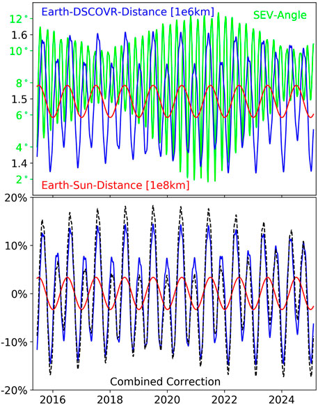
Figure 1. Top: Earth–Sun-Distance (ESD, red in units of 10⁸ km), Earth-DSCOVR distance (EDD, blue in units of 10⁶ km) and Sun–Earth-Vehicle angle (SEV-angle, green, in degrees) as a function of time. The green label refers to the SEV-angle, and the black label to ESD and EDD. Bottom: data correction in percent relative to the reference at 1 AU and 1 L₁ due to ESD only (red), EDD only (blue) and the combined effect of ESD and EDD (dashed black) as a function of time.

Figure 2

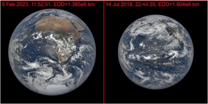
Figure 2. EPIC RGB images at the moment of the smallest EDD on 5 February 2023 (left panel) and the largest EDD on 14 July 2018 (right panel) in the DSCOVR time series (images from the EPIC website https://epic.gsfc.nasa.gov/). The SEV-angle is 6° in both cases. All time indications in this paper are UTC.

2.2 EPIC data

EPIC has 10 narrowband filters from 317 nm to 780 nm (Table 1). We will refer to them as “EPIC 317 nm”, “EPIC 325 nm”, etc., where the given wavelength is the (rounded) wavelength center of the respective filter. The exact wavelengths, resolutions (ranging from 0.9 to 3.0 nm Full-Width at Half Maximum) and invariant exposure times (ranging from 22 to 654 ms) can be found in Cede et al. (2021).

Table 1

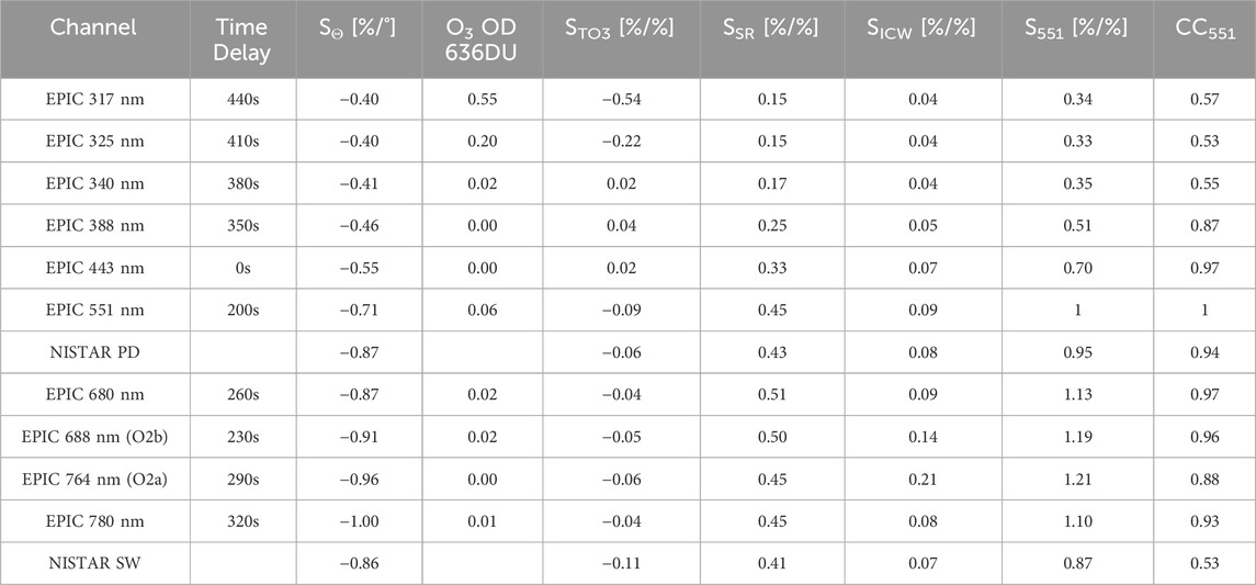
Table 1. Specifications and results for the EPIC and NISTAR channels. “Time Delay” is the typical time difference of the measurement of an EPIC channel relative to EPIC 443 nm. S_Θ is the sensitivity of the signal to the SEV-angle in % per degree. O₃ OD 636DU is the ozone optical depth for 636DU (the only reason we chose 636DU here is because this happens to be the value for which the OD best matches the values of S_TO3, as shown in Section 4.2). S_TO3, S_SR, and S_ICW are the sensitivities to TO3, SR, and ICW, respectively. S₅₅₁ and CC₅₅₁ are the sensitivity and correlation coefficient of the signal in a channel to the signal in EPIC 551 nm, respectively.

The EPIC level 1A (L1A) data used for this analysis are from the latest production version v03 and can be obtained from NASA EOSDIS (2025). The signal in each pixel is proportional to the radiance as it is already corrected for a list of instrumental effects such as dark count, latency, detector non-linearity, temperature, flat field, and stray light (Cede et al., 2021). Conversion factors from counts/second to radiance are given in Marshak et al. (2018), and updates can be found on the web under https://epic.gsfc.nasa.gov/science/calibration/uv, https://epic.gsfc.nasa.gov/science/calibration/visnir, and https://epic.gsfc.nasa.gov/science/calibration/o2channels for the UV, Vis/NIR, and O2-absorbing channels, respectively. The data used here are the sum over all pixels of the L1A images in each channel, given in resolution of 2048 × 2048, which corresponds to the irradiance (or flux) from Earth reaching EPIC. This quantity also depends on the EDD, which affects the object size on the detector and thus requires correction (Figure 2).

There are a total of 47,877 full EPIC sequences (i.e., where all 10 channels were measured) until the end of 2024. A nominal measurement sequence starts with channel EPIC 443 nm, ends with EPIC 317 nm, and lasts approximately 7 min and 20 s. This means that at the equator, the Earth has rotated approximately 200 km during the measurement sequence. The typical time delay of a channel relative to the EPIC 443 nm channel is given in Table 1. Note that the rows in the table are sorted by wavelength and not in the order the EPIC channels were measured.

From the 47,877, we have filtered out 3,542 image sequences due to different reasons such as incomplete metadata, unusual measurements duration (>8 min or <5.5 min), non-operational image read mode, non-nominal exposure times, bad pointing (where the image of the Earth is clipped), or lunar influence (the Moon covering part of the Earth’s image or transiting behind the Earth). This leaves a total of 44,335 image sequences. A time series of the residuals of the flux measured by EPIC is shown in Figure 3. Here, residual means the percentage difference relative to the mean value over the entire time series. These data have only been corrected for the varying ESD and EDD.

Figure 3

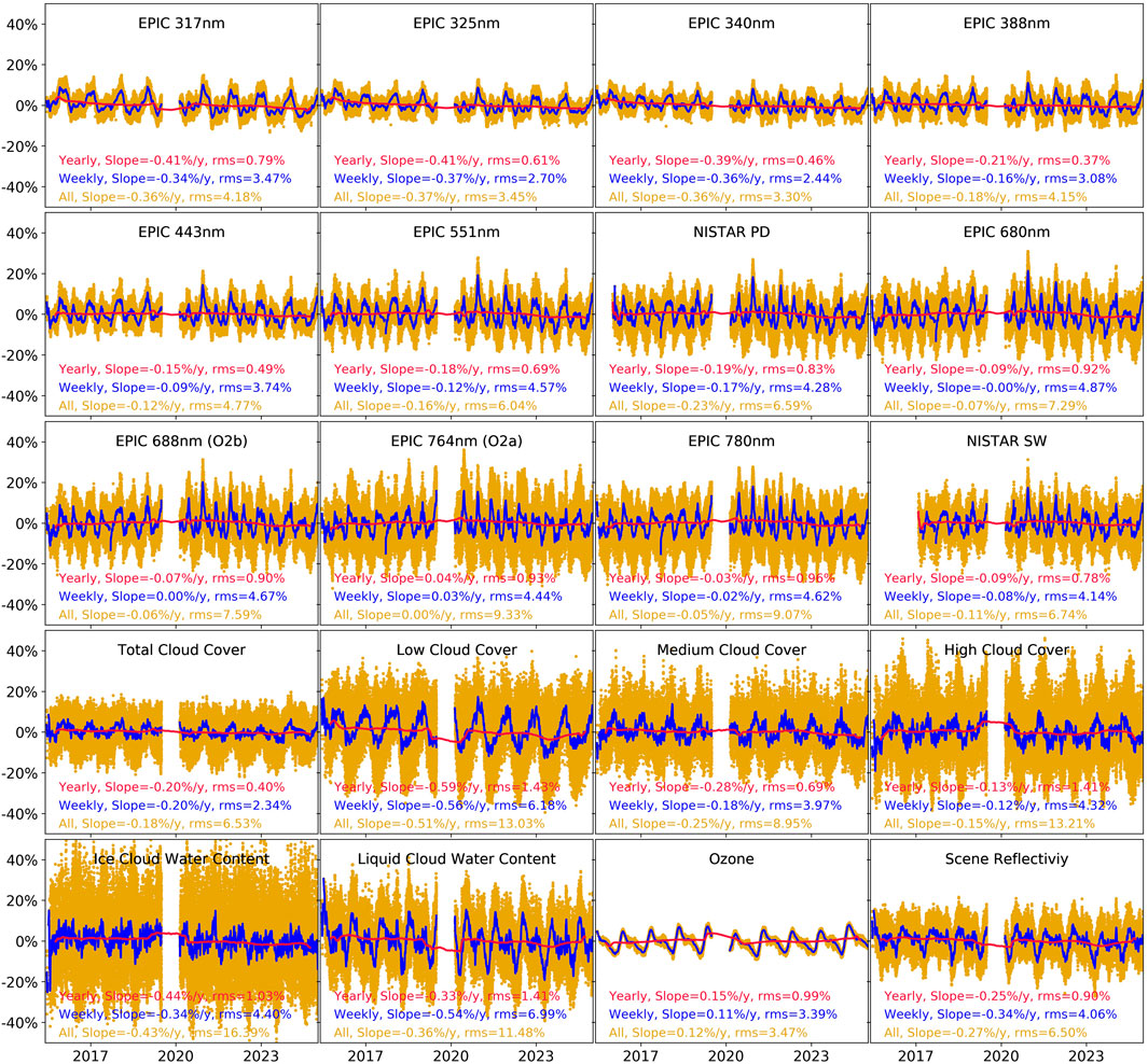
Figure 3. Time series of the residuals of the total flux measured by EPIC and NISTAR (top three rows) and of the ERA5 model outputs (bottom two rows, which will be explained in Section 3.4). Residuals are the percentage difference to the mean value over the entire time series. The x-labels mark the beginning of the respective year. All (44,335) data are shown in gold, running weekly averages in blue and running yearly averages in red. The legend at the bottom of each panel shows results from a linear fit in time of the data and gives the slope in percent per year and the rms in percent.

The period from 16 June 2015 to 31 December 2024 spans over 3,487 days, of which EPIC has taken measurements on 3,088 days. Most of the missing days are due to a DSCOVR safe hold period, which lasted from 27 June 2019 to 19 February 2020, totaling nearly 9 months (note the gap in the data in Figure 3 around the beginning of the year 2020). Reasons for the safe hold were issues with DSCOVR’s attitude control system (NOAA NESDIS, 2020). There are also a number of missing measurement days at the beginning of the mission, where different spacecraft and instrument tests were performed. The first day, where at least 10 EPIC observations were done, was 3 August 2015. Finally, some days do not have measurements since the Moon was observed instead of the Earth for calibration purposes (Geogdzhaev et al., 2021).

Out of the 44,335 filtered EPIC sequences, we made daily means and also running weekly and yearly means, i.e., averages of the data spanning 7 or 365 days, centered around each measurement day. The (running) weekly and yearly averages are also shown in Figure 3. Note that the yearly mean during the safehold period is obviously impaired by the missing data since it covers effectively only 3 months.

When doing a simple linear regression in time on this data, we can see that most EPIC channels give a slightly negative drift over time reaching up to −0.4% per year for the 317 nm channel, and the slopes do not significantly depend on the averaging width (all data versus weekly or yearly). The root mean squares (rms) of the regressions range from 3.3% to 9.3% for all data, 2.4%–4.9% for weekly means, and 0.4%–1% for yearly means.

2.3 NISTAR data

NISTAR has four broadband channels (NASA LaRC ASDC, 2016), of which two are analyzed: the photodiode, covering a wavelength range from 200 to 1,100 nm, and Band B, measuring the total solar reflected flux between 200 and 4,000 nm. Here, we call them “NISTAR PD” and “NISTAR SW,” respectively, and they are inserted in Table 1 in the approximate “effective wavelength,” which is on average somewhere between 500 and 700 nm for NISTAR PD, and probably above 1,000 nm for NISTAR SW.

The NISTAR data used for this analysis are the L1B data from the latest production version 3 and can be obtained from NASA EOSDIS (NASA LaRC ASDC, 2025). For the photodiode current, the L1B data represent a 1-s average of the original 10-Hz measurements taken during Earth observations. These data are corrected by subtracting the “dark” photocurrent measured during observations of dark space. Similarly, the shortwave radiance L1B data are derived from demodulated radiometer power, corrected using the offset determined during dark space observations, and further adjusted by a receiver-specific calibration constant and the solid angle subtended by Earth, as seen from DSCOVR (NASA LaRC ASDC, 2023).

The original NISTAR data were then averaged into 1-minute-long intervals. NISTAR PD data are given in nA (nano amperes), with the first valid data starting on 4 January 2016, and NISTAR SW is given in W/m²/sr, with the first valid data starting on 1 February 2017. Hence, the valid NISTAR time series starts somewhat later than for EPIC.

We built the mean of the 1-min data over the duration of each EPIC sequence (approximately 7 min) and corrected them for the distances ESD and EDD. Hence, the NISTAR data analyzed here correspond exactly to the times of the EPIC data, just the number of valid data is 38,245 (NISTAR PD) and 33,920 (NISTAR SW) instead of 44,335 due to the later start. In the same way as for EPIC, daily, weekly, and yearly running means were built (Figure 3). Just as for the EPIC data, both NISTAR channels show a slightly negative slope over time. Also note that the slope and rms of the NISTAR PD channel are nearly identical to EPIC 551 nm, which is an indication that the “effective” wavelength for NISTAR PD is around this region.

2.4 ERA5 data

ERA5 hourly global reanalysis data were obtained from the Copernicus Climate Store website (Hersbach et al., 2023). The ERA5 outputs used for this study were hourly global reanalysis data from 1940 to present (Copernicus Climate Change Service C3S, 2017), which have been accessed in April and May 2025. We downloaded the following parameters (names as given in ERA5): UV–visible albedo for direct radiation (A_SURF), Total cloud cover (TCC), Low cloud cover (LCC), Medium cloud cover (MCC), High cloud cover (HCC), Total column cloud ice water (ICW), Total column cloud liquid water (LCW), and Total column ozone (TO3).

In addition, we have also built a “composite” model parameter, which we call “Scene Reflectivity” (SR). SR is a combination of the albedo and cloud outputs (Equations 1, 2):

$\text{SR}=\text{TCC\hspace{0.17em}}*{\text{AC}}_{\text{EFF}}+\left(1-\text{TCC}\right)*{\mathrm{A}}_{\text{SURF}}(1)$

AC_EFF is the “effective cloud albedo”:

${\text{AC}}_{\text{EFF}}=\left(\text{LCC\hspace{0.17em}}*{\text{AC}}_{\text{LOW}}+\text{MCC\hspace{0.17em}}*{\text{AC}}_{\text{MED}}+\text{HCC\hspace{0.17em}}*{\text{AC}}_{\text{HIGH}}\right)/\left(\text{LCC}+\text{MCC}+\text{HCC}\right)(2)$

AC_LOW, AC_MED, and AC_HIGH are the cloud albedos associated with LCC, MCC, and HCC, respectively. We assume a relation of AC (=AC_LOW, AC_MED, or AC_HIGH) to the Cloud Optical Depth (COD), as given by Stephens (1978):

$\text{AC}=\text{COD}/\left(\text{COD}+\mathrm{k}\right)(3)$

For the adjustment factor k in Equation 3, we use a value of 8, as suggested by Slingo (1989). The COD is related to the cloud water content (CW, in kg/m²) in this way as given in Equation 4 (Liou, 2002):

$\text{COD}=1.5{\mathrm{m}}^3/\text{kg}/\mathrm{r}*\text{\hspace{0.17em}CW}(4)$

r is the effective cloud droplet radius, for which we assume a value of 30 µm for ice clouds and 12 µm for liquid clouds, respectively, as suggested by Han et al. (1994). For CW, we take the outputs ICW and LCW from the ERA5 reanalysis, which gives these results for the respective CODs (Equation 5):

${\text{COD}}_{\text{HIGH}}=1.5{\mathrm{m}}^3/\text{kg\hspace{0.17em}}/{\mathrm{r}}_{\text{ICE}}*\text{\hspace{0.17em}IWC}(5)$

${\text{COD}}_{\text{MED}}=1.5{\mathrm{m}}^3/\text{kg}/{\mathrm{r}}_{\text{LIQU}}*\text{\hspace{0.17em}LWC\hspace{0.17em}}*\text{\hspace{0.17em}MCC}/\left(\text{LCC}+\text{MCC}\right)$

${\text{COD}}_{\text{LOW}}=1.5{\mathrm{m}}^3/\text{kg}/{\mathrm{r}}_{\text{LIQU}}*\text{\hspace{0.17em}LWC\hspace{0.17em}}*\text{\hspace{0.17em}LCC}/\left(\text{LCC}+\text{MCC}\right)$

The native ERA5 global data outputs and the SR were down-gridded by a factor of 7 in latitude and 9 in longitude from their original grid size (0.25°) to 1.75° in latitude and 2.25° in longitude. This was done to save disk space and processing time. Then, for each DSCOVR measurement, the model data from the same time as the DSCOVR measurements covering the sunlit portion of the Earth were averaged. The sunlit portion was determined using the geolocation information from the EPIC L1A images (Blank et al., 2021). The obtained model data, except the surface albedo A_SURF, are also shown in Figure 3. A_SURF is a climatology and repeats every year in the same way and therefore has no long-term change. As for the measurements, the model residuals show the percentage deviation around their overall mean value, which was 6.8% for A_SURF, 62% for TCC, 35% for LCC and HCC, 24% for MCC, 0.0079 mm for ICW, 0.0206 mm for LCW, 290 DU for TO3, and 27% for SR.

It should be noticed that all cloud-related model outputs give a negative slope over time in the regression (see legends in the bottom of Figure 3). Such a decrease in cloudiness is also mentioned in the literature (Andersen et al., 2022; Loeb et al., 2021). The TO3 yields a slightly positive slope of approximately 1.5% per decade, which agrees with numbers about the ozone recovery from the Scientific Assessment of Ozone Depletion 2022 (WMO, 2022). Both a decrease in cloudiness and an increase in TO3 result in a decrease in the radiance measured by DSCOVR, which suggests that parts of the negative trends seen in the observations are due to a changing Earth flux.

As mentioned in the Introduction, cloud properties and TO3 are also EPIC data products, and obviously it would have been much easier to use those data for this study. However, we did not want to make statements about the instrument’s stability using its own derived data and therefore used the ERA5 data instead.

3 Results

3.1 Diurnal and seasonal cycle

In order to isolate underlying instrumental trends from regular seasonal variations, we first deseasonalize the data, which is a common practice for long data records (Chehade et al., 2014; Coldewey-Egbers et al., 2022). For this, a climatological diurnal and annual cycle for all channels was built from the nearly 10 years of data. First, all the data for a given day of the year falling into a 3-h time window centered around UTC time points of 0:00, 0:20, 0:40, etc. until 23:40 (72 bins) were averaged. Then, a smoothing spline fit with a width of 60 days and polynomial order 2 was applied to the data in each bin as a function of the day of the year. The exact same procedure has been applied to the model data from ERA5.

Figures 4, 5 show the obtained seasonal and diurnal cycles. It can be seen that, with the exception of TO3, all measured and modeled data show a very pronounced seasonal and diurnal variation. TO3 changes with the season, but on average, it does not change over the day as it is dominated by stratospheric processes. Changes in TO3 observed during the day are mostly driven by weather events with changes in pressure and are statistically random. The cycles are dominated by diurnal and seasonal cloud distribution and can be compared with results from Delgado-Bonal et al. (2020), Delgado-Bonal et al. (2021), and Delgado-Bonal et al. (2024).

Figure 4

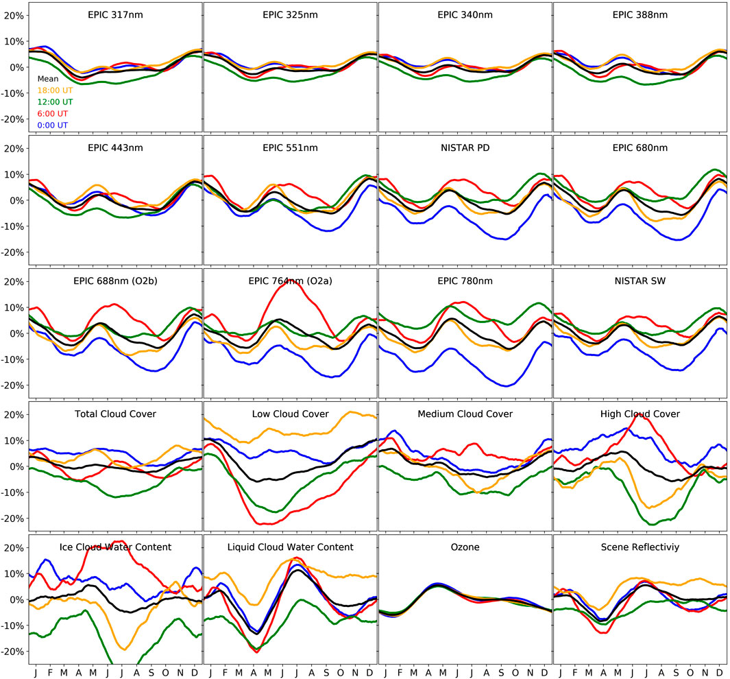
Figure 4. Seasonal cycles of the measurements (top three rows) and model outputs (bottom two rows) based on the 10-year time series. The x-labels are centered in the middle of each month. The black lines are the daily mean value, and the colored lines refer to different times of the day: blue is for 0:00, red for 6:00, green for 12:00, and yellow for 18:00 UTC.

Figure 5

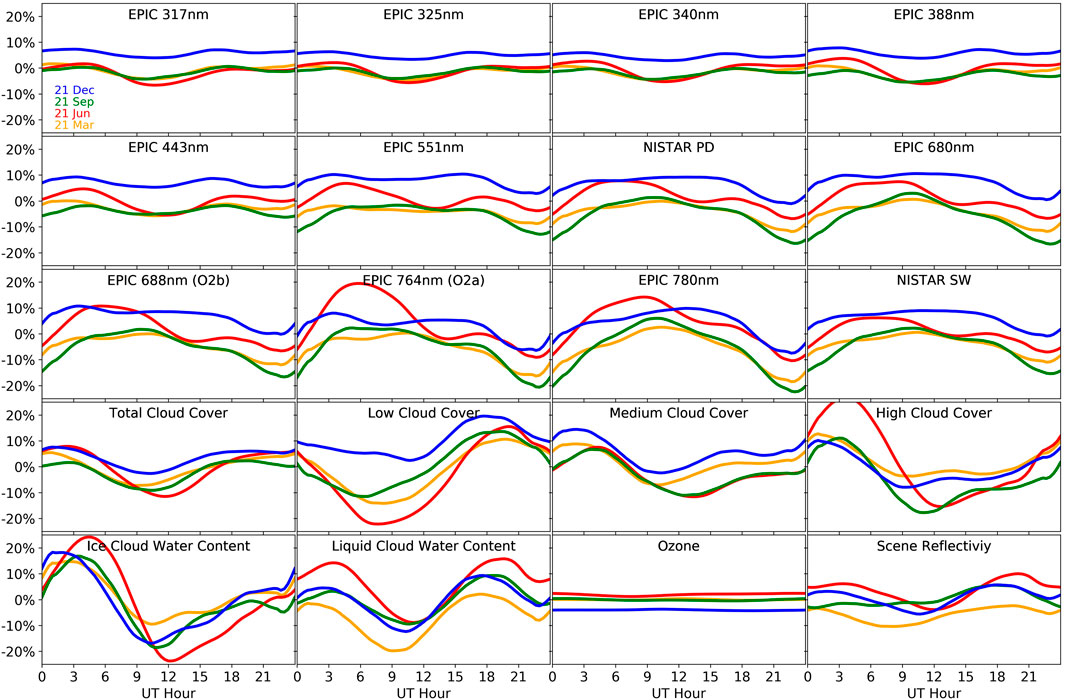
Figure 5. Diurnal cycles of the measurements (top three rows) and model outputs (bottom two rows). The different colors refer to different days of the year: yellow for 21 March, red for 21 June, green for 21 September, and blue for 21 December.

The strongest backscattered signal happens on average in December, where Antarctica is on the sunlit side of the Earth. However, in the NIR channels, the highest values are reached in June around 6:00. Figure 6 shows the mean signal for selected hours in the month of June (hence, the images in Figure 6 are associated with the red lines in Figure 5). It is made from EPIC L1B data (taken from NASA EOSDIS (2025)), which have been averaged over the entire time period for each month and hour. Note that before averaging, they have been resized to the reference EDD = 1 L₁ so that the size of their images on the detector are the same. Basically, images with smaller EDD (like the left panel in Figure 2) have been reduced, and those with larger EDD (like the right panel in Figure 2) have been increased. Figure 6 also demonstrates the capability of producing climatologies from EPIC data as its time series has already approached 10 years!

Figure 6

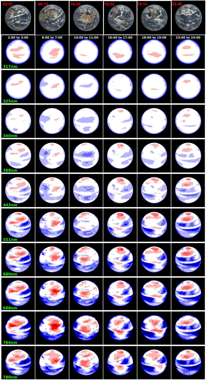
Figure 6. The first row shows EPIC RGB images from 15 June 2024, taken from the EPIC webpage. The exact time of the image is given in the top left corner. The chosen times represent situations in which different continents “face the sun” (from left to right): Australia, Asia, Africa, South America, North America, and none (just Pacific Ocean). The subsequent 10 rows show the normalized average signal for each EPIC channel in the month of June for different hours. The color scale ranges from 0.30 (dark blue) over 1 (white) to 3.3 (dark red). The panels can be compared to the red lines in Figure 5.

Figure 6 shows that the strong backscattered signal around 6:00 in June is caused by large cloud formation over Asia, which is primarily associated with the onset of the South Asian summer monsoon (Wu and Chen, 2021; Rajagopalan et al., 2017).

The time series of measurements and model data after the seasonal and diurnal correction is shown in Figure 7. While the slopes in time expectedly have not changed compared to Figure 3, the rms has been reduced by more than a factor of 2, which allows us to see other patterns in the data. In particular, one can notice the correlation of the measurements with the SEV-angle (compare the blue lines in Figure 6 with the green line in Figure 1).

Figure 7

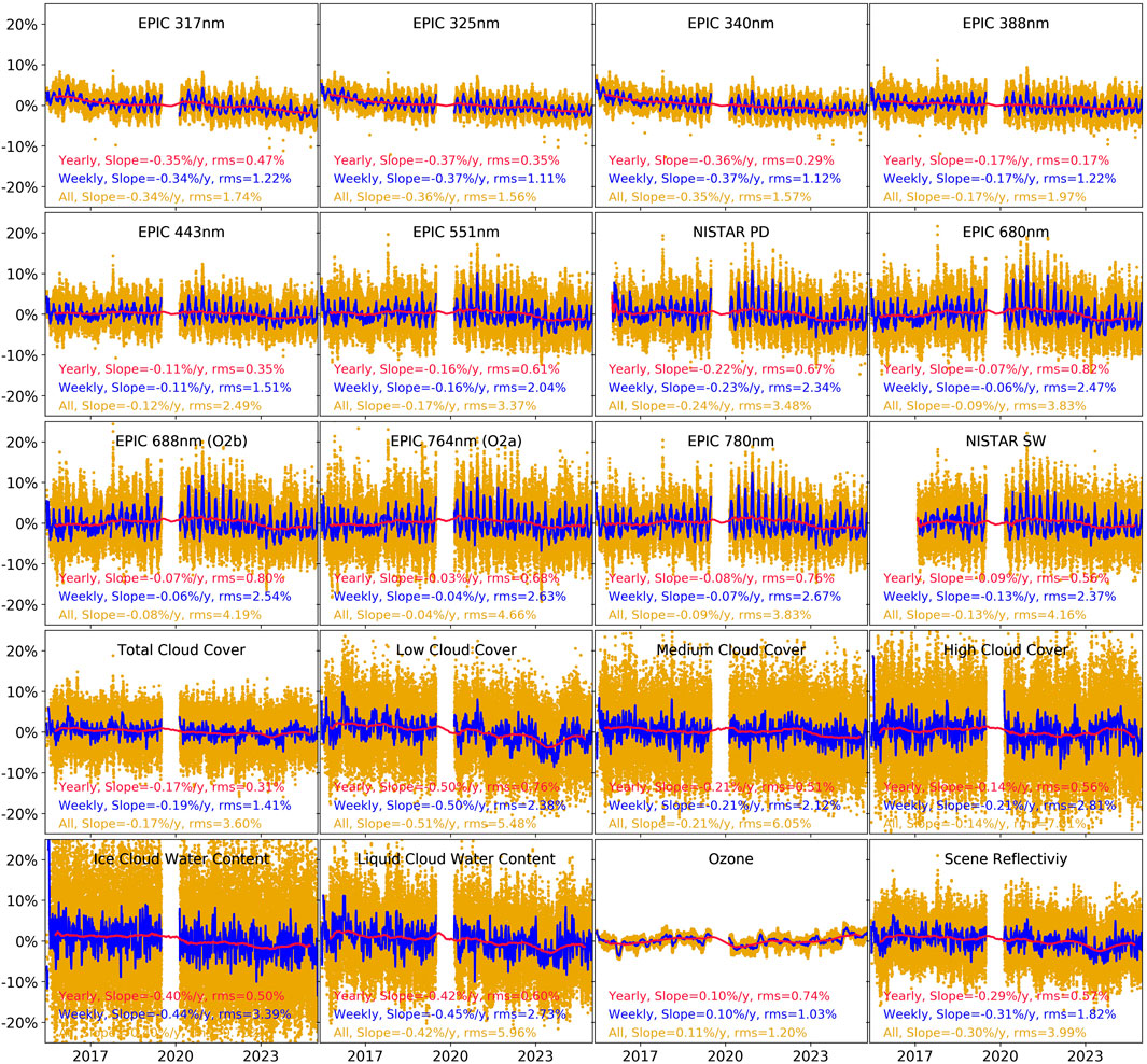
Figure 7. Time series as in Figure 3, but the data are corrected for the seasonal cycles shown in Figures 4, 5.

3.2 Multivariate linear regression

3.2.1 General fitting equation

While the relationship between the signal and the distances ESD and EDD is well known, this is not the case for the other influencing factors. To determine the sensitivity of the measurements to the different model parameters and the SEV-angle, a multivariate linear regression was applied, in a similar way as has been done in trend analysis studies (Herman et al., 2023).

The multivariate fitting follows the following equation:

${\mathrm{R}}_{\mathrm{i}}\left(\mathrm{t}\right)={\mathrm{S}}_{\text{ti}0}+{\mathrm{S}}_{\text{ti}1}·\mathrm{t}+{\mathrm{S}}_{\text{ti}2}·{\mathrm{t}}^2+\dots +{\mathrm{S}}_{\text{tiNt}}·{\mathrm{t}}^{\text{Nt}}+\leftarrow \text{\hspace{0.17em}Time\hspace{0.17em}dependence}(6)$

${\mathrm{S}}_{\mathrm{\Theta }\mathrm{i}1}·\mathrm{\Theta }\left(\mathrm{t}\right)+{\mathrm{S}}_{\mathrm{\Theta }\mathrm{i}2}·{\mathrm{\Theta }\left(\mathrm{t}\right)}^2+\dots +{\mathrm{S}}_{\mathrm{\Theta }\text{iN}\mathrm{\Theta }}·{\mathrm{\Theta }\left(\mathrm{t}\right)}^{\mathrm{N}\mathrm{\Theta }}+\leftarrow \text{\hspace{0.17em}SEV}-\text{angle\hspace{0.17em}dependence}$

${\mathrm{S}}_{\mathrm{M}1\mathrm{i}1}·\mathrm{M}1\left(\mathrm{t}\right)+{\mathrm{S}}_{\mathrm{M}1\mathrm{i}2}·{\mathrm{M}1\left(\mathrm{t}\right)}^2+\dots +{\mathrm{S}}_{\mathrm{M}1\text{iN}1}·{\mathrm{M}1\left(\mathrm{t}\right)}^{N1}+\leftarrow \text{\hspace{0.17em}Model\hspace{0.17em}output\hspace{0.17em}}1$

$\dots$

${\text{SM}}_{\text{mi}1}·\text{\hspace{0.17em}Mm}\left(\mathrm{t}\right)+{\text{SM}}_{\text{mi}2}·{\text{MM}\left(\mathrm{t}\right)}^2+\dots +{\text{SM}}_{\text{MmiN}1}·\text{\hspace{0.17em}Mm}{\left(\mathrm{t}\right)}^{\text{Nm\hspace{1em}}}\leftarrow \text{\hspace{0.17em}Model\hspace{0.17em}output\hspace{0.17em}}\mathrm{m}$

where t is the time and i is the channel index. R_i(t) is the variation (or residual) of the signal for channel i, as given in Figure 7. The “S” are the different “sensitivity coefficients” for various parameters. S_tij is the time coefficient of order j for filter i, where j can range from j = 0 to j = Nt. Θ(t) is the SEV-angle variation relative to 8° and the S_Θij are the SEV-angle sensitivity coefficients (j = 1 to NΘ). Mk(t) is the variation of model output parameter k (k = 1 to m), as given in Figure 7 with the corresponding S_Mkij, the sensitivity coefficients of order j (j = 1 to Nk). As can be seen, we have not restricted ourselves to a purely linear relationship between the measurements and any of the parameters going into the regression.

3.2.2 Choice of polynomial orders

We have tested a wide variation of options (which model parameters to use, what orders for the sensitivity coefficients of each term, etc.), and the main conclusions are as follows:

• Using a higher-order dependence for the different model data did not yield a significant improvement over the linear dependence. I.e., the reduction of the “fitting-rms” (the rms of the difference between the measurements and the fitted data) was only marginal when adding a quadratic term, and the magnitude of this term was also insignificant. This does not necessarily mean that the flux depends only linearly on cloudiness, ozone, etc. It simply means that by taking out the seasonality (Section 4.1), we have already removed much of the influence from those parameters, and for the residual effect, a linear approach is sufficient.

• When adding a quadratic dependence on the SEV-angle, we have seen a small improvement in the fitting results, i.e., a reduction in the fitting-rms. Having a small curvature is also predicted by the analytical formula for the scattering function introduced by Song et al. (2018) with an idealized spherical system illuminated by a parallel beam. However, we decided to use a linear dependence for the final selection since adding a quadratic term did not change the overall results, but we noticed some minor cross-correlation to SR, which we wanted to avoid.

• The only part of Equation 6 where we used a higher-order dependence was the time evolution. This was included to avoid the fitting of instrumental changes into the system. Nevertheless, we observed that more than a quadratic dependence in time was not necessary, i.e., higher-order terms did not significantly reduce the fitting-rms.

• While using many (or all) of the model parameters given in Figure 7 somewhat improved the fitting-rms, we also noticed that it made the system more unstable. This is because all the cloud parameters are correlated to each other since obviously the TCC is related to the LCC, MCC, and HCC and all the other cloud parameters as well. Hence, the effect of fitting several of the cloud parameters was that the results were not consistent among the different channels anymore as the model “distributed” the sensitivity coefficients nearly randomly over the model data.

• Therefore, we limited the number of cloud-related parameters used in the fitting to two. The highest correlation between the measurements and the different model parameters was given for the Scene Reflectivity (SR) since SR was “composed” specifically for that purpose. Therefore, we chose SR as the main cloud parameter.

• The other cloud parameter in addition to SR, which best improved the fitting-rms, was the Ice Cloud Water Content (ICW). ICW made an impact on the oxygen absorbing channels, which was not well-captured by the SR. Therefore, we chose ICW as the secondary cloud parameter.

• The only model parameter not correlated to any other one is the TO3. It was added in the fitting and improved the results for the short UV channels.

3.2.3 Reduced fitting equation

As a consequence of these findings, we reduced the regression model into this final version:

${\mathrm{R}}_{\mathrm{i}}\left(\mathrm{t}\right)={\mathrm{S}}_{\text{ti}0}+{\mathrm{S}}_{\text{ti}1}·\mathrm{t}+{\mathrm{S}}_{\text{ti}2}·{\mathrm{t}}^2+{\mathrm{S}}_{\mathrm{\Theta }\mathrm{i}}·\mathrm{\Theta }\left(\mathrm{t}\right)+{\mathrm{S}}_{\text{SRi}}·\text{\hspace{0.17em}SR}\left(\mathrm{t}\right)+{\mathrm{S}}_{\text{ICWi}}·\text{\hspace{0.17em}ICW}\left(\mathrm{t}\right)+{\mathrm{S}}_{\text{TO}3\mathrm{i}}·\text{\hspace{0.17em}TO}3\left(\mathrm{t}\right)(7)$

Here, we are using a quadratic dependence on time and linear dependencies in the SEV-angle, SR, ICW, and TO3. The obtained sensitivity coefficients S_Θi, S_SRi, S_ICWi, and S_TO3i from Equation 7 are shown in Figure 8 and also in Table 1. Their regression uncertainties are all very small (below 0.01).

Figure 8

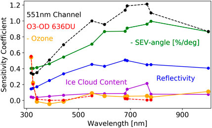
Figure 8. Sensitivity coefficients from the regression model for the SEV-angle (green), TO3 (orange), SR (blue), and ICW (purple) as a function of the “effective” wavelength for each channel (for NISTAR PD a nominal value of 600 nm was used and for NISTAR SW 1000 nm). For the SEV-angle, the unit of the coefficient is in % per °, and for all other parameters, it is in % per %. For the SEV-angle and TO3, the values are multiplied by −1, i.e., the original values are mostly negative. The red line gives the ozone optical depth (O3-OD) for a quantity of 636DU, which happens to overlap best with the negative values of the TO3 sensitivity coefficients. The black line gives the sensitivity of the measurement residuals relative to the data from the EPIC 551-nm channel. All values are also listed in Table 1.

3.2.4 Obtained sensitivities

The SEV-angle sensitivity (S_Θ in Table 1) peaks at −1% per degree for the EPIC 780-nm channel. Marshak et al. (2021) also reported the largest SEV-angle effect in the Red and NIR channels, when they studied extreme SEV-variation events of 10° difference. They even reported signal enhancements of more than 20% for a 10° reduction in the SEV-angle. We believe the values given here yield good estimates for the average SEV-angle effect on the flux in each channel.

The SR sensitivity (S_SR in Table 1) peaks at 0.5 in the red channels, which means that 1% higher SR gives half a percent increase in the flux. The ICW sensitivity (S_ICW in Table 1) is mostly important for the oxygen-absorbing channels and reached a maximum of 0.2 for EPIC 764 nm. As expected, the highest sensitivity to TO3 (S_TO3 in Table 1) is for EPIC 317 nm with −0.5 (Figure 8 shows the negative values, i.e., the values multiplied by −1). A 1% increase in TO3 reduces the signal at 317 nm for 0.5%. For ozone, the spectral dependence of the sensitivity should follow the ozone cross-sections (or optical depth). It happens to be that the ozone optical depth (O3-OD) for 636 DU (red line in Figure 8) is similar to the (negative values of the) obtained TO3 sensitivity, which is confirmation that the established procedure worked well.

3.2.5 Multivariate fitting results

The time series of the measurements, after applying the results from the regressions, are shown in Figure 9. Compared to Figure 7, the rms has again dropped significantly, but more importantly, the retrieved slopes have changed by +0.1 to +0.2%. While basically all the slopes were originally negative, now there are positive and negative ones, since based on the regression results, we know that the backscattered radiance from the Earth has slightly diminished in the past 10 years due to reduced cloudiness and the ongoing recovery of the ozone layer.

Figure 9

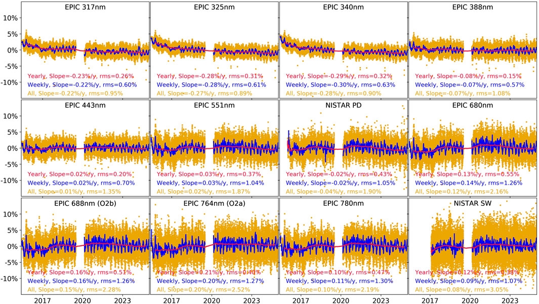
Figure 9. Time series as in Figure 7 but limited to the measurements only, and the data are also corrected by the result from the regression model.

Still, from Figure 9, one can observe residual systematic signals in the time series, which are very correlated among the different channels. Hence, there are variations in the data, which have not been explained by the corrections included so far.

3.3 EPIC 551 nm versus NISTAR PD

All the previous results (e.g., the obtained slopes in Figure 9 or sensitivities in Figure 8) suggest the EPIC 551 nm and NISTAR PD behave very similarly in many aspects. Figure 10 gives a closer look at the data from those two channels. They are highly correlated, and their ratio shows very small variation over time. Since EPIC and NISTAR are entirely different instruments, this means that most of the remaining structure seen in Figure 9 is due to a variation in the Earth flux. The only part we can possibly attribute to any sensitivity change in EPIC 551 nm or NISTAR PD is the ratio between them (blue line in bottom panel). We do not know whether this ratio is caused by (residual) flux variation affecting EPIC 551 nm and NISTAR PD in a different way, or instrumental changes of either EPIC 551 nm or NISTAR PD, or (most likely) all of these reasons. Therefore, we claim at this point that both channels show no drift in their signal within a maximum uncertainty of 0.4% (dashed red lines in the bottom panel).

Figure 10

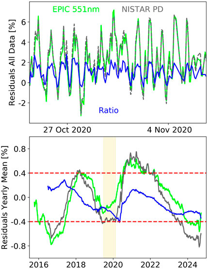
Figure 10. EPIC 551 nm (green) and NISTAR PD (gray) data (corrected for all previous steps) for a period of 2 weeks from 24 October to 7 November 2024 (top panel) and running yearly means for the entire time series (bottom panel). The ratio NISTAR PD over EPIC 551 nm is given in blue. The red dashed lines in the bottom panel show a range of ±0.4% around the zero line. The yellow area marks the DSCOVR safe hold period, during which no measurements were taken.

It turns out that the residual variation of EPIC 551 nm is not only highly correlated to NISTAR PD but also to all other channels. This is seen in the correlation coefficients (CC₅₅₁ in table 1), which range from approximately 0.55 for EPIC 317 nm, 325 nm, 340 nm, and NISTAR SW to approximately or above 0.9 for all other channels. The running yearly means from Figure 9 observed on top of each other, which is shown in the top panel of Figure 11, show the similarity in the “waves.” Again, if these were all data from the same instrument, one could not claim that this is caused by input variations, but since the EPIC and NISTAR channels are highly correlated to each other, this argument prevails.

Figure 11

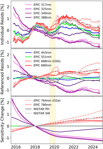
Figure 11. Top panel: Running yearly mean residuals for all channels as from Figure 9. Middle panel: Data from the top panel corrected for the signal of EPIC 551 nm. Bottom panel: Data from the middle panel smoothed. These lines can be considered to represent the change in the radiometric sensitivity for each channel over time. The yellow area marks the DSCOVR safe hold period, during which no measurements were taken.

Therefore, we decided to fit the EPIC 551 nm residual signal into the data from all other channels. The only reason we chose EPIC 551 nm over NISTAR PD is that its data series starts in 2015, which allows us to analyze a portion of that year as well. The sensitivity of the data in each channel to the residual EPIC 551-nm signal is given as a black line in Figure 8 and is also listed in Table 1. It has a regression uncertainty below 0.01 and a similar wavelength dependence as the SR- and SEV-sensitivities. It peaks at 1.2 for the EPIC 764 nm channel, which means that a signal variation caused by the flux in EPIC 551 nm of 1% causes a signal variation of 1.2% in EPIC 764 nm.

The time series of the measurements after applying this latest correction are shown in Figure 12. Compared to Figure 9, the rms has again dropped significantly, and only exceeds 1% for EPIC 764 nm and NISTAR SW. In fact, the NISTAR SW data benefit “least” from this correction, implying significantly different effects influencing this channel, which we have not further explored in this study. The slopes have not changed relative to the version from Figure 9.

Figure 12

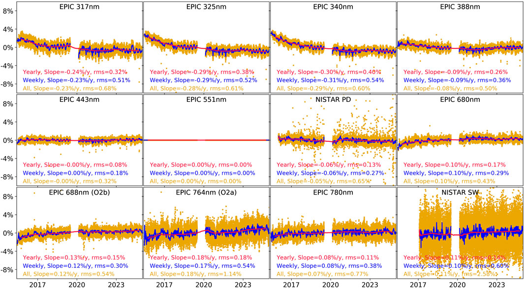
Figure 12. Time series as in Figure 9, but the data are also corrected by the signal variation in the EPIC 551-nm channel. Therefore, the panel for EPIC 551 nm is a nominal zero-line.

The new running yearly means are also displayed in the middle panel of Figure 11. Since instrumental changes do in general happen over a longer time scale, we have applied a smoothing (running polynomial of order 3 or less) to the yearly means and normalized these lines to 1 on 1 January 2018. This is shown in the bottom panel of Figure 11 and can be considered the best estimations of the sensitivity changes for each channel based on the method applied here. The same data from the bottom two panels of Figure 11 are also shown in Figure 13.

Figure 13

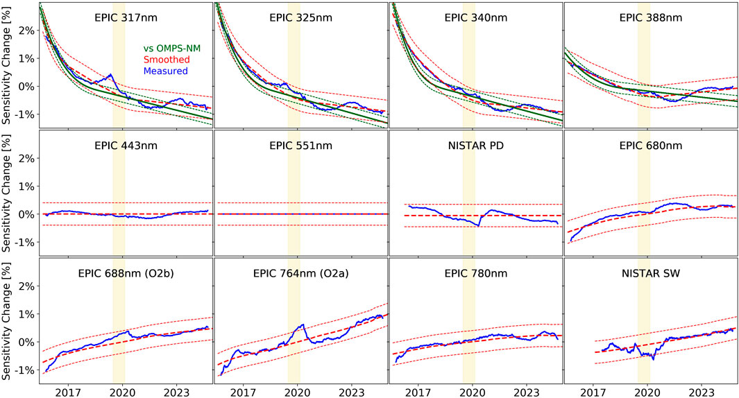
Figure 13. Time series of the running yearly means from Figure 12 (blue), the sensitivity changes derived by the regression method with uncertainty ranges (red) and the sensitivity changes for the UV channels derived from a comparison with OMPS-NM with uncertainty ranges (green). The nearly 9-month-long DSCOVR safe hold period (yellow area), during which no measurements were taken, affects the running yearly means (blue lines) in and near this time period, but should not have too large of an impact for the sensitivity changes (red lines).

The short UV channels EPIC 317 nm, 325 nm, and 340 nm show a small degradation of approximately 1% per year from the start of the mission until about the beginning of 2018, which has then flattened out to a slope below −0.2% per year since then. EPIC 388 nm was also degrading at the beginning, but by only half the amount compared to the other UV channels. We claim that no sensitivity change can be detected for EPIC 443 nm, EPIC 551 nm, and NISTAR PD. The red and NIR EPIC channels and NISTAR SW show a slightly positive trend of approximately 0.1%–0.15% per year. Overall, we can confirm the remarkable radiometric stability of both EPIC and NISTAR mentioned in the literature given in Section 1.

3.4 Validation of the method for the EPIC UV channels

OMPS-NM was launched in 2012 into a sun synchronous polar orbit and has been making Earth radiance UV spectral measurements from 298 nm to 381 nm since then. It has a global coverage in 1 day, with 14 orbits, and a spatial resolution of 50 km × 50 km (near nadir). OMPS-NM radiometric stability is monitored in solar irradiance measurements with two solar diffusers, one working biweekly and the other one per year as reference, and the calibration is maintained within 1% over the last 12 years (Zhang et al., 2023). A technique to create absolute calibration for the EPIC UV channels in orbit through a coincidence comparison with OMPS-NM has been developed and is described in Herman et al. (2018). Here, we have extended this method up to the present.

The green lines in Figure 13 show the results from this comparison, which agrees well with the sensitivity changes derived here. The uncertainty of the comparison to OMPS-NM is estimated to be 0.2% for all channels, which is based on the standard error of the smoothing polynomial fitted into the weekly data points.

No similar intercomparisons, covering the entire time series, were performed for the visible or NIR channels (e.g., using MODIS, TROPOMI, or VIIRS). Such studies would be valuable as a future research direction.

4 Discussion

4.1 Summary of the procedure

We have developed and applied a technique to determine the radiometric stability of all 10 EPIC and two NISTAR channels. In addition to the satellite’s proper measurements, we are only using output from the ERA5 reanalysis model. Therefore, this method could be applied to all channels and can be repeated periodically to track the instruments’ stability, in addition to the (also already established) procedures (comparisons to other satellites, targets on Earth, etc.). Note that this complements absolute calibration studies needed to convert the EPIC L1B data into radiance or Earth albedo but does not replace them. However, it prevents the need to perform such studies periodically over the mission lifetime.

Three main correction steps were applied to the measurements. In step 1, the climatological diurnal and seasonal cycles were removed. In step 2, selected ERA5 model output parameters and the SEV-angle variation were fitted in the data. In step 3, the remaining structure of the EPIC 551-nm channel was fitted into the residuals of the other channels. After these corrections, the rms was very small (in general <1%). The remaining yearly mean values were smoothed to obtain the sensitivity evolution.

4.2 Discussion of the procedure

It turned out that a self-defined Scene Reflectivity (SR), made up of ERA5 albedo and cloud parameters, had the strongest correlation to the measurements among the model data. In addition to SR, the Ice Cloud Water Content (ICW) and the Total Ozone Column (TO3) were used in the fitting. ICW improved the fitting results in the oxygen-absorbing channels EPIC 688 nm and EPIC 764 nm and TO3 in the short UV channels EPIC 317 nm and EPIC 325 nm.

In step 2, we obviously rely on the accuracy of the ERA5 reanalysis data and are affected by mismatches in spatial and temporal resolution, just like other methods determining the stability of EPIC and NISTAR also rely on the quality of the data they compare with and potentially suffer from needed spatial and temporal adjustments. We believe that one advantage of ERA5 is that it is based on the assimilation of a vast number of observations, including satellite measurements and ground-based observations, which makes it less sensitive to potential errors compared to a case in which just a limited number of data is used.

Step 3 was necessary since there were still variations in the Earth flux not removed from the data from the previous steps. This simply means that our fitting method in step 2 did not cover the full complexity of the flux coming from Earth over time. Nevertheless, the similarity of the results from EPIC 551 nm and NISTAR PD allowed us to deduce that those two channels have no detectable drift over the DSCOVR lifetime within a total uncertainty of 0.4%, and therefore they could be used as a reference for the other channels.

It is worth mentioning two important aspects of this procedure:

• Correction steps 2 (multivariate fitting) and 3 (relation to EPIC 551 nm) would not have worked as well if we had based our analysis on daily average data instead of using all data. The main reason is that all cloud- and albedo-related model parameters have a strong diurnal cycle, and this was the main driver for a precise derivation of the sensitivities, as described in Section 4.2.

• Since steps 1 and 2 could not explain all the variations observed, step 3 was needed. This final step was only possible since two different instruments (EPIC and NISTAR) are independently observing the same input. This suggests that it is extremely useful (maybe even essential) to combine (spatially and/or spectrally) resolved instruments with (spatially and/or spectrally) integrating instruments in remote sensing applications. As an example, we believe that hyperspectral instruments in the UV–visible wavelength range could benefit extremely if the same input is simultaneously measured with a spectrally integrating element such as a photodiode which shows superb radiometric stability. This is certainly an aspect to take into account for potential future satellite missions.

• In our case, the wavelengths of the imaging instrument (EPIC) did not exactly match the ones from the integrating instrument (NISTAR). In the aftermath, one could consider adding the same spectral filters from EPIC into NISTAR, which would have allowed us to track both instruments’ radiometric performance nearly on the fly.

4.3 Discussion of instrument stability

The EPIC UV channels show a small sensitivity degradation, which looks just like the logarithmic decrease often seen for UV filters, caused by cumulative UV exposure affecting the filter materials (Fowler et al., 1999; Floyd et al., 1998).

We could not detect any sensitivity change for EPIC 443 nm, EPIC 551 nm, and NISTAR PD. Interestingly, those two EPIC channels also gave the most robust results during the EPIC pre-launch calibration (Cede et al., 2021). The two channels showed much less surface inhomogeneity than the UV channels and are also not affected by etaloning effects such as the channels above 600 nm. In fact, EPIC 551 nm was also used as a reference channel to determine EPIC’s flat field.

The red and NIR EPIC channels and NISTAR SW show a slightly positive trend of approximately 0.1%–0.15% per year. Each EPIC filter is a doublet made up of a narrow passband band and a wide passband (“blocker”). One reason for the very small sensitivity increase could be that the blocker starts leaking slightly due to radiation-induced material changes. Another option could be a change in the coating of the EPIC detector, which can cause the etaloning to slightly change, thus affecting the channels above 600 nm.

The slightly positive trend for the NISTAR SW measurements is most likely an unknown change to the electrical power measurements or other instrumental effects. The demodulation techniques used for the SW channel remove most systematics, but there remain possible drifts in the electronics or optical surfaces that we cannot account for at the 0.1% level.

Figure 3 from Cede et al. (2021) shows that the temperature measured at the EPIC detector is slowly increasing over time at a rate of +0.3 K per year. We do not know whether this contributes in any way to the observed changes, but we believe it would affect all channels in a correlated way.

For the UV channels, we have validated the obtained results through another study, where EPIC data were compared to OMPS-NM radiances. This showed very good agreement. The results given here also confirm the statements that calibration trends for EPIC 443 nm, 551 nm, 680 nm, and 780 nm are within 0.15% per year (Doelling et al., 2019a) or 0.3% per year (Geogdzhaev et al., 2021). Geogdzhaev et al. (2021) also report a small, but statistically significant trend of EPIC 443 nm. Haney et al. (2021) find that EPIC 443 nm and EPIC 551 nm degraded by 2% during 2015. We were unable to find this in our data, but we must admit that by using smoothed yearly means and not having many EPIC observations between June and October 2015, we might not be able to detect such a sudden change, if it happened right at the beginning of the mission. We do, however, agree with their other statements about EPIC stability in that paper.

One factor contributing to the excellent radiometric stability of EPIC could be its “low duty cycle,” where only for less than 1 s per hour actual measurements are taken. This obviously cannot be a reason for NISTAR, which takes data continuously. Here, the simplicity of the instrument design and the use of phase-sensitive demodulation contribute to an inherently stable design.

Certainly, a major factor for the results seen is the L₁ orbit, which is very benevolent from an instrumental point of view. As mentioned in Cede et al. (2021), EPIC, which uses a Fairchild CCD442A detector, has not developed any hot or warm pixels since the DSCOVR launch and also its dark count behavior is very stable, in addition to the radiometric stability discussed here. EPIC data also occasionally show pixels with transient signals (anomalous signal behavior), which are flagged in the processing. Those are not permanent, and the number is very small, with never more than 6 transient pixels per image (out of the 4 million total pixels) and a median of 1 pixel. The number also has not changed since the pre-launch calibration was performed.

4.4 Comparison to other missions

Another mission at this orbit is the joint NASA-ESA Solar and Heliospheric Observatory mission (SOHO), which was launched in December 1995 and designed to study the Sun. From SOHO’S fleet of instruments, the closest one to EPIC in its measurement technique is the Large Angle and Spectrometric Coronagraph (LASCO), which deploys a 1,024 × 1,024 pixel detector. For this instrument, the degradation is also rather low, showing a decrease of approximately 0.20% per year, despite facing the much stronger solar radiation (Colaninno and Howard, 2015).

The situation for near Earth orbits is usually very different. LEO satellite instruments in general deploy a solar diffuser for periodic solar irradiance measurements to track the instrument’s radiometric stability (Wellemeyer et al., 1997). High-level hard UV exposures from these measurements cause not only solar diffuser reflectivity deteriorations but also impact spectrometer sensitivities. Therefore, for OMPS-NM, the solar measurement schedule was set to a minimum (biweekly with its “working solar diffuser”, the one used most often), which had the positive impact of keeping the instrument’s overall sensitivity changes below 1%.

Another excellently performing instrument in LEO is the TROPOspheric Monitoring Instrument (TROPOMI), on board the Copernicus Sentinel-5 Precursor satellite, which was launched in 2017 (Veefkind et al., 2012). The TROPOMI L1 team gave us some key statistics with respect to the instrument’s performance: TROPOMI has tens or hundreds of hotter pixels, in a permanent or semi-permanent sense, which can have a lifetime of days up to years before decreasing to regular levels. It also experiences transient signals (permanent or just for a single measurement), which are then flagged and excluded from the science products. This happens most often near the poles and over the South Atlantic Anomaly (SAA). The degradation is spatially and spectrally smooth for most pixels and amounts to 10% at 300 nm, 2% at 500 nm, and 0.3% at 700 nm for the daily solar diffuser and 5% at 300 nm and approximately 0.5%–1% above 500 nm for all other optical components including the detector. In addition, a few hundreds of pixels have undergone sudden decreases in light response, showing sudden downward jumps in an otherwise smooth decay. There is also not spatially and spectrally smooth degradation, caused by detector surface irregularities and disappearing coatings due to UV radiation. Most of the latter effects are less than 2% per pixel but are very difficult to correct. For this reason, the instrument performance is permanently monitored by the TROPOMI L1 team, and the data correction procedures are regularly updated and applied to subsequent processor versions.

4.5 Conclusion

The observational benefits of the L₁ orbit, with a permanent view of the entire sunlit portion of the Earth, are indisputable. The L₁ viewpoint can also be used for lunar observations for calibration purposes (Geogdzhayev and Marshak, 2018). In this sense, an Earth-observing instrument at L₁ can be considered more useful (and also less expensive) than the 3 or more geostationary orbit (GEO) missions that would be needed to have similar longitudinal coverage, but still cannot see high-latitude sunlit polar regions, as EPIC does.

This study confirms that, in addition to being an excellent observation point, L₁ is also an extremely beneficial place to put a remote sensing instrument. Ground-based passive remote sensing instruments suffer from approximately 50% nighttime (where no observations can be made), from the weather with large temperature and humidity variations and also from bugs, birds, humans, etc. The situation is somewhat better for satellite instruments at LEO or GEO, but they also have approximately 50% nighttime, large cyclic temperature variations, and are inside the Earth’s radiation belts, which causes many of the instrumental issues described above. The clear winner is L1 with 0% nighttime, only very small temperature variations and located outside Earth’s radiation belts, therefore much less exposed to charged particles from the Sun. We could say that the Earth’s surface can be considered “instrumental hell,” LEO and GEO “instrumental purgatory,” and L₁ “instrumental heaven.” Or in other words: the farther away from Earth, the better for the instrument!

Data availability statement

The raw data supporting the conclusions of this article be can be obtained through the links provided in the document.

Author contributions

AC: Data curation, Software, Visualization, Conceptualization, Resources, Writing – original draft, Funding acquisition, Project administration, Formal Analysis, Methodology, Investigation, Supervision, Validation, Writing – review and editing. RR: Investigation, Data curation, Conceptualization, Writing – review and editing, Software, Formal Analysis. YY: Investigation, Data curation, Writing – review and editing, Software. JH: Writing – review and editing. L-KH: Validation, Writing – review and editing, Data curation, Investigation, Software. KB: Software, Data curation, Writing – review and editing, Investigation. AM: Writing – review and editing. AS: Writing – review and editing, Data curation. SL: Data curation, Writing – review and editing.

Funding

The author(s) declare that financial support was received for the research and/or publication of this article. The work was supported through different grants by the NASA DSCOVR program.

Acknowledgments

Resources supporting this work were provided by the NASA High-End Computing (HEC) Program through the NASA Center for Climate Simulation (NCCS) at Goddard Space Flight Center. The authors acknowledge the use of ERA5 hourly reanalysis data (1940–present) provided by the Copernicus Climate Change Service (C3S). The data were generated using the Integrated Forecasting System (IFS) of the European Centre for Medium-Range Weather Forecasts (ECMWF). Neither the European Commission nor ECMWF is responsible for any use that may be made of the information it contains. We thank the researchers from the Royal Netherlands Meteorological Institute (KNMI), TROPOMI PI Pepijn Veefkind and the TROPOMI L1 team around Erwin Loots, for providing the data on the TROPOMI performance mentioned in the Discussion section.

Conflict of interest

Authors AC and RR were employed by SciGlob Instruments and Services LLC. Authors YY, AS, and SL were employed by L-1 Standards and Technology, Inc. Author L-KH was employed by Science Systems and Applications, Inc.

The remaining authors declare that the research was conducted in the absence of any commercial or financial relationships that could be construed as a potential conflict of interest.

Author SM declares that he was an editorial board member of Frontiers, at the time of submission. This had no impact on the peer review process and the final decision.

Generative AI statement

The author(s) declare that no Generative AI was used in the creation of this manuscript.

Any alternative text (alt text) provided alongside figures in this article has been generated by Frontiers with the support of artificial intelligence and reasonable efforts have been made to ensure accuracy, including review by the authors wherever possible. If you identify any issues, please contact us.

Publisher’s note

All claims expressed in this article are solely those of the authors and do not necessarily represent those of their affiliated organizations, or those of the publisher, the editors and the reviewers. Any product that may be evaluated in this article, or claim that may be made by its manufacturer, is not guaranteed or endorsed by the publisher.

References

Andersen, H., Cermak, J., Zipfel, L., and Myers, T. A. (2022). Attribution of observed recent decrease in low clouds over the northeastern pacific to cloud-controlling factors. Geophys. Res. Lett. 49 (3), e2021GL096498. doi:10.1029/2021GL096498

CrossRef Full Text | Google Scholar

Blank, K., Huang, L.-K., Herman, J., and Marshak, A. (2021). Earth polychromatic imaging camera geolocation; strategies to reduce uncertainty. Front. Remote Sens. 2, 715296. doi:10.3389/frsen.2021.715296

CrossRef Full Text | Google Scholar

Borger, C., Beirle, S., and Wagner, T. (2022). Analysis of global trends of total column water vapour from multiple years of OMI observations. Atmos. Chem. Phys. 22, 10603–10621. doi:10.5194/acp-22-10603-2022

CrossRef Full Text | Google Scholar

Cede, A., Huang, L. K., McCauley, G., Herman, J., Blank, K., Kowalewski, M., et al. (2021). Raw EPIC data calibration. Front. Remote Sens. 2, 702275. doi:10.3389/frsen.2021.702275

CrossRef Full Text | Google Scholar

Chehade, W., Weber, M., and Burrows, J. P. (2014). Total ozone trends and variability during 1979–2012 from merged datasets of various satellites. Atmos. Chem. Phys. 14 (13), 7059–7074. doi:10.5194/acp-14-7059-2014

CrossRef Full Text | Google Scholar

Colaninno, R. C., and Howard, R. A. (2015). Update of the photometric calibration of the LASCO-C2 Coronagraph using stars. Sol. Phys. 290 (3), 997–1009. doi:10.1007/s11207-014-0635-2

PubMed Abstract | CrossRef Full Text | Google Scholar

Coldewey-Egbers, M., Weber, M., Bramstedt, K., and Burrows, J. P. (2022). Global, regional and seasonal analysis of total ozone trends derived from the 1995–2020 GTO-ECV climate data record. Atmos. Chem. Phys. 22 (11), 6861–6883. doi:10.5194/acp-22-6861-2022

CrossRef Full Text | Google Scholar

Copernicus Climate Change Service (C3S) (2017). ERA5: fifth generation of ECMWF atmospheric reanalyses of the global climate. Reading, United Kingdom: Copernicus Climate Change Service Climate Data Store.

Google Scholar

Delgado-Bonal, A., Marshak, A., Oreopoulus, L., and Yang, Y. (2020). Daytime variability of cloud fraction from DSCOVR/EPIC observations. J. Geophys. Res. doi:10.1029/2019JD031488

CrossRef Full Text | Google Scholar

Delgado-Bonal, A., Marshak, A., Yang, Y., and Oreopoulus, L. (2021). Global daytime variability of clouds from DSCOVR/EPIC observations. GRL. doi:10.1029/2020GL091511

CrossRef Full Text | Google Scholar

Delgado-Bonal, A., Marshak, A., Yang, Y., and Oreopoulus, L. (2024). Global cloud optical depth daily variability based on DSCOVR/EPIC observations. Front. Remote Sens. 5, 1390683. doi:10.3389/frsen.2024.1390683

CrossRef Full Text | Google Scholar

Doelling, D., Haney, C., Bhatt, R., Scarino, B., and Gopalan, A. (2019a). The inter-calibration of the DSCOVR EPIC imager with aqua-MODIS and NPP-VIIRS. Remote Sens. 11, 1609. doi:10.3390/rs11131609

CrossRef Full Text | Google Scholar

Doelling, D., Khlopenkov, K., Haney, C., Bhatt, R., Bos, B., Scarino, B., et al. (2019b). Inter-calibration of the OSIRIS-REx NavCams with earth-viewing imagers. Remote Sens. 11, 2717. doi:10.3390/rs11222717

CrossRef Full Text | Google Scholar

Floyd, L. E., Reiser, P. A., Crane, P. C., Herring, L. C., Prinz, D. K., and Brueckner, G. E. (1998). Instrument responsivity evolution of SUSIM UARS. Proc. SPIE 3427, 445–456. doi:10.1117/12.328515

CrossRef Full Text | Google Scholar

Flynn, L. E., Long, C. S., Wu, X., Evans, R., Beck, C., Petropavlovskikh, I., et al. (2014). Performance of the ozone mapping and profiler suite (OMPS) products. J. Geophys. Res. Atmos. 119 (10), 6181–6195. doi:10.1002/2013jd020467

CrossRef Full Text | Google Scholar

Fowler, L. D., Mlawer, E. J., and Clough, S. A. (1999). Radiometric stability of UV filters on satellite instruments. Opt. Spectrosc. Tech. Instrum. Atmos. Space Res. 3756. doi:10.1117/12.366384

CrossRef Full Text | Google Scholar

Geogdzhaev, I. V., Marshak, A., and Alexandrov, M. (2021). Calibration of the DSCOVR EPIC visible and NIR channels using multiple LEO radiometers. Front. Remote Sens. 2, 671933. doi:10.3389/frsen.2021.671933

CrossRef Full Text | Google Scholar

Geogdzhayev, I. V., and Marshak, A. (2018). Calibration of the DSCOVR EPIC visible and NIR channels using MODIS Terra and Aqua data and EPIC lunar observations. Atmos. Meas. Tech. 11, 359–368. doi:10.5194/amt-11-359-2018

PubMed Abstract | CrossRef Full Text | Google Scholar

Han, Q., Rossow, W. B., and Lacis, A. A. (1994). Near-global survey of effective droplet radii in liquid water clouds using ISCCP data. J. Clim. 7, 465–497. doi:10.1175/1520-0442(1994)007<0465:ngsoed>2.0.co;2

CrossRef Full Text | Google Scholar

Haney, C., Doelling, D., Su, W., Bhatt, R., Gopalan, A., and Scarino, B. (2021). Radiometric stability assessment of the DSCOVR EPIC visible bands using MODIS, VIIRS, and invariant targets as independent references. Front. Remote Sens. 2, 765913. doi:10.3389/frsen.2021.765913

CrossRef Full Text | Google Scholar

Herman, J., Huang, L., McPeters, R., Ziemke, J., Cede, A., and Blank, K. (2018). Synoptic ozone, cloud reflectivity, and erythemal irradiance from sunrise to sunset for the whole Earth as viewed by the DSCOVR spacecraft from the earth-sun Lagrange 1 orbit. Atmos. Meas. Tech. 11, 177–194. doi:10.5194/amt-11-177-2018

CrossRef Full Text | Google Scholar

Herman, J., Ziemke, J., and McPeters, R. (2023). Total column ozone trends from the NASA Merged Ozone time series 1979 to 2021 showing latitude-dependent ozone recovery dates (1994 to 1998). Atmos. Meas. Tech. 16, 4693–4707. doi:10.5194/amt-16-4693-2023

CrossRef Full Text | Google Scholar

Hersbach, H., Bell, B., Berrisford, P., Biavati, G., Horányi, A., Muñoz-Sabater, J., et al. (2023). ERA5 hourly data on single levels from 1940 to present. Copernic. Clim. Change Serv. (C3S) Clim. Data Store. doi:10.24381/cds.ad562acf

CrossRef Full Text | Google Scholar

Lacis, A. A., Carlson, B. E., Russell, G., Marshak, A., and Su, W. (2022). Unique NISTAR-based climate GCM diagnostics of the Earth’s planetary albedo and spectral absorption through longitudinal data slicing. Front. Remote Sens. 3, 766917. doi:10.3389/frsen.2022.766917

CrossRef Full Text | Google Scholar

Liou, K. N. (2002). An introduction to atmospheric radiation. 2nd ed. Academic Press.

Google Scholar

Loeb, N. G., Johnson, G. C., Thorsen, T. J., Lyman, J. M., Rose, F. G., and Kato, S. (2021). Satellite and ocean data reveal marked increase in Earth's heating rate. Geophys. Res. Lett. 48 (13), e2021GL093047. doi:10.1029/2021GL093047

CrossRef Full Text | Google Scholar

Marshak, A., Herman, J., Szabo, A., Blank, K., Cede, A., Carn, S., et al. (2018). Earth observations from DSCOVR/EPIC instrument. Bull. Am. Meteorological Soc. 99 (9), 1829–1850. doi:10.1175/BAMS-D-17-0223.1

PubMed Abstract | CrossRef Full Text | Google Scholar

Marshak, A., Delgado-Bonal, A., and Knyazikhin, Y. (2021). Effect of scattering angle on Earth reflectance. Front. Remote Sens. 2, 719610. doi:10.3389/frsen.2021.719610

CrossRef Full Text | Google Scholar

NASA Earth Observing System Data and Information System (EOSDIS) (2025). EPIC instrument data from the DSCOVR mission. NASA Earthdata Search. Available online at: https://search.earthdata.nasa.gov/search?q=epic.

Google Scholar

NASA GSFC (2025). “NISTAR – about,” in NASA EPIC mission. Available online at: https://epic.gsfc.nasa.gov/about/nistar (Accessed April 10, 2025).

Google Scholar

NASA JPL. (2025). “HORIZONS system web interface,” in NASA Jet propulsion laboratory, solar system dynamics group. Available online at: https://ssd.jpl.nasa.gov/horizons/app.html (Accessed April 10, 2025).

Google Scholar

NASA LaRC ASDC (2016). DSCOVR overview. Hampton, VA, United States: NASA Atmospheric Science Data Center. Available online at: https://asdc.larc.nasa.gov/documents/dscovr/DSCOVR_overview_2016-06-29.pdf (Accessed June 29, 2025).

Google Scholar

NASA LaRC ASDC (2023). DSCOVR NISTAR data format control book V3 (version 3). NASA Atmos. Sci. Data Cent. Available online at: https://asdc.larc.nasa.gov/documents/dscovr/DSCOVR_NISTAR_Data_Format_Control_Book_V3.pdf.

Google Scholar

NASA LaRC ASDC (2025). DSCOVR NISTAR level 1B version 3 (DSCOVR_NISTAR_L1B_3). Hampton, VA, United States: NASA Atmospheric Science Data Center. Available online at: https://asdc.larc.nasa.gov/project/DSCOVR/DSCOVR_NISTAR_L1B_3 (Accessed April 10, 2025).

Google Scholar

NOAA NESDIS. (2020). NOAA’s DSCOVR satellite operating again. Hampton, VA, United States: National environmental satellite, data, and information Service. Available online at: https://www.nesdis.noaa.gov/news/noaas-dscovr-satellite-operating-again (Accessed April 10, 2025).

Google Scholar

Rajagopalan, R., Sharan, M., and Haddad, Z. (2017). Objective detection of Indian summer monsoon onset using QuikSCAT seawinds scatterometer. IEEE Trans. Geoscience Remote Sens., 1–9. doi:10.1109/TGRS.2017.2672825

CrossRef Full Text | Google Scholar

Slingo, A. (1989). A GCM parameterization for the shortwave radiative properties of water clouds. J. Atmos. Sci. 46 (10), 1419–1427. doi:10.1175/1520-0469(1989)046<1419:agpfts>2.0.co;2

CrossRef Full Text | Google Scholar

Song, W., Knyazikhin, Y., Wen, G., Marshak, A., Mõttus, M., Yan, K., et al. (2018). Implications of whole-disc DSCOVR EPIC spectral observations for estimating Earth’s spectral reflectivity based on low-earth-orbiting and geostationary observations. Remote Sens. 10 (10), 1594. doi:10.3390/rs10101594

CrossRef Full Text | Google Scholar

Stephens, G. L. (1978). Radiation profiles in extended water clouds. I: theory. J. Atmos. Sci. 35 (11), 2111–2122. doi:10.1175/1520-0469(1978)035<2111:rpiewc>2.0.co;2

CrossRef Full Text | Google Scholar

Su, W., Liang, L., Doelling, D. R., Minnis, P., Duda, D. P., Khlopenkov, K. V., et al. (2018). Determining the shortwave radiative flux from Earth polychromatic imaging camera. J. Geophys. Res. 123. doi:10.1029/2018JD029390

CrossRef Full Text | Google Scholar

Su, W., Minnis, P., Liang, L., Duda, D. P., Khlopenkov, K. V., Thieman, M. M., et al. (2020). Determining the daytime Earth radiative flux from national Institute of standards and Technology advanced radiometer (NISTAR) measurements. Atmos. Meas. Tech. 13, 429–443. doi:10.5194/amt-13-429-2020

CrossRef Full Text | Google Scholar

Su, W., Liang, L., Duda, D. P., Khlopenkov, K., and Thieman, M. M. (2021). Global daytime mean 505 shortwave flux consistency under varying EPIC viewing geometries. Front. Remote Sens 506, 2. doi:10.3389/frsen.2021.747859

CrossRef Full Text | Google Scholar

Veefkind, J. P., Aben, I., McMullan, K., Förster, H., de Vries, J., Otter, G., et al. (2012). TROPOMI on the ESA Sentinel-5 Precursor: a GMES mission for global observations of the atmospheric composition for climate, air quality and ozone layer applications. Remote Sens. Environ. 120, 70–83. doi:10.1016/j.rse.2011.09.027

CrossRef Full Text | Google Scholar

Wellemeyer, C. G., DeLand, M. T., and Bhartia, P. K. (1996). Final report on nimbus-7 TOMS version 7 calibration. NASA technical memorandum 1996-206492. Greenbelt, MD, United States: NASA Goddard Space Flight Center. Available online at: https://ntrs.nasa.gov/citations/19960021250.

Google Scholar

Wen, G., and Marshak, A. (2023). Effect of scattering angle on DSCOVR/EPIC observations. Front. Remote Sens. 4, 1188056. doi:10.3389/frsen.2023.1188056

CrossRef Full Text | Google Scholar

World Meteorological Organization (WMO) (2022). “United nations environment programme (UNEP), national oceanic and atmospheric administration (NOAA), national aeronautics and space administration (NASA), European commission (2022), scientific assessment of ozone depletion: 2022,”. Geneva, Switzerland.

Google Scholar

Wu, R., and Chen, G. (2021). Contrasting cloud regimes and associated rainfall over the South Asian and east asian monsoon regions. J. Clim. 34 (9), 3663–3681. doi:10.1175/JCLI-D-20-0992.1

CrossRef Full Text | Google Scholar

Zhang, Z., Niu, J., Flynn, L. E., and Beck, T. (2023). An approach to track instrument calibration and produce consistent products with the Version-8 Total Column Ozone Algorithm (V8TOZ). Atmos. Meas. Tech. 16, 2919–2941. doi:10.5194/amt-16-2919-2023

CrossRef Full Text | Google Scholar