Assessing the importance of acoustic backscatter and bottom trawling impact as predictor variables for mapping deep sea coral reefs

Seamounts host some of the most biodiverse and vulnerable deep-sea ecosystems, as epitomised by the elevated diversity and biomass of fauna associated with extensive reefs of the frame-work forming coral Solenosmilia variabilis. In places, these vulnerable marine ecosystems (VMEs) have been substantially impacted by commercial bottom trawl fishing and face increasing threats from climate variability. Understanding both the current and historical distribution of coral reefs enables naturalness and recovery to be considered in conservation planning. Our study on the Tasmanian seamounts, an area characterised by extensive deep-sea coral reefs and historical trawling impacts, employed fine-scale Species Distribution Modelling (SDM) using acoustically derived bathymetry and backscatter data resolved to 15 m resolution to capture fine-scale habitat heterogeneity. We used a two-model methodology to predict VME habitat distributions before and after trawling impacts across a broad region (>480 km²) containing multiple seamounts with peak depths ranging from 720–2,073 m and varied substrates, as indicated by a spectrum backscatter intensity values. Bathymetry, relative slope position, backscatter and trawling history were most influential among a suite of predictor variables. Comparison of before and after models showed a reduction in both total area and patch sizes of coral habitat consistent with areas classified as historically impacted by trawling. The reduction in extent of coral VME area was dependent on the probability threshold of habitat suitability used in the model, decreasing by 20.44%–26.07% following trawling across a range of thresholds from 0.5–0.85. Our study highlights the benefits to future spatially based biodiversity management initiatives that will stem from using high-resolution bathymetry and backscatter data, and information on anthropogenic impacts, in SDM predictions.

1 Introduction

The deep ocean is recognised as a complex tapestry of diverse ecosystems. Among the most significant features of this underwater landscape are seamounts—submerged mountains that rise from the seafloor forming distinct topographic features (Pitcher et al., 2007). Recent estimates indicate that there are over 43,000 seamounts worldwide which exceed 1,000 m in elevation (Gevorgian et al., 2023). It is thought that as many as 1,000,000 smaller seamounts, from 100 m–1,000 m elevation, could potentially be scattered throughout the world’s oceans (Wessel, 2007). Seamounts are volcanic in origin and are often isolated features in a vast seascape (Staudigel and Clague, 2010). Their topography interacts with ocean currents, leading to increased productivity (White et al., 2007) that supports unique and often Vulnerable Marine Ecosystems (VMEs) (Schlacher et al., 2014).

VMEs are characterized by rich benthic communities, particularly deep-water corals such as S. variabilis (FAO, 2009). S. variabilis forms complex, three-dimensional habitats that support a myriad of communities, making it a key structural and habitat forming species (Koslow et al., 2001). The Tasmanian seamounts, located off the southern coast of Tasmania, Australia (Figure 1), exemplify the role of seamounts, hosting rich ecosystems underpinned by extensive colonies of S. variabilis which form expansive reefs up to 3 m thick at depths ranging from approximately 950 to 1,350 m (Williams et al., 2020a).

Figure 1

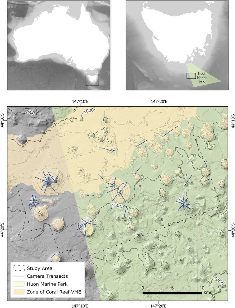
Figure 1. Bathymetric map showing location of the Tasmanian seamounts on the continental slopes of southern Tasmania, Australia. The study area, highlighted in the blue region on Map 3, is defined by an area where high resolution multibeam echosounder (MBES) data has been acquired. The area includes a subset of the Tasmanian seamounts totaling 77 seamounts, hills, and knolls. These are predominantly located within the Huon Marine Park, which is highlighted in green. Seafloor camera transects have been acquired over a portion of the seamounts, as highlighted by the blue lines. Bathymetry data from RV Investigator voyage in 2020_v10 and GEBCO 2023 Grid (2023). The depth range of 950–1,350 m, identified as the ‘Zone of Coral Reef VME,’ has been previously identified (Williams et al., 2020a).

Despite their ecological significance, seamount ecosystems are increasingly at risk due to growing pressures from human activities and environmental changes (Rogers, 2019). Bottom trawl fishing, in particular, has emerged as one of the most destructive forces affecting seamount ecosystems, with documented long-lasting impacts (Goode et al., 2020). A stark example of this damage was observed by Althaus et al. (2009), who recorded a dramatic reduction in coral cover and biodiversity on trawled Tasmanian seamounts. While the amount of coral removed from the seamounts as by-catch is unknown, nearby seamounts on the South Tasman Rise reported 1–15 tons of coral by-catch in individual trawls during the 1997–1998 fishing season (Althaus et al., 2009). Notably, Williams et al. (2010) found no signs of recovery even a decade after trawling had ceased, highlighting the vulnerability of these ecosystems. Compounding direct anthropogenic impacts, climate-related threats such as ocean acidification and warming further exacerbate the vulnerability of seamount ecosystems (Anderson et al., 2022), emphasizing the urgent need for robust conservation management strategies.

To develop and implement effective conservation strategies, it is crucial to understand the past, present and future distribution of seamount benthic communities (Stephenson et al., 2023). This knowledge is essential for identifying priority areas for protection, assessing potential impacts of human activities, and designing networks of marine protected areas that can ensure the long-term preservation of these ecologically significant habitats (Williams et al., 2010). However, the vast expanse and inaccessibility of the deep sea present significant challenges for conducting comprehensive ecological assessments of these complex ecosystems (Ramirez-Llodra et al., 2011).

In response to these challenges, researchers are increasingly turning to predictive species distribution modelling (SDM) as a tool to map and understand seamount ecosystems (Lim et al., 2020). SDMs offer a cost-effective approach to predict the potential distribution of species or habitats across large, unexplored areas based on known occurrences linked to environmental variables (Elith and Leathwick, 2009). While these models have proven useful in conservation management (Guisan et al., 2013), developing accurate and reliable SDMs for deep-sea ecosystems presents numerous difficulties, the main ones being data limitations and the complexity of these environments (Araújo et al., 2019).

Regional-scale SDMs, at resolutions of 500–1,000 m, have proven valuable for predicting the distribution of deep-sea species and habitats across large areas (Guinotte and Davies, 2014; Anderson et al., 2016b; Georgian et al., 2019). These models provide important insights for conservation planning and fisheries management; however, their reliability is often limited by the resolution of available environmental data (Winship et al., 2020) and the absence of crucial predictor variables (Anderson et al., 2016a). A significant ongoing challenge for regional-scale models is the lack of substrate information, which is critical for accurately predicting the distribution of benthic species. For example, Anderson et al. (2016b) attributed the poor performance of their regional models, as assessed through field validation (Anderson et al., 2016a), to a lack of substrate data. Similarly, Guinotte and Davies (2014) explicitly noted that their regional models likely overpredicted actual coral distribution due to the absence of data on hard substrate distribution. The importance of substrate type as a predictor of species distribution has also been repeatedly highlighted in best practice reviews of species distribution modelling (Bowden et al., 2021).

Additionally, the coarse resolution of regional models often fails to capture the fine-scale habitat heterogeneity characteristic of seamount ecosystems. This limitation can lead to significant overestimation of suitable habitat areas, as demonstrated by Williams et al. (2020a) in their study of Tasmanian seamounts. Their findings revealed that coral reef patches were substantially smaller (0.02–0.16 km²) than predicted by regional models, underscoring the need for higher-resolution approaches in areas of immediate conservation concern. Similarly, Rowden et al. (2017) and Goode et al. (2021) demonstrated the importance of fine-scale studies in understanding intra-seamount community dynamics.

The ability to model seamount ecosystems on a fine scale (at grid resolutions <25 m) has historically faced challenges similar to those encountered in regional-scale studies, particularly regarding the availability of critical predictor variables at the appropriate scale. In the case of the Tasmanian seamounts, two key factors have previously hindered the development of a comprehensive model: 1 the lack of detailed substrate information (Williams et al., 2020a) and 2 the absence of robustly quantified fishing impact data (Williams et al., 2020b).

In this study, we utilize a newly available high resolution acoustic backscatter data, together with the categorized fishing effort from Williams et al. (2020b), to predict distributions of VME habitat formed by S. variabilis over a subset of the Tasmanian seamounts. These data present the first opportunity to map patches of reef across a broad region (>480 km²) at a fine scale (15 m resolution), enabling multiple seamounts to be included in a single habitat suitability model. Our approach includes two distinct models. Model 1 predicts the current ‘VME habitat’ distribution based on an image-derived observational dataset analysed against fine-scale environmental data derived from multi-beam acoustics, including backscatter and an index of bottom trawling impact as a predictor variable to all seamounts; Model 2 predicts pre-impact ‘VME habitat’ based the same dataset, but excluding trawling impacts by removing both, the bottom trawling impact index predictor, and the observations on five seamounts known to have been heavily impacted by bottom trawling. This multi-model approach allows for a comparison of past and present VME habitat distribution, building upon the knowledge of past impacts to identify the potential habitats in this region (Althaus et al., 2009; Williams et al., 2010; Williams et al., 2020b).

This study builds upon the growing body of work modelling deep-water corals (Rowden et al., 2017; Goode et al., 2021; Anderson et al., 2022; Stephenson et al., 2023) examining the temporal changes in distribution, assessing the influence of crucial predictor variables, and evaluating the implications of these findings for conservation management. Ultimately, this work aims to assist in informing the development of management strategies that account for the dynamic nature of these ecosystems and the complex interplay of natural and anthropogenic factors influencing their distribution.

2 Materials and methods

2.1 Study area

The Tasmanian seamounts are located on the continental slope to the south of Tasmania, Australia (Figure 1). They are clustered, with approximately 191 seamounts (Williams et al., 2020a) scattered over an area >700 km² (Heap and Harris, 2008). The seamount peaks range in depths from 570 to 2,400 m and with seamount basal areas ranging from 0.2 to ∼20 km² (Williams et al., 2020a). Based on their morphology and very sparse geological sampling, the seamounts are believed to be volcanic in origin, with formative mechanisms thought to possibly relate to the Balleny Mantle Plume (Exon et al., 1997) or Edge Driven Convection (Davies and Rawlinson, 2014).

Our study area (Figure 1) covers a subset of the Tasmanian seamounts, of which the majority are contained within the Huon Marine Park. The area is defined by the availability of high-resolution multibeam echosounder (MBES) data which covers approx. 486 km² and includes 66 small seamounts with elevations from 100–530 m, and 7 knolls and hills with elevations from 65–100 m. Peak depths of these seamounts range from 720–2,073 m.

2.2 Predictor variables

Predictor variables describe the conditions that influence the presence of VME habitat to be modelled. For this study, most predictor variables are derived from MBES data. An additional predictor variable describes past commercial demersal trawl fishing effort.

2.3 Multibeam echosounder data

Sonar data of the seafloor in the study area were acquired during voyages IN2020_V10 and IN2021_V03 aboard Australia’s Marine National Facility vessel, the RV Investigator, using a Kongsberg EM122, a 12 kHz multibeam echosounder system. Line acquisition was optimized to ensure sufficient overlap between swath coverages, thus reducing the nadir artefacts in backscatter data and enhancing the overall resolution of resulting datasets (Figure 2). The products derived from these surveys included bathymetry and backscatter. Here, bathymetry refers to the gridded product in which each cell represents depth (meters). Backscatter refers to the gridded product in which each cell represents acoustic backscatter intensity (decibels).

Figure 2

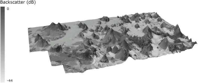
Figure 2. 3D perspective view of the study region showing segmented multibeam sonar backscatter overlaid on bathymetry with a vertical exaggeration of 3. Backscatter denotes acoustic backscatter intensity (dB) as recorded by a MBES and is used here as a substrate proxy. Backscatter segments delineate acoustically similar patches from which the predictor ‘Backscatter’ was derived.

Bathymetry data were processed using Caris HIPS and SIPS 11.4.12. Outliers in the data were removed, and a 15 m gridded CUBE surface was produced. This surface was imported into ArcGIS Pro v3.0.3 where Benthic Terrain Modeler and SAGA Toolbox add-ins were used to produce a suite of bathymetry-derived variables known to be useful in modelling deep-sea taxa (Rengstorf et al., 2012; Downie et al., 2021). As in previous studies, for example, Rowden et al. (2017), additional variables were derived by performing focal mean analysis of the input variables to produce more generalized data, allowing for the effect of scale to be examined. This process involves using a near-neighbor approach. Neighborhood sizes of 3 × 3, 5 × 5, 7 × 7 and 15 × 15 were utilized resulting in the production of over 100 predictor variables (Supplementary Table S1).

Backscatter data were processed with QPS Fledermaus Geocoder Toolbox (FMGT) 7.10.2 using beam time series and processing parameters set to flat AVG correction and a window size of 300. A mosaic with a 15 m resolution was produced and then imported to ArcGIS Pro v3.0.3 for segmentation. Segmentation is a process where pixels with similar characteristics are grouped together (Che Hasan et al., 2012; Misiuk and Brown, 2022). A mean shift segmentation algorithm was used in ArcGIS Pro, allowing adjustments to spatial, spectral, and segment size settings to meet user needs (Comaniciu and Meer, 2002). A maximum spectral setting and minimal spatial setting with a segment size of 100 pixels were used. These settings maximised the apparent heterogeneity of segments relative to the mosaic’s resolution. Segments were then used to calculate a mean backscatter value (dB) for each segment. The resulting raster was used as a substrate proxy with higher values typically indicating rock/coarse sediments and lower values finer/soft substrates (Lurton and Lamarche, 2015).

A categorical variable describing the footprints of individual seamounts was derived from bathymetry data using an approach that involved delineating the slope break from the normalized slope and normalized profile curvature (Grosse et al., 2009). This variable has been found useful for separating seamounts, based on variable specificity (Rowden et al., 2017).

2.4 Spatial representation of bottom fishing effort and impact

The study area includes seamounts exposed to commercial demersal trawling, particularly targeting orange roughy (Hoplostethus atlanticus). The trawl effort footprint overlaps the core range of S. variabilis with the most intensively trawled features showing great reductions in VME habitat (Williams et al., 2020b). The effects of this fishing are expected to be long lasting, with no observed recovery over a 10–year period following the cessation of trawling (Williams et al., 2010). While the impacts of bottom trawl fishing are typically not considered in modelling deep-ocean habitats, recent studies (Stephenson et al., 2023) have highlighted the significant impact it can have on model outputs.

The impacts of commercial demersal trawl fishing in the study site have previously been quantified and categorized (Williams et al., 2020b) to classify seamounts into four categories based on fishing impact on VME habitat: Heavily Impacted, Moderately Impacted, Lightly Impacted, and No Observed Impact; a fifth category of Off-Seamount was assigned to slope areas between seamount bases. The classification system used datasets including direct observation of impact (through camera surveys), locations of known trawl blocks, historical fishing data and known fishery depth range (<1,350 m). This classification system adopted a conservative approach to minimize the risk of false-positive classification of fishing impact. These impact classifications were appended to the ‘seamount’ categorical variable, where off-seamount values were retained, and impact indexes from ‘No Observed Impact’ to ‘Heavily Impacted’ were appended to individual seamounts.

In our study area, seamounts that were not assessed as part of the previous study by Williams et al. (2020b), highlighted as ‘Recoded’ in Figure 3, were classified based on proximity to fishing impacts, location on transit routes between impacted seamounts and naming of seamounts by the fishing industry.

Figure 3

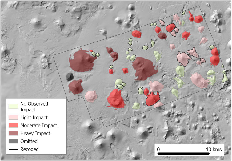
Figure 3. Commercial demersal trawl fishing impact classifications (Williams et al., 2020b). Four categories are used to classify fishing effort on seamounts: no observed impact, low impact, moderate impact and heavy impact. Areas between seamount bases were classified as ‘off-seamount.’

Due to anomalous observations on a seamount at the western end of the site (Figure 3, refer to ‘Omitted’), the footprint of this seamount was omitted from the fishing impact predictor variable and corresponding sonar derived predictor variables. Observations over this seamount were considered anomalous due to the high levels of VME habitat remaining, despite moderate levels of fishing effort.

2.5 Response variable

To predict the distribution of benthic taxa, a sample of locations where the taxa are present must be observed. These data, known as the response variable, informs the modelling process by indicating the taxa’s presence relative to predictor variables. The response variable used in this study is the presence/absence of VME habitat formed by S. variabilis. This response variable was derived from seabed imagery.

Seabed imagery was collected during the IN2018_V06 voyage aboard Australia’s Marine National Facility vessel, the RV Investigator, using a towed camera system. This system included a Canon EOS-1DX video camera for HD video and two Canon EOS-1DX Mark II cameras for stereo still images, viewing the seafloor at an oblique angle. The camera system was towed at a speed of 1 knot at an altitude of 2 m (±0.5 m) above the seafloor, with a Sonardyne Ranger 2 USBL system enabling georeferenced logging of the cameras and associated imagery.

Towed camera transects were planned employing a flexible, spatially balanced design (Foster et al., 2020). Three transect design approaches were employed: 1 Randomized Radial, 2 Randomized Baseline, and 3 ad hoc transects conducted during transits. Each transect was typically 2 km in length.

The resulting imagery was annotated using the Monterey Bay Aquarium Research Institute Video Annotation and Reference System (VARS). Reef cover was determined to represent a VME habitat by Williams et al. (2020a), following a method and criterion first described by Rowden et al. (2017): 25% coral reef cover with at least one live coral head in a moving window with a ratio of 3:5. This method provides a robust determination of coral cover relative to the definitions of VMEs.

Due to the anomalous nature of the observations on the seamount at the western end of the site (Figure 3 refer to ‘Omitted’) data from this location were omitted from the response variable. These observations were considered anomalous due to the high levels of remaining VME habitat, despite the known moderate levels of fishing impact.

2.6 Variable selection

Including redundant variables during the modeling process can lead to overfitting, which reduces the accuracy of predictions. Therefore, model performance improves by using a small number of the most relevant variables (Huang et al., 2011).

The initial suite of over 100 variables (Supplementary Table S1), was reduced by removing variables that were highly correlated, an approach commonly used in SDMs (Anderson et al., 2016a; Rowden et al., 2017; Goode et al., 2021). A Pearson correlation coefficient was calculated in R v4.2.2, and variable pairs/sets with r > 0.75 were represented by a single variable, removing the rest from further analyses.

To further reduce the suite of variables, a preliminary Random Forest (RF) model was constructed using this reduced set of variables. Variable importance was assessed according to the mean decrease in accuracy (MSE) scaled to 100% (Georgian et al., 2019). This process highlighted 10 variables of the highest relevance (Table 1). These variables were further examined in an additional Pearson correlation coefficient matrix which highlighted the low correlation of the remaining variables, as demonstrated by values of r < 0.75 (Figure 4) except for the Seamount and Fishing Impact variable. While the Seamount and Fishing Impact variables were highly correlated, they were not both used in the same model so were retained.

Table 1

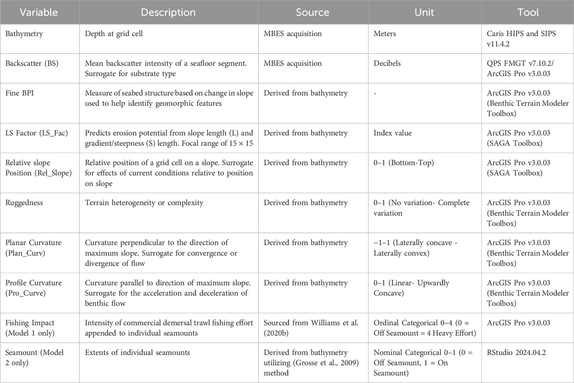
Table 1. The final set of variables utilized in modelling following the variable selection processes.

Figure 4

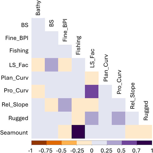
Figure 4. Pearson correlation coefficients of the least correlated variables. Removing highly correlated variables improves model performance. Variables with a correlation coefficient of >0.75 were not used although seamount and fishing effort which were retained and used in separate models. Variable abbreviations are given in Table 1.

2.7 Model selection and parameters

A Random Forest (RF) modelling approach (Breiman, 2001) was used to predict the spatial distribution of VME habitat formed by the coral S. variabilis.

RF models calculate habitat suitability using classification, or regression, trees (CART). CARTs examine the relationship between response and predictor variables by carrying out recursive binary splits of random subsets, or bootstraps, of training data (Strobl et al., 2009). Individual CARTs can have high variance, so ensembles of CARTs are utilized to provide a more generalized prediction (Hastie et al., 2009).

A RF approach was adopted due to its strong performance in previous studies (Du Preez et al., 2016; Rowden et al., 2017; Georgian et al., 2019; Goode et al., 2021), and due to its inbuilt model performance and variable assessment metrics. The RF model was developed using the R package “randomForest” (Liaw and Wiener, 2001).

Two models were developed to assess the past and present extent of VME habitat across the seamounts in the study area. Model 1 incorporated all predictor variables excluding the seamount variable (nine predictor variables) and the entire response variable dataset. This model provides a conservative prediction of current probability of presence accounting for the impacts of commercial demersal trawl fishing. In Model 2 observations from seamounts classified as ‘heavily impacted’ were excluded, observations from lightly and moderately impacted seamounts were retained, and the Fishing Impact predictor was removed, instead including the Seamount variable. This configuration limits the risk that disturbance-driven absences on heavily impacted seamounts are encoded as environmental limits, or false negatives, while retaining lightly and moderately impacted seamounts provides environmental contrasts under limited disturbance that help reduce false positives. Retaining these sites also maintained environmental variance and sample size for stable model estimation. Model 2 therefore provides a conservative, lower-bound VME habitat prediction of pre-impact conditions suitable for extrapolation across the region.

The hyperparameter ‘mtry’ was tuned for each model using the tuneRF function in the randomForest package with values of 4 for both models. The optimal value for ntree was determined through establishing the rate at which errors stabilized in initial models, found to be 1,500 and 1,000 for Model 1 and 2, respectively. As classification trees are sensitive to class imbalances a down sampling approach (Valavi et al., 2021) was used to balance the dataset.

2.8 Model performance

Model performance was evaluated based on assessments of area under the receiver operating characteristic curve (AUC) and True Skill Statistics (TSS) which were calculated through spatial block cross-validation.

AUC is a threshold independent model performance metric involving the comparison of a model’s predicted probabilities to withheld data across all possible thresholds, providing a single metric of discrimination (Fielding and Bell, 1997). The calculated AUC statistics range from 0–1 with AUC values greater than 0.5 indicating better than random performance, values 0.7–0.8 indicating adequate performance, and values greater than 0.8 indicating excellent performance (Hosmer et al., 2013).

TSS is a threshold dependent model performance metric which compares sensitivity (true prediction of presence) and specificity (correct prediction of absence). The calculated TSS statistics range from −1 – +1 where −1 indicates no better than random performance, and +1 indicates perfect performance with values of >0.6 considered to be useful (Allouche et al., 2006).

Performance metrics were calculated through spatial block cross-validation (Valavi et al., 2019). This approach accounts for spatial structuring where observations taken at geographically nearby locations are correlated (Tobler, 1970). Spatial structuring may result in overinflated assessment of model performance (Roberts et al., 2017) and is overcome by partitioning data into blocks with similar geographic locations. The block sizes used in cross-validation were calculated through assessment of the spatial autocorrelation in model residuals (Telford and Birks, 2009). Blocks were allocated to 1 of 10 folds, with each model being run 10 times to calculate mean AUC and TSS values.

2.9 Model uncertainty

Model uncertainty was evaluated by calculating the coefficient of variation (CV) for each cell in the prediction grid, following the methodology of Georgian et al. (2019) and Rowden et al. (2017). The CV is a measure of relative variability, calculated as the ratio of the standard deviation to the mean. For each cell, the CV was determined using 200 model iterations. To enhance interpretability, the CV for each cell was then expressed as a percentage.

Converting the CV to a percentage makes it easier to understand and compare the level of uncertainty across different cells by providing a clear, standardized measure of variability relative to the mean, which can be intuitively understood as the amount of variation per 100 units of the mean value.

2.10 Predictor variable influence

The importance of each predictor variable was assessed using the randomForest package’s inbuilt variable importance assessment. This method evaluates importance through permutation, calculating the mean decrease in accuracy (Liaw and Wiener, 2001). The relative influence of variables on class response was assessed utilizing partial dependence plots (PDP). PDPs indicate the average vote percentage for the class response across the range of the predictor variable, allowing for the analysis of the range for which the predictor variable contributes to class probability. The use of PDPs is particularly effective with RF models (Greenwell, 2017).

2.11 Model outputs and analysis

Outputs from each model included probability and uncertainty. These outputs were gridded at the resolution of the input data (15 m grid cells). The probability outputs represent the overall probability of the presence of VME habitat. Each cell within the output gives a value from 0–1 where 1 represents a high probability of VME habitat. The uncertainty output represents the uncertainty for each grid cell as represented by the percentage CV.

A comparison of predicted VME habitat area between models was made by applying a range of thresholds to probability outputs. Thresholds from 0.5–1 were utilized to calculate areas, in km², with the difference in areas between models providing an indication in changes in habitat extents. VME habitat patch sizes were directly compared using the threshold of 0.7 to define areas of highly probable presence (Stephenson et al., 2023).

The spatial disparity in predictions from Model 1 and 2 was assessed by calculating the differences between probability outputs. A difference surface was computed by subtracting values of one probability output from another.

To assist in the interpretation of predictions, the mean values of each predictor variable (excluding ‘Fishing Impact’ and ‘Seamount’) associated with each seamount footprint were computed.

These analyses were undertaken in ArcGIS Pro (v3.0.3).

3 Results

3.1 Model performance

To evaluate model performance while accounting for spatial autocorrelation, spatial block cross-validation was applied (Valavi et al., 2019), with block sizes determined by the range of spatial autocorrelation in model residuals. The resulting block sizes were 152 m for Model 1 and 222 m for Model 2, equating to approximately 10 and 15 grid cells respectively at the 15 m resolution of the environmental predictors. These relatively small block sizes indicate that spatial autocorrelation in residuals was confined to fine spatial scales, likely reflecting the influence of local environmental variation on species distributions. Model performance metrics were consistent across both models with excellent model performance, indicated by AUC values >0.94 (Hosmer et al., 2013; Table 2). TSS values >0.8 also support the usefulness of modelling outputs (Allouche et al., 2006). These consistently strong results align with the performance of RF models in other studies (Rowden et al., 2017; Georgian et al., 2019).

Table 2

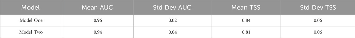
Table 2. Model performance metrics as assessed by spatial block cross-validation.

3.2 Predictions of coral VME distribution

Strong performance by both models was also supported by a high predicted probability of coral VME habitat within the coral zone, within the seamount footprint and on seamount peaks, i.e., generally consistent with previous observations (see Williams et al., 2020b) (Figures 5A,C, for Model 1 and Model 2, respectively).

Figure 5

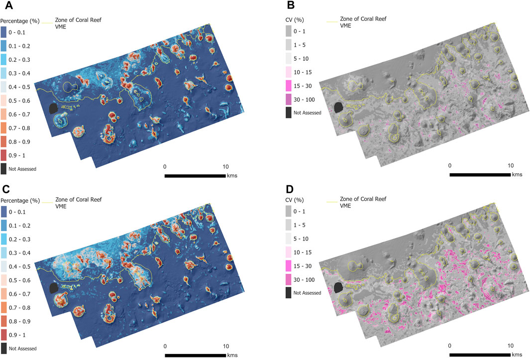
Figure 5. The predicted probability of VME habitat (0%–100%) and Uncertainty of predictions (CV (%)) on the Tasmanian seamounts within the study site for Model 1 (A, B) and Model 2 (C, D).

A map of prediction uncertainty indicated that all areas with a high probability (>50%) of coral VME habitat presence, identified in both models, were associated with low uncertainty (<10%) (Figures 5B,D, for Model 1 and Model 2, respectively). In contrast, regions with relatively high uncertainty were located off seamounts and in deeper parts of the site, beyond the typical depth range of VME habitat formed by S. variabilis.

The most notable between-model differences in the predicted distributions of coral VME occurred on the seven heavily trawled seamounts (Figure 6: seamount 1–7) where Model 2 (before trawling) predicted substantially larger suitable VME habitat areas (Figure 6). Increased, but relatively smaller, VME habitat areas were apparent on several lightly trawled seamounts (Figure 6: seamount 22–30) Between-model differences on moderately trawled seamounts (Figure 6: seamount 8–21) were minimal. Unimpacted seamounts also showed little to no difference between models.

Figure 6

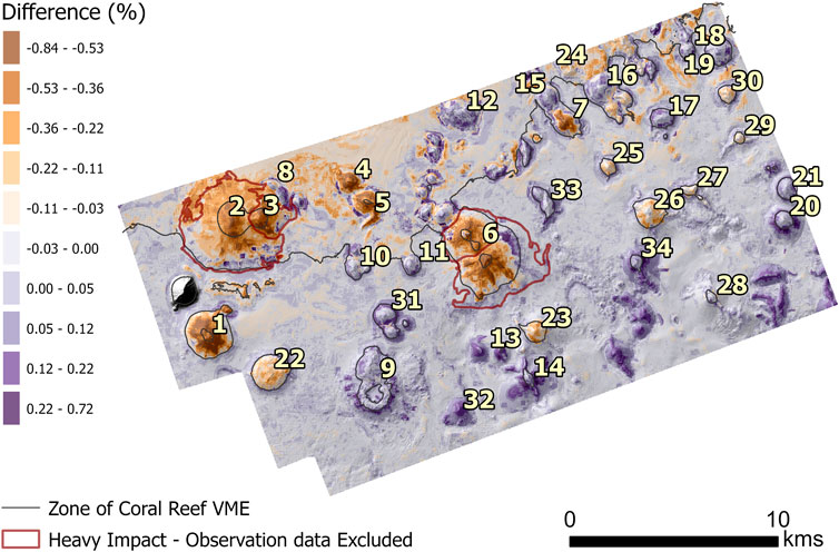
Figure 6. The difference in probability of predicted presence between Model 1 and Model 2. Seamount numbers utilized for identification purposes in analysis of results. Heavily impacted seamounts where observation data were excluded are also shown.

3.3 Predictions of coral VME area

The total area of suitable VME habitat predicted by each model was compared using a range of probability thresholds from 0.5–1. Model 1 (including trawling impact) consistently predicted smaller areas of suitable VME habitat than Model 2 (excluding trawling impact) (Figure 7). At a threshold of 0.5, the total area of VME habitat predicted by Model 1 was 29.40 km², while Model 2 predicted a total area of 39.77 km². In both cases, the total area of suitable VME habitat declined as the threshold increased to 1.0 (probability = certain).

Figure 7

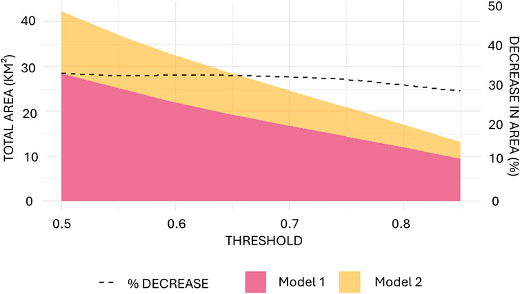
Figure 7. Differences in total predicted VME habitat area based on thresholds from 0.5–0.8 (C).

A decrease in VME habitat area of 20.44%–26.07% following trawling was predicted across the range of probability thresholds from 0.5–0.85. However, as thresholds increased above 0.80, the difference narrowed significantly, with Model 1 predicting 14.7%–14.3% less habitat than Model 2 for thresholds between 0.8 and 0.9. Using a probability threshold of 0.7 (Stephenson et al., 2023), Model 1 predicted VME habitat patch sizes up to 0.91 km² and a total area of 18.06 km² (Figure 8A). Model 2 predicted patch sizes up to 1.37 km² and a total area of 22.50 km² (Figure 8B).

Figure 8

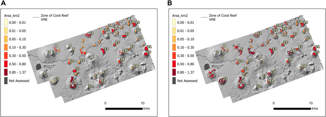
Figure 8. (A) The predicted VME habitat patch sizes from Model 1 based on a threshold of 0.7. Seamount numbers utilized for identification purposes in analysis of results. (B) The predicted VME habitat patch sizes from Model 2 based on a threshold of 0.7. Seamount numbers utilized for identification purposes in analysis of results.

The largest predicted loss of VME habitat was observed on the heavily fished seamount 1 (Figure 6). Model 1 predicted an almost complete loss of VME habitat on this seamount, with three significant patches being predicted as removed when using a threshold of 0.7 (Figure 8A). On the other large, heavily fished seamounts (Figure 6: seamounts 2,3,6) only very small patches of VME habitat (<0.01) were predicted with Model 1. Model 2 predicted only relatively small dispersed VME habitat patches on seamounts 2,3,6.

Lightly fished seamounts were consistently predicted to have decreased habitat after trawling, with seamount 22 showing the highest VME habitat loss. This seamount supported the second largest contiguous habitat patch (1.18 km²) in Model 2 when using a threshold of 0.7. In Model 1 this large contiguous patch was reduced to over 60 small patches from 0.001–0.09 totaling 0.43 km².

Moderately impacted seamounts exhibited minimal differences between models, with only slight decreases or increases in VME habitat area. Slight decreases in VME habitat area were predicted (∼0.05 km² at a threshold of 0.7) on several smaller seamounts (8, 14, 20) while seamounts 10 and 21 saw no change in area. Slight increases of 0.04–0.13 km² (at a threshold of 0.7) were observed on seamounts 11, 12, 13, 15, 16, 17, 18, 19, 20. Seamount 9, the largest moderately fished seamount, contained the largest contiguous VME habitat patch in Model 1. In Model 2, this area decreased by 0.17 km². This decrease in VME habitat from Model 1 to Model 2 accounts for 0.7% of the total area and thus has minimal impact on the overall indications of changes in area. Accounting for the minor increases observed on several moderately fished seamounts, the results likely underestimate the overall reduction in coral cover caused by fishing impacts.

3.4 Predictor variable influence

Bathymetry was the most influential predictor variable in both models (Table 3), with a strong positive correlation between the 950–1,350 m depth range and higher coral VME habitat probability (Supplementary Figures S1, S2). The exclusion of the fishing impact variable in Model 2 resulted in an increase in the relative importance of bathymetry, indicating its strong predictive value for VME habitat distribution. Fishing impact was highly influential in Model 1 (Table 3) and was negatively correlated with VME habitat probability in heavily fished areas. Lightly fished areas also exhibited a reduced probability of VME habitat, whereas moderately fished areas showed similar probability between models.

Table 3

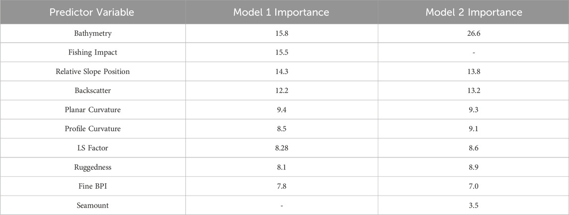
Table 3. Predictor variable importance for Model 1 and Model 2.

Terrain complexity played a key role in habitat predictions. Relative slope position showed a near-linear correlation with VME habitat probability in both models (Supplementary Figures S1, S2), with increasing values (closer to 1) indicating a preference for areas near seamount peaks. Ruggedness also contributed positively, with more structurally complex terrain associated with higher VME habitat probability. Terrain on the most heavily impacted seamounts exhibited lower mean profile curvature (i.e., flatter slopes; 0.035–0.036, Supplementary Figure S8) and reduced ruggedness (0.0002–0.0009, Supplementary Figure S10), which may reflect: 1 a loss of fine-scale structural complexity due to trawling; 2 the contribution of VME habitat itself to seafloor complexity; or 3 an inherent lack of structural complexity that made these areas more attractive to fishers. LS Factor, an index of erosion potential that increases with slope steepness and length, was positively correlated with VME habitat probability up to a value of 50. Above this threshold, habitat probability declined in Model 2 but remained stable in Model 1, possibly reflecting contrasting sensitivities to substrate stability and sediment dynamics. Curvature metrics also influenced predictions: profile curvature values around 0.05 — indicative of convex slopes where flow is accelerating—were associated with higher habitat probability, while planar curvature values near 0 — representing flat or linear terrain with minimal convergent or divergent flow—were linked to lower habitat probability. In summary, the most suitable locations for coral VME habitat were the complex, rugged, and steep terrains of seamount flanks near their peaks.

Backscatter emerged as a significant predictor variable in both models (Table 3). A positive correlation was observed between backscatter values approaching −32 dB (Supplementary Figures S1, S2) and VME habitat probability. Probability sharply decreased as backscatter values moved away from ∼ −32 dB, indicating that this range represents an optimal substrate condition. The largest and most heavily impacted seamounts (Figure 6: seamounts 2, 3, 6) exhibited distinctly higher mean backscatter values (−26.1 dB ± 0.24) compared to other heavily impacted seamounts (−29.5 dB ± 3.3), moderately impacted (−29.3 dB ± 2.2), lightly impacted (−28.8 dB ± 2.7), and unimpacted areas (−29.9 dB ± 3.3). These patterns suggest potential differences in seafloor characteristics between heavily fished and less impacted areas.

4 Discussion

4.1 The influence of predictor variables

The varying availability and resolution of environmental predictor variables for benthic fauna has a strong and often unknown impact on the performance and reliability of model outputs (Bowden et al., 2021). Those that influence the distribution of VME habitat forming deep-water corals have been well-described, although they may be unavailable, or have diminished value following data cleaning to an appropriate accuracy and/or spatial resolution when they will hinder even the most sophisticated modelling efforts (Bowden et al., 2021). Models that lack important environmental predictor variables have been found to provide unreliable predictions (Anderson et al., 2016a) and thereby limit their utility for conservation management planning. Our analysis of the Tasmanian seamounts, a relatively well-surveyed area (Williams et al., 2020a), has generated the best set of critical predictor data (such as precise backscatter measurements) to enable robust fine-scale modelling.

Overall, the variable that most strongly influenced the prediction of VME habitat was bathymetry; the highly correlated depth range (950–1,350 m) aligned tightly with the core depth ranges of S. variabilis documented at this location by several studies (Williams et al., 2020a). Our bathymetry data were more finely resolved than in historical studies (15 vs. ≥ 40 m grid), and therefore better suited to the model based on video transect-derived VME distribution mapped at ∼25 m² patch resolution (∼12 m long × 2 m plan view wide), and the spatial scale of variation of patches where coral VME was sparse (Williams et al., 2020a). This finer resolution was likely critical for capturing the small-scale topographic complexity of seamount flanks and peaks—such as local ridges, ledges, and abrupt slope transitions—which are often obscured in coarser-resolution datasets (Georgian et al., 2019). It also enabled the detection of discrete habitat patches across the study area, with predicted patch sizes ranging from <0.01 km² to a maximum of 1.37 km², — exceeding the largest patch (1.16 km²) previously reported (Williams et al., 2020a). Across a growing body of habitat modelling literature, bathymetry and its derivatives consistently emerge as dominant predictors of deep-sea coral and benthic community distributions (Du Preez et al., 2016; Rowden et al., 2017; Goode et al., 2021). These variables serve as effective proxies for underlying environmental gradients, such as hydrodynamic energy, substrate type, and food availability, especially in data-limited deep-sea settings (Downie et al., 2021). The strong influence of bathymetry and terrain metrics in our models aligns with these previous studies and further supports the central role of fine-scale topographic structure in shaping the distribution of habitat-forming corals on seamounts.

Significant fishing impacts have been observed across the study site (Althaus et al., 2009) and have been comprehensively described, quantified, and extrapolated in a previous study (Williams et al., 2020b). In this study, fishing impact data were incorporated into Model 1, where it emerged as an influential variable. Specifically, areas classified as having ‘Heavy’ fishing impact were associated with significant reductions in predicted coral presence compared to Model 2. The strong influence of the fishing impact variable aligns with recent findings (Stephenson et al., 2023), which highlight the critical role such data play in predicting species distributions.

The inclusion of trawling impact data in Model 1 resulted in consistently lower predicted VME habitat area across a range of probability thresholds. These differences were most pronounced on heavily fished seamounts, where Model 1 predicted almost complete loss of suitable VME habitat. The effect was less pronounced on lightly and moderately fished seamounts, though reductions in predicted habitat area were still observed. On moderately fished seamounts, where habitat cover differed only marginally between models, localized increases in predicted habitat were observed in some areas, despite an overall decline. This highlights the nuanced influence of fishing pressure on VME habitat where impacts may vary depending on historical fishing intensity and local environmental conditions.

Incorporating trawling impacts is essential for understanding coral VME distributions in this region, but quantifying fishing effects at scales comparable to high-resolution sonar-derived variables poses considerable challenges. The fishing impact data used here were at a broader spatial scale than the bathymetric and backscatter data, potentially introducing uncertainty into the model outputs (Vierod et al., 2014). Despite this discrepancy, Pittman and Brown (2011) demonstrated that integrating broad-scale variables with fine-scale data can enhance model performance, underscoring the value of combining datasets. However, the coarser resolution of the fishing impact variable in this study may limit its ability to detect fine-scale variations in fishing pressure, potentially obscuring localized areas of higher or lower impact within the broader classified zones. This limitation suggests that while the model effectively captures broad-scale habitat changes, localized impacts may require finer-resolution fishing effort data to improve predictive accuracy.

Substrate type is a key factor influencing the distribution of deep-water corals that form VMEs, yet it is often missing from predictive models due to a lack of high-quality, spatially consistent data (Anderson et al., 2016b; Georgian et al., 2019; Anderson et al., 2022). Substrate may be inferred from multibeam sonar backscatter (Lamarche et al., 2011), but only when acquisition follows defined standard operating procedures to ensure data quality (Przeslawski et al., 2019). In this study, acoustic backscatter was included in both models and had a relatively strong influence on VME predictions. A backscatter value of approximately −32 dB (Supplementary Figures S1, S2) was associated with higher probabilities of VME habitat, with a sharp decline in suitability observed at values above and below this threshold.

In general, lower backscatter values (more negative dB) are associated with soft sediments such as mud or fine sand, while higher values (less negative) indicate harder substrates like exposed rock or consolidated reef. The peak at −32 dB likely reflects intermediate substrate conditions—such as coarse gravel, mixed sediment, or encrusted surfaces—which may offer both stability and microhabitat complexity for coral attachment. Interestingly, the highest backscatter values, which typically correspond to the hardest substrates, were not associated with the highest VME probabilities. This could appear counter-intuitive given that corals require hard substrate for attachment (Roberts, 2009). However, it may reflect a range of interacting factors, such as intense current scouring on bare rock, a lack of fine-scale heterogeneity, or even biological masking of the acoustic signal. Thick coral matrices themselves may attenuate or scatter the sonar return, effectively reducing the measured backscatter strength despite their presence on hard substrate beneath.

While backscatter thresholds appear useful for identifying suitable VME habitat, it is important to note that these values are relative; absolute interpretation would require sonar calibration (Lucieer and Lamarche, 2011). The importance of standardising backscatter acquisition and processing has been widely recognised. Lamarche and Lurton (2018) provide best-practice recommendations for improving coherence and comparability across systems. Schimel et al. (2018) also emphasised the need for calibration and consistent workflows to improve habitat assessments. Building on these principles, advanced acquisition and processing techniques, such as backscatter intensity normalization and oversampling, have proven effective in improving the resolution of seafloor features in deep-water environments (Mitchell et al., 2018). Their application using autonomous underwater vehicles (AUVs) has enabled high-resolution backscatter mapping in deep-ocean settings, helping to overcome the limitations of hull-mounted systems at depth. Incorporating similar AUV-based approaches into future VME studies could help better resolve fine-scale substrate complexity in structurally complex or rugose benthic environments, potentially improving the accuracy of predictive habitat models for VMEs in deep-ocean settings.

This study demonstrates how the integration of high-resolution bathymetry, backscatter data, and fishing impact information enhances our ability to model VME habitat distribution with greater accuracy. Bathymetry emerged as the strongest predictor of habitat presence, with its derivatives providing valuable proxies for environmental conditions such as water flow and current exposure (Walbridge et al., 2018). Backscatter data played a key role in identifying substrate characteristics, though its utility is dependent on the availability of standardized and calibrated datasets. The influence of fishing impact data was also evident, particularly in areas with heavy historical trawling, where significant habitat loss was observed. However, challenges remain in aligning fine-scale habitat models with coarser-resolution fishing data, emphasizing the need for improved spatial resolution in anthropogenic impact datasets. These findings reinforce the importance of incorporating ecologically meaningful environmental predictors into fine-scale modeling efforts (Rowden et al., 2017; Ramiro-Sánchez et al., 2019) to support deep-sea conservation and management strategies, particularly in regions where human activities continue to shape benthic ecosystems.

4.2 Past and present VME habitat extents

The distribution of coral VME habitat on the Tasmanian seamounts has been significantly impacted by historical commercial demersal trawl fishing, resulting in documented reductions in coral cover (Althaus et al., 2009) and seamount-scale estimates of impact severity across the regional seascape (Williams et al., 2020b). However, until now, no studies have quantified the spatial extent of VME habitat reduction due to a lack of necessary data. In this study, we provide an estimate for a sub-regional area where demersal trawling was concentrated, comparing model predictions for pre- and post-trawling conditions. This approach builds on international efforts to quantify habitat changes using predictive modeling (Davies and Guinotte, 2011; Stephenson et al., 2021; Gros et al., 2022).

Fishing impact was incorporated into Model 1, following classifications largely derived from Williams et al. (2020b), while Model 2 represented pre-trawling conditions by excluding observational data from heavily fished seamounts. Observations from moderately and lightly fished sites were retained to train the model; this was not ideal but was necessary because very few seamounts had experienced zero historical trawling. This therefore results in a conservative historical estimate of pre-trawling coral VME distribution by likely underestimating its extent in some areas where trawling impacts were not recognised.

Heavily trawled seamounts exhibited the most substantial declines in VME habitat, with Model 1 predicting near-complete loss on the largest impacted seamounts (Figure 6: seamounts 1–7). This is consistent with global patterns, where historically trawled seamounts have exhibited extensive habitat degradation (Clark et al., 2015; Rogers, 2018). On these heavily fished seamounts, Model 2 predicted only small patches of suitable habitat (<0.14 km²) near seamount peaks and flanks prior to fishing. The absence of coral rubble in previous seafloor observations at these sites further supports this result (Williams et al., 2020b) suggesting that environmental conditions, such as reduced terrain complexity, lower profile curvature, and differing substrate (indicated by higher backscatter values) may have been less favorable for the formation and persistence of VME habitat.

VME habitat fragmentation, as a result of trawling, was evident across the study area, with the most pronounced effects observed on the largest lightly fished seamount, seamount 22 (Figure 6). This seamount exhibited the greatest degree of fragmentation, where a contiguous patch of 1.18 km² in Model 2 (pre-trawling) was reduced to over 60 small patches (<0.09 km² each) in Model 1 (post-trawling). Model predictions suggest that even low levels of fishing activity can lead to significant habitat fragmentation, potentially reducing connectivity between coral communities. Such fragmentation has been identified as a factor limiting recovery potential for deep-sea coral ecosystems following trawling disturbance (Goode et al., 2020).

In contrast, seamounts classified as ‘Moderately’ impacted exhibited relatively high predicted VME habitat probabilities, often exceeding those of lightly fished or unimpacted seamounts. This likely reflects their initially high coral cover, which may have made them attractive targets for trawling activity. Interestingly, Model 2 (representing pre-trawling conditions) predicted slightly higher habitat coverage on moderately fished seamounts than Model 1 (post-trawling). While this might appear counterintuitive given their classification, it is likely a result of residual influence from high initial coral abundance in the model training data, which continued to drive predictions in both models. Thus, the apparent slight increase is not interpreted as a genuine expansion of habitat post-disturbance, but more likely an artefact of how remaining presence data influenced predictions. These results suggest that moderately impacted seamounts, despite experiencing some habitat loss, may still retain more suitable habitat than lightly fished seamounts, which were potentially less favorable for coral VME development even prior to trawling.

These results highlight the value of high-resolution habitat modeling for improving our understanding of the distribution and spatial configuration of coral VMEs on the Tasmanian seamounts. The comparison between pre- and post-trawling scenarios illustrates how fine-scale predictions can reveal shifts in habitat extent and fragmentation that may not be detectable at broader scales. The ability to identify small, spatially distinct patches of suitable habitat—often located on seamount flanks or ridge features—demonstrates the benefits of incorporating detailed bathymetric, substrate, and impact data into modeling efforts. These insights provide a stronger basis for spatial planning and resource management in complex deep-sea environments, and contribute to broader efforts to assess habitat change, resilience, and recovery potential over time.

4.3 Implications for environmental management

VME habitat forming deep-sea corals are highly vulnerable to anthropogenic disturbances, including bottom trawling (Clark et al., 2019), mining (Schlacher et al., 2014), and climate change (Roberts and Cairns, 2014). Given their slow growth rates, with reefs taking centuries or even millennia to develop (Fallon et al., 2014), these ecosystems require proactive and precautionary management approaches. In this context, fine-scale, spatially explicit habitat modeling offers a valuable tool for identifying ecologically significant or sensitive areas and supporting informed conservation efforts.

Broad-scale and high-resolution modeling approaches are particularly suited to informing detailed reserve design, especially at local and sub-regional scales where fine-scale habitat heterogeneity is most relevant (Gros et al., 2022). Models at this resolution align with global best-practice recommendations—including those of the Food and Agriculture Organization (FAO, 2009) —which emphasize the importance of applying the best available scientific information, including predictive models, to guide spatial closures and mitigation strategies. These approaches are also consistent with broader international frameworks such as the Convention on Biological Diversity and its Kunming-Montreal Global Biodiversity Framework, which targets the protection of 30% of marine areas by 2030.

In our study, the differences observed between the pre- and post-trawling model predictions highlight how historical demersal fishing activity may have influenced the present-day distribution of suitable coral habitat, a pattern also reported in other deep-sea regions (Clark et al., 2019; Goode et al., 2020). Within the study area, several seamounts showed reduced suitability in the post-trawling model, reinforcing the importance of integrating historical disturbance data into predictive frameworks when evaluating current habitat conditions and setting conservation priorities.

Importantly, the modeling framework developed in this study is scalable and adaptable. It provides a practical foundation for application in other data-limited deep-sea regions, particularly where multibeam bathymetry and other environmental datasets are available. As global initiatives such as the UN Decade of Ocean Science for Sustainable Development (Ryabinin et al., 2019) seek to enhance ocean knowledge and inform marine spatial planning, tools that integrate acoustic, ecological, and anthropogenic impact data at high spatial resolution will become increasingly relevant in helping to support adaptive and informed management responses.

Looking ahead, the continued development of high-resolution, spatially explicit models will be essential as deep-sea ecosystems face mounting pressures from industrial activity and climate-related stressors (Ramirez-Llodra et al., 2011). These models can enhance our ability to assess habitat connectivity, identify potential recovery areas, and refine conservation strategies in line with changing ocean conditions. VME-forming deep-sea corals act as biodiversity hotspots, supporting diverse benthic communities (Henry and Roberts, 2017; Williams et al., 2021; Maguire et al., 2023). Their persistence may also bolster the broader resilience of marine ecosystems (Thurber et al., 2014), particularly as species seek climate refugia in the face of ocean warming and acidification (Tittensor et al., 2010). Protecting these habitats through science-based, data-driven approaches will be critical to ensuring their long-term viability.

5 Conclusion

Modelling is increasingly being used to predict and understand the spatial patterns of biodiversity, particularly in the deep sea (Rowden et al., 2017; Georgian et al., 2019; Goode et al., 2021). However, SDMs still face significant challenges due to the lack of spatially explicit data, including fine-scale environmental data, data quantifying anthropogenic impacts, and the uncertainty in the temporal methods to predict species distributions over time. Despite these obstacles, our study highlights the utility of fine-scale modelling in capturing critical habitat features, such as VME habitat forming deep-water coral reef patches, and demonstrates the importance of incorporating both substrate information and fishing impacts into SDM predictions.

Our findings, which predict a reduction in VME habitat due to commercial demersal trawl fishing, emphasize the need to account for human impacts in biodiversity models. Although this estimate is likely conservative, and the actual loss of VME habitat may be higher, it offers a valuable baseline for guiding future management strategies. It also highlights the urgent need for more comprehensive assessments of how human activities affect deep-sea ecosystems.

To improve our understanding of deep-ocean ecosystems, high-resolution acoustic multibeam bathymetric and backscatter data and correlated seafloor imagery are critically needed. Initiatives like Seabed 2030 (Mayer et al., 2018), Seamap Australia (Lucieer et al., 2019) and AusSeabed (Townsend et al., 2023) are advancing efforts to provide accessible, high-quality seafloor mapping data adhering to FAIR data standards and incorporating internationally consistent classification models. Expanding on these efforts is essential, particularly through open access to substrate data, which is crucial for refining SDMs and informing more effective marine conservation strategies.

Data availability statement

The datasets presented in this study can be found in online repositories. The names of the repository/repositories and accession number(s) can be found in the article/https://doi.org/10.25919/knqv-2t21.

Author contributions

CB: Investigation, Software, Writing – review and editing, Resources, Validation, Writing – original draft, Data curation, Project administration, Methodology, Visualization, Formal Analysis. VL: Conceptualization, Writing – original draft, Funding acquisition, Writing – review and editing, Resources, Methodology, Project administration, Supervision. JW: Resources, Funding acquisition, Project administration, Writing – original draft, Conceptualization, Supervision, Writing – review and editing. FA: Methodology, Writing – review and editing, Data curation, Conceptualization. AW: Writing – review and editing, Methodology, Conceptualization, Investigation, Funding acquisition, Writing – original draft.

Funding

The author(s) declare that financial support was received for the research and/or publication of this article. Project data were collected during a voyage on Australia’s Marine National Facility Vessel, RV Investigator, funded through the Australian Government. Modelling, data analysis and writing were partially funded by CSIRO.

Acknowledgments

The authors wish to thank and acknowledge the support staff and marine crew aboard CSIRO’s RV Investigator (https://ror.org/01mae9353) for facilitating the data acquisition associated with this project. We also thank and acknowledge the many other engineering, technical and administrative staff at CSIRO who contributed to supporting the project that provided the data for this manuscript. We thank and acknowledge input and guidance on modelling from Nicole Hill, Skip Woolley and Jan Jansen.

Conflict of interest

The authors declare that the research was conducted in the absence of any commercial or financial relationships that could be construed as a potential conflict of interest.

Generative AI statement

The author(s) declare that no Generative AI was used in the creation of this manuscript.

Any alternative text (alt text) provided alongside figures in this article has been generated by Frontiers with the support of artificial intelligence and reasonable efforts have been made to ensure accuracy, including review by the authors wherever possible. If you identify any issues, please contact us.

Publisher’s note

All claims expressed in this article are solely those of the authors and do not necessarily represent those of their affiliated organizations, or those of the publisher, the editors and the reviewers. Any product that may be evaluated in this article, or claim that may be made by its manufacturer, is not guaranteed or endorsed by the publisher.

Supplementary material

The Supplementary Material for this article can be found online at: https://www.frontiersin.org/articles/10.3389/frsen.2025.1650603/full#supplementary-material

References

Allouche, O., Tsoar, A., and Kadmon, R. (2006). Assessing the accuracy of species distribution models: prevalence, kappa and the true skill statistic (TSS). J. Appl. Ecol. 43 (6), 1223–1232. doi:10.1111/j.1365-2664.2006.01214.x

CrossRef Full Text | Google Scholar

Althaus, F., Williams, A., Schlacher, T., Kloser, R., Green, M., Barker, B., et al. (2009). Impacts of bottom trawling on deep-coral ecosystems of seamounts are long-lasting. Mar. Ecol. Prog. Ser. 397, 279–294. doi:10.3354/meps08248

CrossRef Full Text | Google Scholar

Anderson, O. F., Guinotte, J. M., Rowden, A. A., Clark, M. R., Mormede, S., Davies, A. J., et al. (2016a). Field validation of habitat suitability models for vulnerable marine ecosystems in the South Pacific Ocean: implications for the use of broad-scale models in fisheries management. Ocean and Coast. Manag. 120, 110–126. doi:10.1016/j.ocecoaman.2015.11.025

CrossRef Full Text | Google Scholar

Anderson, O. F., Guinotte, J. M., Rowden, A. A., Tracey, D. M., Mackay, K. A., and Clark, M. R. (2016b). Habitat suitability models for predicting the occurrence of vulnerable marine ecosystems in the seas around New Zealand. Deep Sea Res. Part I Oceanogr. Res. Pap. 115, 265–292. doi:10.1016/j.dsr.2016.07.006

CrossRef Full Text | Google Scholar

Anderson, O. F., Stephenson, F., Behrens, E., and Rowden, A. A. (2022). Predicting the effects of climate change on deep-water coral distribution around New Zealand—will there be suitable refuges for protection at the end of the 21st century? Glob. Change Biol. 28 (22), 6556–6576. doi:10.1111/gcb.16389

PubMed Abstract | CrossRef Full Text | Google Scholar

Araújo, M. B., Anderson, R. P., Márcia Barbosa, A., Beale, C. M., Dormann, C. F., Early, R., et al. (2019). Standards for distribution models in biodiversity assessments. Sci. Adv. 5 (1), eaat4858. doi:10.1126/sciadv.aat4858

PubMed Abstract | CrossRef Full Text | Google Scholar

Bowden, D. A., Anderson, O. F., Rowden, A. A., Stephenson, F., and Clark, M. R. (2021). Assessing habitat suitability models for the deep sea: is our ability to predict the distributions of seafloor fauna improving? Front. Mar. Sci. 8, 632389. doi:10.3389/fmars.2021.632389

CrossRef Full Text | Google Scholar

Breiman, L. (2001). Random forests. Mach. Learn. 45 (1), 5–32. doi:10.1023/a:1010933404324

CrossRef Full Text | Google Scholar

Che Hasan, R., Ierodiaconou, D., and Laurenson, L. (2012). Combining angular response classification and backscatter imagery segmentation for benthic biological habitat mapping. Estuar. Coast. Shelf Sci. 97, 1–9. doi:10.1016/j.ecss.2011.10.004

CrossRef Full Text | Google Scholar

Clark, M. R., Althaus, F., Schlacher, T. A., Williams, A., Bowden, D. A., and Rowden, A. A. (2015). The impacts of deep-sea fisheries on benthic communities: a review. ICES J. Mar. Sci. 73 (Suppl. l_1), i51–i69. doi:10.1093/icesjms/fsv123

CrossRef Full Text | Google Scholar

Clark, M. R., Bowden, D. A., Rowden, A. A., and Stewart, R. (2019). Little evidence of benthic community resilience to bottom trawling on seamounts after 15 years. Front. Mar. Sci. 6, 63. doi:10.3389/fmars.2019.00063

CrossRef Full Text | Google Scholar

Comaniciu, D., and Meer, P. (2002). Mean shift: a robust approach toward feature space analysis. IEEE Trans. Pattern Analysis Mach. Intell. 24 (5), 603–619. doi:10.1109/34.1000236

CrossRef Full Text | Google Scholar

Davies, A. J., and Guinotte, J. M. (2011). Global habitat suitability for framework-forming cold-water corals. PLoS ONE 6 (4), e18483. doi:10.1371/journal.pone.0018483

PubMed Abstract | CrossRef Full Text | Google Scholar

Davies, D. R., and Rawlinson, N. (2014). On the origin of recent intraplate volcanism in Australia. Geology 42 (12), 1031–1034. doi:10.1130/g36093.1

CrossRef Full Text | Google Scholar

Downie, A.-L., Vieira, R. P., Hogg, O. T., and Darby, C. (2021). Distribution of vulnerable marine ecosystems at the South sandwich islands: results from the blue belt discovery expedition 99 deep-water camera surveys. Front. Mar. Sci. 8, 662285. doi:10.3389/fmars.2021.662285

CrossRef Full Text | Google Scholar

Du Preez, C., Curtis, J. M. R., and Clarke, M. E. (2016). The structure and distribution of benthic communities on a shallow seamount (cobb seamount, northeast pacific ocean). PLOS ONE 11 (10), e0165513. doi:10.1371/journal.pone.0165513

PubMed Abstract | CrossRef Full Text | Google Scholar

Elith, J., and Leathwick, J. (2009). Species distribution models: ecological explanation and prediction across space and time. Annu. Rev. Ecol. Evol. Syst. 40, 677–697. doi:10.1146/annurev.ecolsys.110308.120159

CrossRef Full Text | Google Scholar

Exon, N. F., Berry, R. F., Crawford, A. J., and Hill, P. J. (1997). Geological evolution of the east tasman plateau, a continental fragment southeast of Tasmania. Aust. J. Earth Sci. 44 (5), 597–608. doi:10.1080/08120099708728339

CrossRef Full Text | Google Scholar

Fallon, S. J., Thresher, R. E., and Adkins, J. (2014). Age and growth of the cold-water scleractinian Solenosmilia variabilis and its reef on SW Pacific seamounts. Coral Reefs 33 (1), 31–38. doi:10.1007/s00338-013-1097-y

CrossRef Full Text | Google Scholar

FAO (2009). International guidelines for the management of deep-sea fisheries in the high-seas. Rome: Food and Agriculture Organisation of the United Nations.

Google Scholar

Fielding, A. H., and Bell, J. F. (1997). A review of methods for the assessment of prediction errors in conservation presence/absence models. Environ. Conserv. 24 (1), 38–49. doi:10.1017/s0376892997000088

CrossRef Full Text | Google Scholar

Foster, S. D., Hosack, G. R., Monk, J., Lawrence, E., Barrett, N. S., Williams, A., et al. (2020). Spatially balanced designs for transect-based surveys. Methods Ecol. Evol. 11 (1), 95–105. doi:10.1111/2041-210x.13321

CrossRef Full Text | Google Scholar

GEBCO (2023). GEBCO compilation group. Available online at: https://www.gebco.net/data-products/gridded-bathymetry-data/gebco2023-grid doi:10.5285/f98b053b-0cbc-6c23-e053-6c86abc0af7b

CrossRef Full Text | Google Scholar

Georgian, S. E., Anderson, O. F., and Rowden, A. A. (2019). Ensemble habitat suitability modeling of vulnerable marine ecosystem indicator taxa to inform deep-sea fisheries management in the South Pacific Ocean. Fish. Res. 211, 256–274. doi:10.1016/j.fishres.2018.11.020

CrossRef Full Text | Google Scholar

Gevorgian, J., Sandwell, D. T., Yu, Y., Kim, S. S., and Wessel, P. (2023). Global distribution and morphology of small seamounts. Earth Space Sci. 10 (4), e2022EA002331. doi:10.1029/2022ea002331

CrossRef Full Text | Google Scholar

Goode, S. L., Rowden, A. A., Bowden, D. A., and Clark, M. R. (2020). Resilience of seamount benthic communities to trawling disturbance. Mar. Environ. Res. 161, 105086. doi:10.1016/j.marenvres.2020.105086

PubMed Abstract | CrossRef Full Text | Google Scholar

Goode, S. L., Rowden, A. A., Bowden, D. A., Clark, M. R., and Stephenson, F. (2021). Fine-scale mapping of mega-epibenthic communities and their patch characteristics on two New Zealand seamounts. Front. Mar. Sci. 8, 765407. doi:10.3389/fmars.2021.765407

CrossRef Full Text | Google Scholar

Greenwell, B. M. (2017). pdp: an R package for constructing partial dependence plots. R. J. 9 (1), 421. doi:10.32614/rj-2017-016

CrossRef Full Text | Google Scholar

Gros, C., Jansen, J., Dunstan, P. K., Welsford, D. C., and Hill, N. A. (2022). Vulnerable, but still poorly known, marine ecosystems: how to make distribution models more relevant and impactful for conservation and management of VMEs? Front. Mar. Sci. 9, 870145. doi:10.3389/fmars.2022.870145

CrossRef Full Text | Google Scholar

Grosse, P., Van Wyk De Vries, B., Petrinovic, I. A., Euillades, P. A., and Alvarado, G. E. (2009). Morphometry and evolution of arc volcanoes. Geology 37 (7), 651–654. doi:10.1130/g25734a.1

CrossRef Full Text | Google Scholar

Guinotte, J. M., and Davies, A. J. (2014). Predicted deep-sea coral habitat suitability for the U.S. West coast. PLoS ONE 9 (4), e93918. doi:10.1371/journal.pone.0093918

PubMed Abstract | CrossRef Full Text | Google Scholar

Guisan, A., Tingley, R., Baumgartner, J., Naujokaitis-Lewis, I., Sutcliffe, P., Tulloch, A., et al. (2013). Predicting species distributions for conservation decisions. Ecol. Lett. 16, 1424–1435. doi:10.1111/ele.12189

PubMed Abstract | CrossRef Full Text | Google Scholar

Hastie, T., Tibshirani, R., Friedman, J. H., and Friedman, J. H. (2009). The elements of statistical learning: data mining, inference, and prediction. Springer.

Google Scholar

Heap, A. D., and Harris, P. T. (2008). Geomorphology of the Australian margin and adjacent seafloor. Aust. J. Earth Sci. 55 (4), 555–585. doi:10.1080/08120090801888669

CrossRef Full Text | Google Scholar

Henry, L.-A., and Roberts, J. M. (2017). Global biodiversity in cold-water coral reef ecosystems,” in Marine animal forests: the ecology of benthic biodiversity hotspots, 235–256.

Google Scholar

Hosmer, D. W. J., Lemeshow, S., and Sturdivant, R. X. (2013). “Assessing the fit of the model,” in Applied logistic regression, 153–225.

Google Scholar

Huang, Z., Brooke, B., and Li, J. (2011). Performance of predictive models in marine benthic environments based on predictions of sponge distribution on the Australian continental shelf. Ecol. Inf. 6 (3), 205–216. doi:10.1016/j.ecoinf.2011.01.001

CrossRef Full Text | Google Scholar

Koslow, J., Gowlett-Holmes, K., Lowry, J., O'Hara, T., Poore, G., and Williams, A. (2001). Seamount benthic macrofauna off southern Tasmania: community structure and impacts of trawling. Mar. Ecol. Prog. Ser. 213, 111–125. doi:10.3354/meps213111

CrossRef Full Text | Google Scholar

Lamarche, G., and Lurton, X. (2018). Recommendations for improved and coherent acquisition and processing of backscatter data from seafloor-mapping sonars. Mar. Geophys. Res. 39 (1-2), 5–22. doi:10.1007/s11001-017-9315-6

CrossRef Full Text | Google Scholar

Lamarche, G., Lurton, X., Verdier, A.-L., and Augustin, J.-M. (2011). Quantitative characterisation of seafloor substrate and bedforms using advanced processing of multibeam backscatter—application to Cook Strait, New Zealand. Cont. Shelf Res. 31 (2), S93–S109. doi:10.1016/j.csr.2010.06.001

CrossRef Full Text | Google Scholar

Liaw, A., and Wiener, M. (2001). Classification and regression by RandomForest. Forest 23.

Google Scholar

Lim, A., Wheeler, A. J., and Conti, L. (2020). Cold-water coral habitat mapping: trends and developments in acquisition and processing methods. Geosciences 11 (1), 9. doi:10.3390/geosciences11010009

CrossRef Full Text | Google Scholar

Lucieer, V., and Lamarche, G. (2011). Unsupervised fuzzy classification and object-based image analysis of multibeam data to map deep water substrates, Cook Strait, New Zealand. Cont. Shelf Res. 31 (11), 1236–1247. doi:10.1016/j.csr.2011.04.016

CrossRef Full Text | Google Scholar

Lucieer, V., Barrett, N., Butler, C., Flukes, E., Ierodiaconou, D., Ingleton, T., et al. (2019). A seafloor habitat map for the Australian continental shelf. Sci. Data 6 (1), 120. doi:10.1038/s41597-019-0126-2

PubMed Abstract | CrossRef Full Text | Google Scholar

Lurton, X., and Lamarche, G. (2015). Backscatter measurements by seafloor-mapping sonars. Guidel. Recomm. Available online at: http://geohab.org/publications/.

Google Scholar

Maguire, K., O'Neill, H., Althaus, F., White, W., and Williams, A. (2023). Seamount coral reefs are egg case nurseries for deep-sea skates. J. Fish Biol. 102 (6), 1455–1469. doi:10.1111/jfb.15376

PubMed Abstract | CrossRef Full Text | Google Scholar

Mayer, L., Jakobsson, M., Allen, G., Dorschel, B., Falconer, R., Ferrini, V., et al. (2018). The nippon foundation—GEBCO seabed 2030 project: the quest to see the world’s oceans completely mapped by 2030. Geosciences 8 (2), 63. doi:10.3390/geosciences8020063

CrossRef Full Text | Google Scholar

Misiuk, B., and Brown, C. J. (2022). Multiple imputation of multibeam angular response data for high resolution full coverage seabed mapping. Mar. Geophys. Res. 43 (1), 7. doi:10.1007/s11001-022-09471-3

CrossRef Full Text | Google Scholar

Mitchell, G. A., Orange, D. L., Gharib, J. J., and Kennedy, P. (2018). Improved detection and mapping of deepwater hydrocarbon seeps: optimizing multibeam echosounder seafloor backscatter acquisition and processing techniques. Mar. Geophys. Res. 39, 323–347. doi:10.1007/s11001-018-9345-8

CrossRef Full Text | Google Scholar

Pitcher, T. J., Morato, T., Hart, P. J. B., Clark, M. R., Hagaan, N., and Santos, R. S. (2007). Seamounts: ecology, fisheries and conservation. doi:10.1002/9780470691953

CrossRef Full Text | Google Scholar

Pittman, S. J., and Brown, K. A. (2011). Multi-scale approach for predicting fish species distributions across coral reef seascapes. PLoS ONE 6 (5), e20583. doi:10.1371/journal.pone.0020583

PubMed Abstract | CrossRef Full Text | Google Scholar

Przeslawski, R., Foster, S., Monk, J., Barrett, N., Bouchet, P., Carroll, A., et al. (2019). A suite of field manuals for marine sampling to monitor Australian waters. Front. Mar. Sci. 6, 177. doi:10.3389/fmars.2019.00177

CrossRef Full Text | Google Scholar

Ramirez-Llodra, E., Tyler, P. A., Baker, M. C., Bergstad, O. A., Clark, M. R., Escobar, E., et al. (2011). Man and the last great wilderness: human impact on the deep sea. PLoS ONE 6 (8), e22588. doi:10.1371/journal.pone.0022588

PubMed Abstract | CrossRef Full Text | Google Scholar

Ramiro-Sánchez, B., González-Irusta, J. M., Henry, L.-A., Cleland, J., Yeo, I., Xavier, J. R., et al. (2019). Characterization and mapping of a deep-sea sponge ground on the tropic seamount (northeast tropical atlantic): implications for spatial management in the high seas. Front. Mar. Sci. 6, 278. doi:10.3389/fmars.2019.00278

CrossRef Full Text | Google Scholar

Rengstorf, A. M., Grehan, A., Yesson, C., and Brown, C. (2012). Towards high-resolution habitat suitability modeling of vulnerable marine ecosystems in the deep-sea: resolving terrain attribute dependencies. Mar. Geod. 35 (4), 343–361. doi:10.1080/01490419.2012.699020

CrossRef Full Text | Google Scholar

Roberts, J. M. (2009). Cold-water corals: the biology and geology of deep-sea coral habitats. Cambridge University Press.

Google Scholar

Roberts, J. M., and Cairns, S. D. (2014). Cold-water corals in a changing ocean. Curr. Opin. Environ. Sustain. 7, 118–126. doi:10.1016/j.cosust.2014.01.004

CrossRef Full Text | Google Scholar

Roberts, D. R., Bahn, V., Ciuti, S., Boyce, M. S., Elith, J., Guillera-Arroita, G., et al. (2017). Cross-validation strategies for data with temporal, spatial, hierarchical, or phylogenetic structure. Ecography 40 (8), 913–929. doi:10.1111/ecog.02881

CrossRef Full Text | Google Scholar

Rogers, A. D. (2018). “Chapter four - the biology of seamounts: 25 Years on,” in Advances in marine biology. Editor C. Sheppard (Academic Press), 137–224.

Google Scholar

Rogers, A. D. (2019). “Chapter 23 - threats to seamount ecosystems and their management,” in World seas: an environmental evaluation. Editor C. Sheppard Second Edition (Academic Press), 427–451.

Google Scholar

Rowden, A. A., Anderson, O. F., Georgian, S. E., Bowden, D. A., Clark, M. R., Pallentin, A., et al. (2017). High-resolution habitat suitability models for the conservation and management of vulnerable marine ecosystems on the Louisville seamount chain, south pacific ocean. Front. Mar. Sci. 4, 335. doi:10.3389/fmars.2017.00335

CrossRef Full Text | Google Scholar

Ryabinin, V., Barbière, J., Haugan, P., Kullenberg, G., Smith, N., McLean, C., et al. (2019). The UN decade of Ocean science for sustainable development. Front. Mar. Sci. 6, 470. doi:10.3389/fmars.2019.00470

CrossRef Full Text | Google Scholar

Schimel, A. C. G., Beaudoin, J., Parnum, I. M., Le Bas, T., Schmidt, V., Keith, G., et al. (2018). Multibeam sonar backscatter data processing. Mar. Geophys. Res. 39 (1-2), 121–137. doi:10.1007/s11001-018-9341-z

CrossRef Full Text | Google Scholar

Schlacher, T. A., Baco, A. R., Rowden, A. A., O'Hara, T. D., Clark, M. R., Kelley, C., et al. (2014). Seamount benthos in a cobalt-rich crust region of the central Pacific: conservation challenges for future seabed mining. Divers. Distributions 20 (5), 491–502. doi:10.1111/ddi.12142

CrossRef Full Text | Google Scholar

Staudigel, H., and Clague, D. A. (2010). The geological history of deep-sea volcanoes: biosphere, hydrosphere, and lithosphere interactions. Oceanography 23 (1), 58–71. doi:10.5670/oceanog.2010.62

CrossRef Full Text | Google Scholar

Stephenson, F., Rowden, A. A., Anderson, O. F., Pitcher, C. R., Pinkerton, M. H., Petersen, G., et al. (2021). Presence-only habitat suitability models for vulnerable marine ecosystem indicator taxa in the South Pacific have reached their predictive limit. ICES J. Mar. Sci. 78 (8), 2830–2843. doi:10.1093/icesjms/fsab162

CrossRef Full Text | Google Scholar

Stephenson, F., Rowden, A. A., Anderson, O. F., Ellis, J. I., Geange, S. W., Brough, T., et al. (2023). Implications for the conservation of deep-water corals in the face of multiple stressors: a case study from the New Zealand region. J. Environ. Manag. 346, 118938. doi:10.1016/j.jenvman.2023.118938

PubMed Abstract | CrossRef Full Text | Google Scholar

Strobl, C., Malley, J., and Tutz, G. (2009). An introduction to recursive partitioning: rationale, application, and characteristics of classification and regression trees, bagging, and random forests. Psychol. Methods 14 (4), 323–348. doi:10.1037/a0016973

PubMed Abstract | CrossRef Full Text | Google Scholar

Telford, R. J., and Birks, H. J. B. (2009). Evaluation of transfer functions in spatially structured environments. Quat. Sci. Rev. 28 (13), 1309–1316. doi:10.1016/j.quascirev.2008.12.020

CrossRef Full Text | Google Scholar

Thurber, A. R., Sweetman, A. K., Narayanaswamy, B. E., Jones, D. O. B., Ingels, J., and Hansman, R. L. (2014). Ecosystem function and services provided by the deep sea. Biogeosciences 11 (14), 3941–3963. doi:10.5194/bg-11-3941-2014

CrossRef Full Text | Google Scholar

Tittensor, D. P., Baco, A. R., Hall-Spencer, J. M., Orr, J. C., and Rogers, A. D. (2010). Seamounts as refugia from ocean acidification for cold-water stony corals. Mar. Ecol. 31 (s1), 212–225. doi:10.1111/j.1439-0485.2010.00393.x

CrossRef Full Text | Google Scholar

Tobler, W. R. (1970). A computer movie simulating urban growth in the Detroit region. Econ. Geogr. 46 (Suppl. 1), 234–240. doi:10.2307/143141

CrossRef Full Text | Google Scholar

Townsend, N., Baldry, K., Crossman, D., Cullen, R., Doubell, M., Ingleton, T., et al. (2023). Ausseabed: a national program of collaboration to maximise Australia’s seabed mapping efforts. Coast. Eng. Proc. 37, 174. doi:10.9753/icce.v37.management.174

CrossRef Full Text | Google Scholar

Valavi, R., Elith, J., Lahoz-Monfort, J. J., and Guillera-Arroita, G. (2019). blockCV: an r package for generating spatially or environmentally separated folds for k-fold cross-validation of species distribution models. Methods Ecol. Evol. 10 (2), 225–232. doi:10.1111/2041-210x.13107

CrossRef Full Text | Google Scholar

Valavi, R., Elith, J., Lahoz-Monfort, J. J., and Guillera-Arroita, G. (2021). Modelling species presence-only data with random forests. Ecography 44 (12), 1731–1742. doi:10.1111/ecog.05615

CrossRef Full Text | Google Scholar

Vierod, A., Guinotte, J., and Davies, A. (2014). Predicting the distribution of vulnerable marine ecosystems in the deep sea using presence-background models. Deep Sea Res. Part II Top. Stud. Oceanogr. 99, 6–18. doi:10.1016/j.dsr2.2013.06.010

CrossRef Full Text | Google Scholar

Walbridge, S., Slocum, N., Pobuda, M., and Wright, D. (2018). Unified geomorphological analysis workflows with benthic terrain modeler. Geosciences 8 (3), 94. doi:10.3390/geosciences8030094

CrossRef Full Text | Google Scholar

Wessel, P. (2007). Seamount characteristics. Seamounts Ecol. Fish. and conservation, 1–25. doi:10.1002/9780470691953.ch1

CrossRef Full Text | Google Scholar

White, M., Bashmachnikov, I., Arístegui, J., and Martins, A. (2007). Physical processes and seamount productivity. Seamounts Ecol. Fish. and conservation, 62–84. doi:10.1002/9780470691953.ch4

CrossRef Full Text | Google Scholar

Williams, A., Schlacher, T. A., Rowden, A. A., Althaus, F., Clark, M. R., Bowden, D. A., et al. (2010). Seamount megabenthic assemblages fail to recover from trawling impacts. Mar. Ecol. 31, 183–199. doi:10.1111/j.1439-0485.2010.00385.x

CrossRef Full Text | Google Scholar

Williams, A., Althaus, F., Green, M., Maguire, K., Untiedt, C., Mortimer, N., et al. (2020a). True size matters for conservation: a robust method to determine the size of deep-sea coral reefs shows they are typically small on seamounts in the southwest pacific ocean. Front. Mar. Sci. 7, 187. doi:10.3389/fmars.2020.00187

CrossRef Full Text | Google Scholar

Williams, A., Althaus, F., Maguire, K., Green, M., Untiedt, C., Alderslade, P., et al. (2020b). The fate of deep-sea coral reefs on seamounts in a fishery-seascape: what are the impacts, what remains, and what is protected? Front. Mar. Sci. 7, 567002. doi:10.3389/fmars.2020.567002

CrossRef Full Text | Google Scholar

Williams, A., Osterhage, D., Althaus, F., Ryan, T., Green, M., and Pogonoski, J. (2021). A very large spawning aggregation of a deep-sea eel: magnitude and status. J. Mar. Sci. Eng. 9 (7), 723. doi:10.3390/jmse9070723

CrossRef Full Text | Google Scholar

Winship, A. J., Thorson, J. T., Clarke, M. E., Coleman, H. M., Costa, B., Georgian, S. E., et al. (2020). Good practices for species distribution modeling of deep-sea corals and sponges for resource management: data collection, analysis, validation, and communication. Front. Mar. Sci. 7, 303. doi:10.3389/fmars.2020.00303

CrossRef Full Text | Google Scholar