Challenging global generalizations: superior land cover mapping in Botswana with a locally trained transformer model

Introduction: Accurate and high-resolution land use and land cover (LULC) classification remains a critical challenge in ecologically diverse and spatially heterogeneous dryland environments, particularly in data-scarce regions. Botswana, with its complex environmental gradients and dynamic land cover transitions, exemplifies this challenge. While global products such as ESA WorldCover, Dynamic World (DW), and ESRI Land Cover provide valuable baselines, their accuracies remain limited (with an overall accuracy of 65–75%) and often fail to capture fine-scale spatial and thematic details.

Methodology: This study presents one of the first applications of Transformer-based deep learning models for national-scale LULC mapping in Botswana. The model was trained on Landsat 8 OLI imagery, integrating field observations, Dynamic World-derived labels, and Google Earth validation to construct reliable training datasets in data-limited regions. Qualitative assessments were conducted using true and false color composites, vegetation and water indices, and expert validation to evaluate the model’s ability to delineate complex land cover features.

Results and discussions: The Transformer-based model achieved an overall accuracy of 95.31% on the testing dataset, with a Total Disagreement (TD) of 4.69%, primarily driven by Allocation Disagreement (AD = 3.44%) rather than Quantity Disagreement (QD = 1.25%). This indicates accurate estimation of class proportions with some misplacement of classes. F1-scores of 0.80 or higher for most land cover categories reflect strong thematic performance. Compared to the global DW product, the model demonstrated superior spatial detail, class-wise accuracy, and robustness, particularly in urban areas and ecologically sensitive zones such as the Makgadikgadi Pans and Okavango Delta. Temporal LULC trajectories reconstructed for 2014, 2019, and 2024 effectively captured major land change processes, including cropland expansion, grassland regeneration, and seasonal flooding, providing a valuable tool for environmental monitoring and sustainable land management in semi-arid regions.

1 Introduction

Sustainable natural resource management hinges on timely and robust evaluations of conservation interventions and land management practices (Azedou et al., 2023). Among the tools available for these assessments, Land Use Land Cover (LULC) maps are critical at global, regional, and local scales (Clerici et al., 2017). LULC changes are recognized as major drivers of anthropogenic environmental impacts, influencing biophysical processes such as surface energy balance, hydrology, biodiversity, and atmospheric composition (Foody, 2002; Lambin et al., 2024; Pérez-Hoyos et al., 2018). Consequently, accurate and temporally consistent LULC maps are indispensable for a wide range of applications including urban planning, wetland monitoring, climate change modeling, carbon accounting, agricultural planning, ecosystem services valuation, and policy-making (Clerici et al., 2017; Diengdoh et al., 2020; Gemitzi, 2021; Nguyen and Henebry, 2019; Talukdar Sea, 2020; Turner et al., 2007; Herold et al., 2008). However, the quality and utility of LULC maps are heavily dependent on the per-pixel feature vector spatial resolution, thematic accuracy, and classification methodologies used.

Historically, LULC classification relied on field surveys and aerial photo interpretation, which, although accurate locally, were labor-intensive, costly, and lacked regional coverage (Adam et al., 2014). The advent of satellite remote sensing has revolutionized LULC monitoring, enabling synoptic, multitemporal, and cost-effective data acquisition across large areas (Attri et al., 2015; Kuemmerle et al., 2013; Lu and Weng, 2004). Modern satellites offer high-frequency, multispectral, and high-spatial-resolution data, enhancing our ability to monitor dynamic land cover processes with improved consistency (Prasad et al., 2022).

To extract thematic LULC information from remote sensing data, a variety of classification techniques have been developed. Machine Learning (ML) algorithms have advanced LULC classification by improving generalization and classification efficiency beyond traditional per-pixel methods (Zhang et al., 2022; Song et al., 2019; Pal, 2005). These include supervised and unsupervised techniques such as k-Nearest Neighbors (kNN) (Tong et al., 2020; Zerrouki et al., 2019), Support Vector Machines (SVM) (Gong et al., 2013; Pal and Mather, 2005), Random Forests (RF) (Adam et al., 2014), Artificial Neural Networks (ANN) (Jensen et al., 2009; Silva et al., 2020), Decision Trees (DT), and Maximum Likelihood Classification (MLC) (Guermazi et al., 2016). Despite their proven performance, ML classifiers often struggle with generalization across heterogeneous landscapes and varying sensor types, and are limited in their ability to model complex spatial patterns without extensive feature engineering (Vali et al., 2022; Han et al., 2023).

The emergence of Deep Learning (DL), a subfield of ML, has brought transformative improvements to LULC classification through the use of multi-layered neural networks capable of learning hierarchical and abstract representations from raw data (LeCun et al., 2015). DL approaches, particularly Convolutional Neural Networks (CNNs), have demonstrated superior performance in tasks involving spatial structure, such as image classification and object detection (Dhruv and Naskar, 2020; Zhu et al., 2017; Cheng et al., 2018). Other DL architectures, such as Recurrent Neural Networks (RNNs) and Long Short-Term Memory (LSTM) networks, have been used to model temporal dependencies in land cover time series (Chauhan et al., 2018; Sherstinsky, 2020).

More recently, Transformer models—originally developed for Natural Language Processing (NLP)—have been successfully adapted for vision tasks due to their ability to capture global dependencies through self-attention mechanisms (Rahali and Akhloufi, 2023). Vision Transformers (ViTs) are particularly well-suited for capturing both global context and fine-grained spatial features and have begun to demonstrate strong performance in remote sensing and geospatial tasks (Han et al., 2022; Wang et al., 2024; Liu Z. et al, 2021). Hybrid models combining CNNs and Transformers have also been proposed to leverage local texture and long-range contextual relationships. Despite their promise, ViTs remain underutilized in LULC applications over heterogeneous and ecologically diverse regions such as Botswana.

Existing global LULC datasets—such as MODIS, ESA WorldCover and Dynamic World—provide valuable baseline products but differ in spatial resolution and temporal extent (Luo et al., 2024). ESRI Land Use/Land Cover, together with ESA, has also been used to assess the accuracy of the two LULC maps (Huan, 2022). MODIS (500 m) offers long-term continuity but is limited in spatial precision (Xiong et al., 2020). By contrast, ESA WorldCover, ESRI LULC, and Dynamic World offer 10 m spatial resolution but shorter temporal coverage (Xu et al., 2024).

Moreover, Xu et al. (2024) conducted a global comparison of 10 m GLC datasets and revealed notable inconsistencies in classification accuracy, particularly over fragmented and heterogeneous land cover classes. Their findings underscore the limitations of using global datasets for local applications without contextual adaptation, particularly in mixed-vegetation areas and transition zones. Therefore, tailored approaches using localized training data and robust classifiers are essential for achieving high thematic accuracy in such regions.

Botswana has increasingly become a focal point for LULC research due to rapid environmental and socio-economic changes driven by land degradation, climate variability, and land-use intensification (Mashame and Keatimilwe, 2008; Moleele et al., 2002). Despite several studies utilizing remote sensing to monitor land cover changes in Botswana (Adelabu et al., 2014; Brown et al., 2013), many rely on coarse-resolution imagery, conventional classifiers, or limited temporal depth. These constraints hinder the generation of accurate, high-resolution LULC products necessary for national-scale land management and policy development.

This study addresses the challenges of LULC mapping by developing a supervised Transformer model that utilizes Landsat imagery at a 30-m resolution. The study contributes new knowledge by demonstrating the applicability of Transformer-based architectures for LULC classification in heterogeneous African landscapes, where such models remain underexplored. By integrating field observations, Dynamic World-derived labels, and Google Earth for visual validation of Dynamic World labels within each training and testing polygon, we provide a reproducible framework for constructing robust training datasets in data-scarce regions. The objectives of this study are as follows: (i) Develop a Transformer model tailored to Botswana’s heterogeneous LULC characteristics; (ii) Apply the Transformer model to multi-temporal Landsat imageries from 2014, 2019, and 2024 for further evaluation of the model skill in generating consistent land cover dynamics. (iii) Assess the relative advantage of the resulting maps over Dynamic World through visual inspection with True Color Composite (TCC) and False Color Composite (FCC) imagery.

By pursuing these objectives, this study adds to the expanding research that applies Transformer models in remote sensing, aiming to enhance LULC monitoring in ecologically sensitive and data-limited regions. Additionally, it assesses the performance of a Transformer model in comparison to other landcover maps such as Dynamic World, ESA World Cover, MODIS, and ESRI landcover, providing valuable insights into their respective strengths and weaknesses within Botswana’s diverse ecological landscapes. In doing so, this research presents one of the first applications of Transformer models for national-scale LULC mapping in Botswana, highlights best practices for integrating multi-source ground truth in data-limited regions, and demonstrates the potential of Transformers to overcome known limitations of global LULC products in areas with heterogeneous vegetation.

The remainder of this paper is organized as follows: Section 2 describes the datasets and methodology; Section 3 presents and discusses the results; and Section 4 provides conclusions and recommendations for future work.

2 Data and methodology

2.1 Study area

Botswana, a landlocked country in Southern Africa, spans 581,730 km² of area between 17°S and 27°S and 20°E−30°E. It has a semi-arid climate influenced by the Inter-Tropical Convergence Zone and subtropical highs, resulting in distinct wet and dry seasons. Annual rainfall ranges from 250 mm in the southwest to over 650 mm in the northeast (Mosepele et al., 2009; Totolo, 2000). Shrublands dominate the vegetation cover (Ringrose et al., 2002), supporting rural livelihoods through pastoralism and subsistence farming (Kgathi et al., 2005; Basui et al., 2019), but are increasingly threatened by degradation and climate variability (Dougill et al., 2016).

In addition to shrublands, the country hosts savannas, mopane woodlands, grasslands, and key wetlands such as the Okavango Delta, a UNESCO World Heritage Site with high ecological and economic value (Mosepele et al., 2009). Monitoring land use and land cover (LULC) dynamics is critical for sustainable resource management and climate resilience (Mugari et al., 2022; Mathudi et al., 2021). The study area is shown in Figure 1.

Figure 1

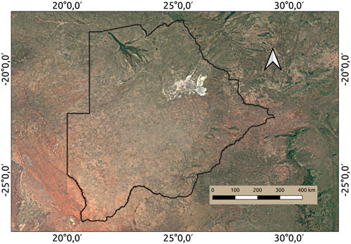
Figure 1. Study area map.

The study incorporates derived spectral indices, such as NDVI (Normalized Difference Vegetation Index), EVI (Enhanced Vegetation Index), and NDBI (Normalized Difference Built-Up Index), alongside a combination of field observations and carefully curated labels from the Dynamic World map. Due to the reported inaccuracies of the Dynamic World dataset in heterogeneous terrains (Xu et al., 2024), training polygons derived from Dynamic World were cross-checked against field survey data in areas where field measurements were available. To enhance the reliability of the ground truth data, visual cross-validation was performed using Google Earth imagery at additional training and validation locations where field surveys were not available. This hybrid approach for selecting training site polygons permits the generation of numerous reliable ground truth sampling points. These points are essential for training and testing the Transformer model, ultimately enabling the production of high-resolution, high-accuracy LULC maps tailored to Botswana’s ecologically diverse landscapes.

2.2 Data acquisition

Training data for LULC classification were sampled from the Dynamic World (DW) dataset, which provides near-real-time global land cover at 10 m spatial resolution using Sentinel-2 imagery and a deep learning framework (Brown et al., 2024). To ensure consistency with Landsat-derived features, training points were obtained from January–March 2022 from Landsat 8 OLI Collection 2 Level-2 imagery. This period was selected to capture optimal vegetation contrast during the peak growing season in Botswana (Zhang et al., 2003; Chen et al., 2019). Elevation data were derived from the Shuttle Radar Topography Mission (SRTM) Digital Elevation Model (DEM) at 30 m spatial resolution. All spatial datasets, including Landsat 8 OLI at 30 m resolution, Dynamic World at 10 m resolution, and SRTM DEM at 30 m resolution, were accessed through the Google Earth Engine (GEE) platform at: (https://developers.google.com/earth-engine/datasets/catalog). Nine DW-based LULC classes were used, with the “Snow and Ice” class replaced by “Pans” to capture Botswana’s salt flats, such as Makgadikgadi (Ringrose and Binns, 1996).

Stratified random sampling was applied to the DW map to select pixels representing all land cover classes for training and testing (Foody, 2002; Olofsson et al., 2021). Given the limited coverage of some classes in Botswana, the sampled DW points were cross-checked against independent field survey data and GE imagery. Only points where there was agreement among all three sources (DW, field surveys, GE) were retained. In cases where field data were not available, the points were included for training only if there was clear agreement between DW and GE. Importantly, if the DW classification disagreed with field survey observations, the point was relabeled according to the field survey, effectively refining the DW map. This procedure ensured that DW served as a reliable source of ground truth, while field surveys and GE provided independent verification of training/validation points, as shown in Table 1. Figure 2 shows the location of polygons used for training. Although Table 1 lists numerous polygons, the map displays them as small point clusters because several polygons are situated very close to each other, causing the enclosed pixels to appear stacked in the visualization at the current scale of the map.

Table 1

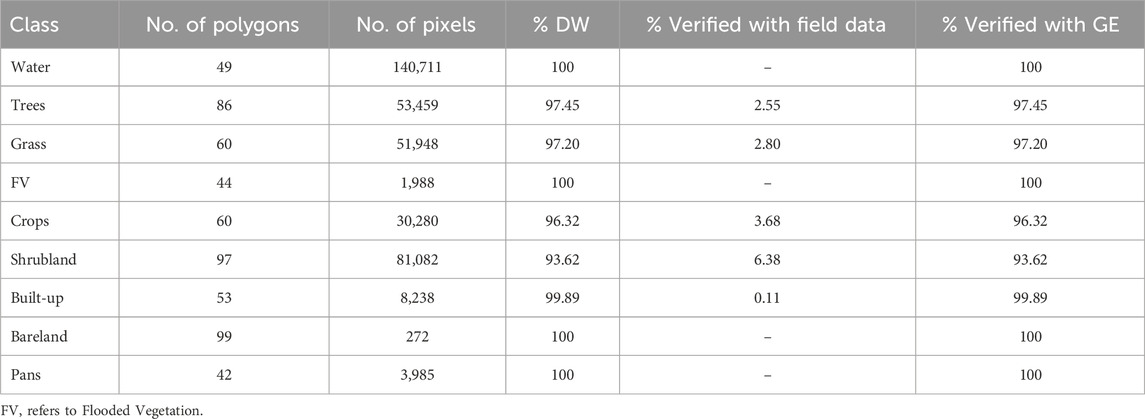
Table 1. Training/validation sampling summary.

Figure 2

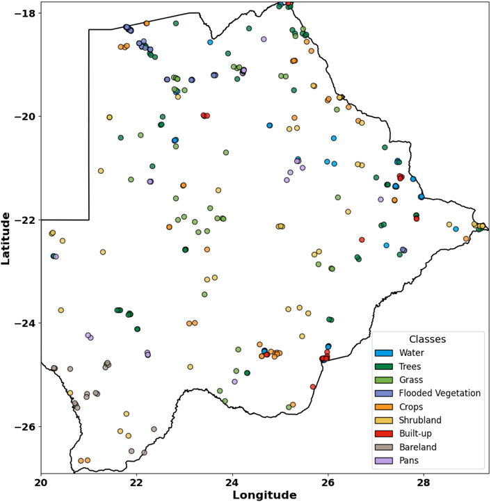
Figure 2. Location of polygons used for sampling.

From each pixel, spectral values were extracted from seven Landsat bands (SR_B1–SR_B7), which are well-suited for land surface classification (Roy et al., 2013; Zhu and Woodcock, 2012). In this study, Landsat 8 Collection 2 Level-2 Surface Reflectance (SR) imagery (“LANDSAT/LC08/C02/T1_L2”) was used. To ensure high-quality observations, a cloud and shadow masking procedure was applied using the quality flag labeled as QA_PIXEL band. Pixels affected by dilated clouds, cirrus, general clouds, and shadows were excluded by checking the corresponding QA bits. For each time period, the filtered images were composited using the median function to generate a single representative image for the study area. This approach ensures that only reliable, cloud-free pixels contribute to the analysis, supporting reproducibility of the results.

Spectral indices computed include the Enhanced Vegetation Index (EVI), which improves vegetation detection in high biomass regions (Huete et al., 2002); Normalized Burn Ratio (NBR) to detect burned areas and post-fire recovery (Key and Paine, 2006); Normalized Difference Moisture Index (NDMI) which indicates vegetation water content (Gao, 1996); Normalized Difference Water Index (NDWI), to emphasize water bodies (McFeeters, 1996); Normalized Difference Built-up Index (NDBI) to highlight built-up areas (Zha et al., 2003); Normalized Difference Bare soil Index (NDBaI)to improve detection of bare soil in arid zones (Chen et al., 2014). Elevation data from a digital elevation model (DEM) were also included to account for topographic variations that affect reflectance and microclimate Balthazar et al. (2012). The integration of the per-pixel spectral bands and indices and topographic in the per-pixel feature vector ensures robust classification of Botswana’s diverse landscape.

2.3 Model architecture

This study employs a Transformer model, a deep learning (DL) model, for multi-class LULC classification using 14 input features (i.e., constitute per-pixel feature vector): seven Landsat 8 OLI reflectance bands (SR_B1–SR_B7), six spectral indices (Table 2), and elevation data. The combination of raw spectral bands and indices enhances class separability by capturing diverse physical and biochemical surface characteristics (Zhu and Woodcock, 2012), while elevation data accounts for topographic effects on reflectance and land cover differentiation (Balthazar et al., 2012).

Table 2

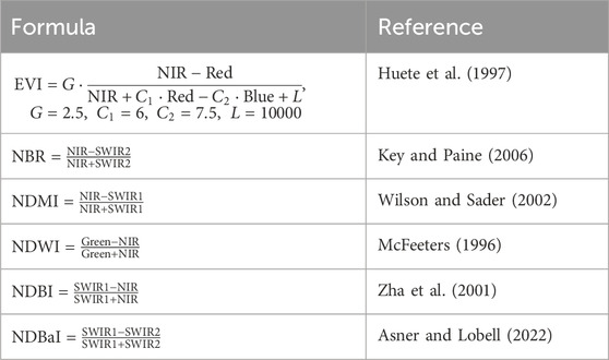
Table 2. Vegetation index formulas and references.

The input data were structured as tensors of shape (batch size, 14, 1), treating the 14 features as a sequence of tokens (Figure 3). Each feature was projected into a 64-dimensional embedding space using a dense layer, enabling richer feature representation, similar to applications in non-textual domains. Since the features do not possess an inherent sequential order, no positional encoding was applied. The features were used in the following fixed order to ensure: SR_B1, SR_B2, SR_B3, SR_B4, SR_B5, SR_B6, SR_B7, EVI, NBR, NDMI, NDWI, NDBI, NDBaI, and elevation. The embedded features passed through a Transformer Encoder block, consisting of: 1. Multi-Head Self-Attention (MHSA) with 4 attention heads, enabling the model to learn complex dependencies across features; 2. Position-wise Feed-Forward Network (FFN) with 128 hidden units, followed by a projection back to 64 dimensions, allowing the model to learn non-linear combinations of features; and 3. Residual connections, Layer Normalization, and Dropout (rate = 0.2) for improved training stability, convergence, and overfitting prevention. The output from the Transformer encoder was passed through a Global Average Pooling (GAP) layer, aggregating the feature sequence into a fixed-length vector. GAP reduces trainable parameters compared to flattening, aiding in preventing overfitting (Lin et al., 2003). Two fully connected layers with dropout regularization (rate = 0.3) were then applied to introduce non-linearities and improve generalization. The final classification was performed using a dense softmax output layer with 9 units, corresponding to the nine LULC classes (see Figure 3). The model was compiled using the Adam optimizer (Kingma and Ba, 2014) with a learning rate of $1\times 10^{-4}$, and categorical cross-entropy loss was used as the training objective. Classification accuracy was used as the primary evaluation metric. Adam was chosen for its adaptive learning rate and efficiency in training deep models, particularly in geospatial classification tasks (Zhu et al., 2023). This architecture effectively utilizes Transformer encoders to model feature interactions across the spectral bands and indices and topographic domains, enhancing LULC classification in diverse landscapes.

Figure 3

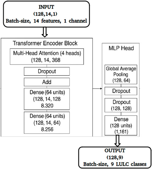
Figure 3. The Transformer model architecture used in the LULC classification.

2.4 Model training

During data collection from multiple polygons, the dataset was partitioned using a pre-assigned sample column, where each observation was tagged as either train or test. This column was generated through a stratified random sampling procedure, ensuring that 80% of the pixels from each land cover class were allocated to the training set and 20% to the testing set. This approach preserved class proportions across subsets and reduced bias from imbalanced class representation. The partitioning scheme was stored within the dataset to guarantee reproducibility. In total, 371,065 pixels were collected, with 296,852 pixels assigned to training and 74,213 to testing. Training proceeded iteratively, where the Transformer architecture learned to map input feature sequences to LULC labels by minimizing classification error. During each epoch, the model processed mini-batches, computed predicted probabilities, and compared them to true labels using categorical cross-entropy loss. Loss gradients were propagated backward to update model parameters via the Adam optimizer (Kingma and Ba, 2014), which is known for adaptive learning rates and stability in DL. The methodological flowchart is shown in (Figure 4).

Figure 4

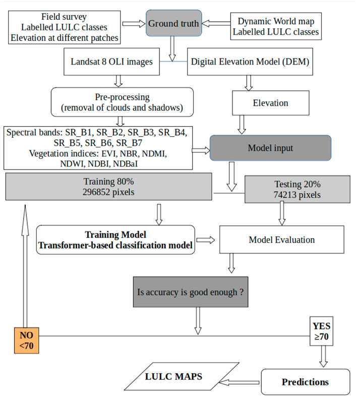
Figure 4. The methodology flow chart for LULC classification for Botswana.

To prevent overfitting and improve generalization, two regularization strategies were employed: dropout (set at 0.2 in the Transformer encoder and 0.3 in the fully connected layers) and early stopping. Dropout reduces co-adaptation of neurons, promoting a more robust representation (Hinton et al., 2012), while early stopping halted training when validation performance showed no improvement over a fixed number of epochs, preventing unnecessary training and overfitting. This training pipeline ensured the model effectively captured spectral-index interactions patterns while maintaining generalization. The design choices in training strategy, data partitioning, and regularization follow best practices for DL in remote sensing and LULC applications (Zhu et al., 2023).

2.5 Model evaluation

2.5.1 Standard evaluation metrics

The Transformer-based LULC classification model was evaluated using a range of standard evaluation metrics, including Overall Accuracy (OA), Producer’s Accuracy (PA), User’s Accuracy (UA), Precision, Recall, and F1 Score, as defined in Equations 1–6 based on the test dataset. These metrics provide various perspectives on classification quality and are widely used in remote sensing and land cover studies for accuracy assessment (Congalton, 1991; Stehman, 1997). The metrics capture overall model performance as well as class-wise performance, ensuring comprehensive evaluation, which is critical for applications like LULC mapping, where accurate delineation of land cover is essential. Overall Accuracy (OA) measures the proportion of correctly classified samples relative to the total number of test instances. It is defined as

$\text{OA}=\frac{\text{Number\hspace{0.17em}of\hspace{0.17em}Correctly\hspace{0.17em}Classified\hspace{0.17em}Pixels}}{\text{Total\hspace{0.17em}Number\hspace{0.17em}of\hspace{0.17em}Pixels}}\times 100(1)$

Producer’s Accuracy (PA) indicates the probability that a reference class is correctly identified, measuring omission error. It is defined as

$\text{PA}=\frac{\text{True\hspace{0.17em}Positives}}{\text{Total\hspace{0.17em}Reference\hspace{0.17em}Positives}}\times 100(2)$

User’s Accuracy (UA) measures the probability that a predicted class label corresponds to the true land cover. It is expressed as

$\text{UA}=\frac{\text{True\hspace{0.17em}Positives}}{\text{Total\hspace{0.17em}Classified\hspace{0.17em}Positives}}\times 100(3)$

Recall quantifies the proportion of actual positives correctly identified and is given by

$\text{Recall}=\frac{\text{True\hspace{0.17em}Positives}}{\text{True\hspace{0.17em}Positives}+\text{False\hspace{0.17em}Negatives}}(4)$

Precision measures the proportion of true positives among all samples classified as a given class, and is calculated as

$\text{Precision}=\frac{\text{True\hspace{0.17em}Positives}}{\text{True\hspace{0.17em}Positives}+\text{False\hspace{0.17em}Positives}}(5)$

F1 Score is the harmonic mean of Precision and Recall, providing a balanced measure that accounts for both false positives and false negatives. It is computed as

$\text{F}1=2\times \frac{\text{Precision}\times \text{Recall}}{\text{Precision}+\text{Recall}}(6)$

2.5.2 Disagreement measures in thematic accuracy assessment

In recent years, the use of the Kappa coefficient in thematic accuracy assessment has been increasingly criticized and discouraged in the remote sensing literature. Several studies have argued that Kappa can be misleading and does not provide a clear diagnostic of classification errors (Foody, 2020; Olofsson et al., 2011). As an alternative, the use of disagreement measures—namely, Total Disagreement (TD), Quantity Disagreement (QD), and Allocation Disagreement (AD)—has been recommended for evaluating the accuracy of land use and land cover (LULC) classifications (Foody, 2020; Olofsson et al., 2011) as shown in Equations 7–9.

Total Disagreement represents the proportion of incorrectly classified samples and is simply defined as:

$\text{TD}=1-\text{OA},(7)$

where $\text{OA}$ is the overall accuracy of the classification. Quantity Disagreement quantifies the disagreement due to differences in the amount (quantity) of each class between the reference and the classified maps. It is computed as:

$\text{QD}=\frac{1}{2N}{\displaystyle \sum _{k=1}^n}\left|R_k-P_k\right|,(8)$

where $R_k$ and $P_k$ are the total number of reference and predicted pixels, respectively, for class $k$, $n$ is the number of classes, and $N$ is the total number of samples. Allocation Disagreement reflects the disagreement that arises when the quantities are correct but the spectral-index interactions allocation of class labels is incorrect. It is given by:

$\text{AD}=\text{TD}-\text{QD}.(9)$

Together, QD and AD provide a more interpretable and diagnostic decomposition of classification error, making them particularly suitable for assessing the quality of thematic maps.

2.5.3 Model consistency beyond training period

Further evaluation of the trained model is carried out using input data beyond the training period of January-March 2022. Predictions for 2014, 2019, and 2024 were generated using the same data sources and the January–March time frame applied in 2022 for model training and testing. The landcover dynamics over a period of 10 years is assessed in terms of consistency with seasonal and interannual variability as well as the evolving LULC dynamics.

3 Results and discussions

3.1 Model training

The Transformer-based classification model achieved strong performance during training, with an OA of 95%. These metrics indicate a high level of consistency between predicted and reference labels, exceeding chance expectations despite slight class imbalances. This is consistent with prior research showing the Transformer’s capacity to capture complex spatial and contextual features in remote sensing data (Han et al., 2022; Guo et al., 2024).

The model was trained on 296,852 labeled pixels across nine LULC classes and performed well in most categories. The overall producer’s accuracy (PA) varied among the nine land cover classes, reflecting differences in per-pixel feature vector distinctiveness and classification performance (see Table 3). The accuracy rates were as follows: Water (99.91%), Trees (96.73%), Shrubland (95.79%), and Bareland (95.89%). Additionally, the accuracy for Grass was 88.72%, Crops 87.52%, Built-up areas 82.69%, and Flooded Vegetation 80.41%. The results indicate excellent model performance, likely due to its unique and easily identifiable spectral signature, aided by the use of vegetation indices that enhanced separability (Zhang et al., 2020; Zhao et al., 2020). However, the Pans class showed lower PA (56.82%), likely due to seasonally varying signatures contained in the spectral bands and indices, which were affected by contamination from elevated water levels in some summers. Additionally, its low frequency in the training set made it harder to distinguish from water bodies during the wet season (Chiloane et al., 2020). The Flooded Vegetation and Built-up classes also displayed moderate PA values (0.79), suggesting challenges in differentiating them due to spectral mixing in heterogeneous zones, a common issue noted in Transformer-based models (Marjani et al., 2025). Despite these challenges, the model demonstrated high UA $(>0.90)$ for all classes except for Flooded Vegetation, which achieved 83.15%. Although Pans have a PA of (56.82%), it achieved a high UA (0.97), indicating that when it did classify a pixel as Pan, it was usually correct. This behavior reflects a conservative learning approach prioritizing precision over recall, common in deep models when trained on imbalanced data (Johnson and Khoshgoftaar, 2019). Overall, the training results demonstrate that the Transformer model successfully learned complex LULC patterns, leveraging distinct information contained in per-pixel feature vector, and effectively demonstrated class-specific learning (Voelsen et al., 2016).

Table 3

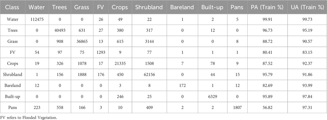
Table 3. Confusion Matrix with Producer’s and User’s Accuracy for Botswana based on the training dataset.

3.2 Model evaluation

The Transformer-based land cover classification model was evaluated using a held-out testing dataset comprising 74,213 pixels. The model achieved an overall accuracy (OA) of 95.31%, corresponding to a total disagreement (TD) of 4.69%. Decomposition of the disagreement revealed a quantity disagreement (QD) of 1.25% and an allocation disagreement (AD) of 3.44%. These results indicate that most of the classification error arises from the per-pixel feature vector allocation mismatches, mainly due to mixed signatures from mixed vegetation cover within the pixel rather than systematic quantity errors, suggesting that the model effectively captures class proportions but encounters minor spatial misplacements. Such low levels of QD and AD underscore the model’s strong generalization capability and spatial consistency, even in ecologically complex and heterogeneous dryland environments. These findings reinforce the suitability of Transformer-based architectures for land use and land cover (LULC) classification, particularly due to their ability to model long-range dependencies and contextual information within high-dimensional satellite imagery. (Han et al., 2022; Guo et al., 2024; Marjani et al., 2025).

Moreover, the LULC created from the Landsat 8 image was assessed against both True Color Composite (TCC) and False Color Composite (FCC). TCC, created using Bands 4 (Red), 3 (Green), and 2 (Blue), offers a straightforward visualization of land cover. In this composite, healthy vegetation appears darker due to its strong absorption in the red and blue wavelengths, while a brownish color represents unhealthy or sparse vegetation. Bare surfaces, such as deserts or urban areas, are distinguishable by their whitish appearance, reflecting high amounts of visible light. However, due to limitations in spectral differentiation, certain land cover types with similar reflectance values in the visible spectrum may be challenging to distinguish. This issue is particularly evident when distinguishing between areas with similar vegetative cover or bare soils (Song et al., 2017).

To overcome these challenges and enhance the discrimination of LULC types, a false color composite (FCC) was generated using Bands 7 (Shortwave Infrared), 5 (Near-Infrared), and 3 (Green). The FCC allows for a more effective differentiation of vegetation and other land cover types, as healthy vegetation appears in shades of green due to strong reflection in the near-infrared (NIR) band. This makes it easier to identify dense vegetation areas (Song et al., 2017). Areas exhibiting reddish tones in the FCC are typically indicative of stressed or sparse vegetation, which may also reflect transitional zones where vegetation is either degrading or upgrading. Such patterns are often associated with varying soil moisture levels that influence vegetation growth (Li et al., 2011). For instance, in the Okavango Delta (Figure 5), areas with saturated soils, shadowed wetlands, or waterlogged vegetation appear as dark regions in the TCC (Figure 5a) and green in the FCC images (Figure 5b), whereas same areas appear as trees and grass in the predicted map (Figure 5c). In contrast, they appear as trees, grass, and shrubland in the Dynamic World map (Figure 5d), reflecting the specific environmental conditions of wetlands and floodplains (Fang et al., 2010).

Figure 5

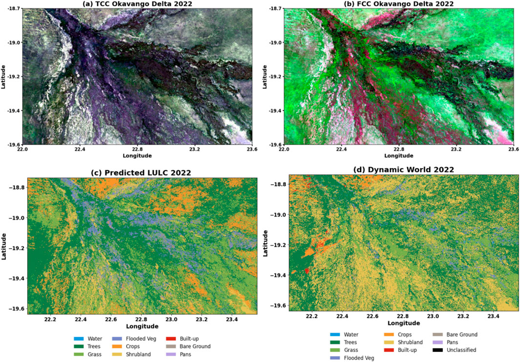
Figure 5. TCC (a) and FCC (b) alongside the model prediction (c) and Dynamic World image (d) from January to March 2022 around Okavango Delta.

The model’s performance was evaluated using PA and UA metrics derived from the testing dataset. These values are summarized in Table 4, where the Pans class recorded the lowest PA of 47.77%., indicating significant omission errors and difficulty in identifying all instances of this ephemeral and seasonally dynamic land cover type. However, the UA for Pans was 99.54%, suggesting that while the model rarely predicted pixels as Pans, those predictions were highly accurate. This conservative prediction behavior, favoring high precision over recall, is common for underrepresented or ambiguous classes in classification tasks and has been reported in similar studies dealing with small-scale or transient landscape features (Graves et al., 2016). Flooded Vegetation showed a PA of 83.78% and a UA of 52.32%. This indicates that while most actual Flooded Vegetation pixels were successfully identified (high PA), the model also misclassified a substantial proportion of other classes as Flooded Vegetation, resulting in a lower UA, likely due to misclassifications often occurring at boundaries between water and vegetated areas (Feng et al., 2015). This is also evident from the predicted map (Figure 5c) than in the Dynamic World map (Figure 5d), which indicates mostly trees closer to Flooded Vegetation.

Table 4

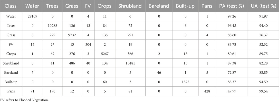
Table 4. Confusion Matrix with Producer’s and User’s Accuracy for Botswana based on testing dataset.

Water bodies, which exhibit low reflectance in both the NIR and SWIR bands, appear blue in the FCC image (Figure 6a) and light green and grey in TCC (Figure 6b), consistent with findings from previous studies (Ma et al., 2019). Class-specific accuracy metrics provide further insights into the model’s performance, as summarized in (Table 4). The water class exhibited the highest PA of 97.26% and a UA of 91.97%, reflecting the model’s excellent capability to detect and correctly classify water bodies. This is consistent with the well-documented spectral distinctiveness of water, which generally shows strong absorption in the near-infrared and shortwave infrared regions (Sagan et al., 2020; Ma et al., 2019). Therefore, the predicted map is better at capturing the observed vegetation condition in the Okavango Delta than the Dynamic World map. In contrast, the predicted map (Figure 6c) shows water and Pans, whereas the Dynamic World map (Figure 6d) shows water and bareland. This indicates that the Transformer model misclassifies the Pan as water due to spectral similarity and the presence of a wet Pan surface during the January to March period, due to seasonal rainfall. On the other hand, the Dynamic World map does not recognize Pan in its classification, and all water-free Pan areas are mostly labeled as bareland (Figure 6d).

Figure 6

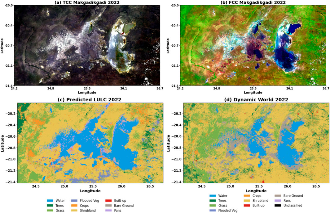
Figure 6. TCC (a) and FCC (b) alongside the model prediction (c) and Dynamic World image (d) from January to March 2022 around Makgadikgadi Pans.

Trees were similarly well predicted, with a PA of 0.96 and UA of 0.94, demonstrating the model’s strong ability to capture the unique spectral and structural features associated with forested areas. These findings are supported by previous studies that show Transformer models effectively distinguish vegetative classes when provided with multispectral and index-rich input data (Reedha et al., 2022). The attention mechanisms within Transformer architectures allow for better modeling of tree canopy textures as the reflectance signatures in the per-pixel feature vector are highly influenced by the canopy texture. Grass and Shrubland were also predicted with relatively high PA values (0.85 and 0.87, respectively), indicating that the model successfully captured the spectral characteristics representative of these vegetation types. However, the UA for Grass (0.76) suggests some degree of confusion, likely due to its spectral similarity with other green vegetation, particularly Crops. Shrubland had a higher UA of 0.82, implying better reliability in the predictions. This reflects the Transformer’s ability to utilize broader and distinct signals from each per-pixel feature vector, yet also highlights persistent challenges in distinguishing between vegetation types with overlapping reflectance patterns (Zhao et al., 2023). The Chobe area in Botswana has a lot of Trees, Shrubland, and Grass, especially during the rainy season. The model was able to clearly show these land cover types, matching well with what is seen in the TCC and FCC images (Figures 7a,b), consistent with relatively higher PA and UA for the vegetation classes (Table 4). Compared to the Dynamic World map, the model performed better because it picked up small differences in vegetation and more closely followed the natural patterns of the area. The grass area bounded by shrubland in pink color in FCC (Figure 7a) and violet in TCC (Figure 7b) formed a natural landscape pattern. This pattern, including tree vegetation on the exterior side of the shrubland, is well captured by the map produced by the Transformer model (Figure 7c). In contrast, the DW map fails to capture the distinct natural shrubland boundary between grass and trees (Figure 7d).

Figure 7

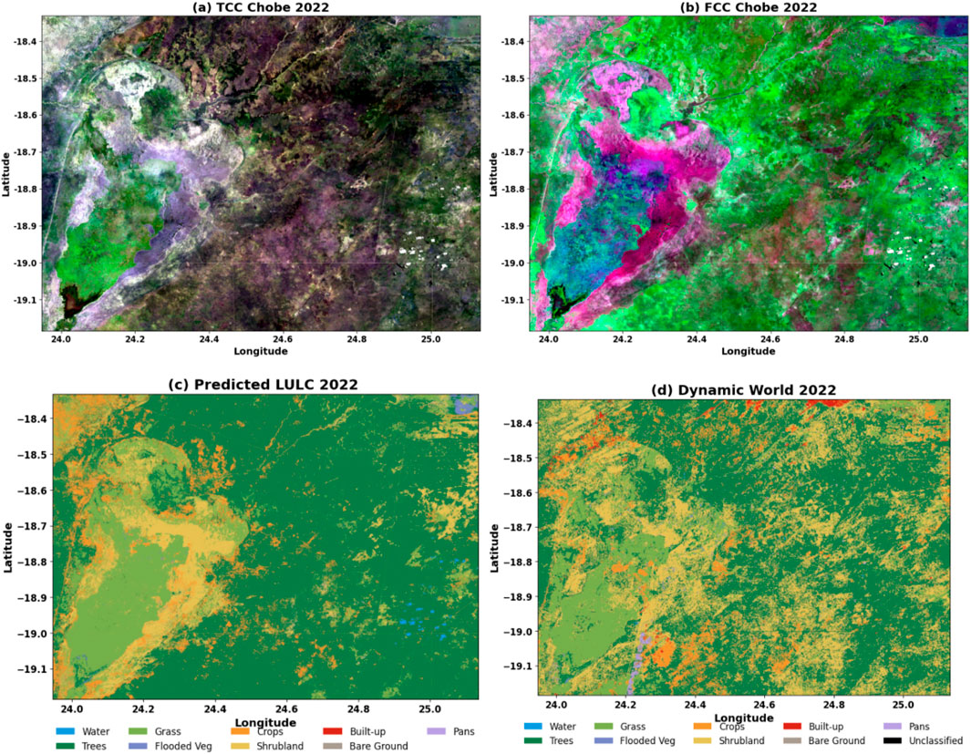
Figure 7. TCC (a) and FCC (b) alongside the model prediction (c) and Dynamic World image (d) from January to March 2022 in Chobe District.

Bareland achieved a moderate PA of 72.87% and a high UA of 88.85%. This indicates that while the model missed some Bareland instances, its predictions were largely accurate when it did assign pixels to this class. The spectral distinctiveness of bare soil, particularly in the visible and SWIR bands, supports the model’s high reliability for this class, consistent with prior findings in arid and semi-arid regions (Milewski et al., 2022). In Botswana, barren areas are mainly located in the Kgalagadi District, as shown in Figure 8. Visually, the Predicted LULC image (Figure 8c) closely follows the whitish pattern seen in the TCC (Figure 8a) and pink landscape in the south and western gradient of the FCC image (Figure 8b), where bareland areas are clearly identified. In contrast, the Dynamic World map (Figure 8d) shows dominantly shrubland over the same areas.

Figure 8

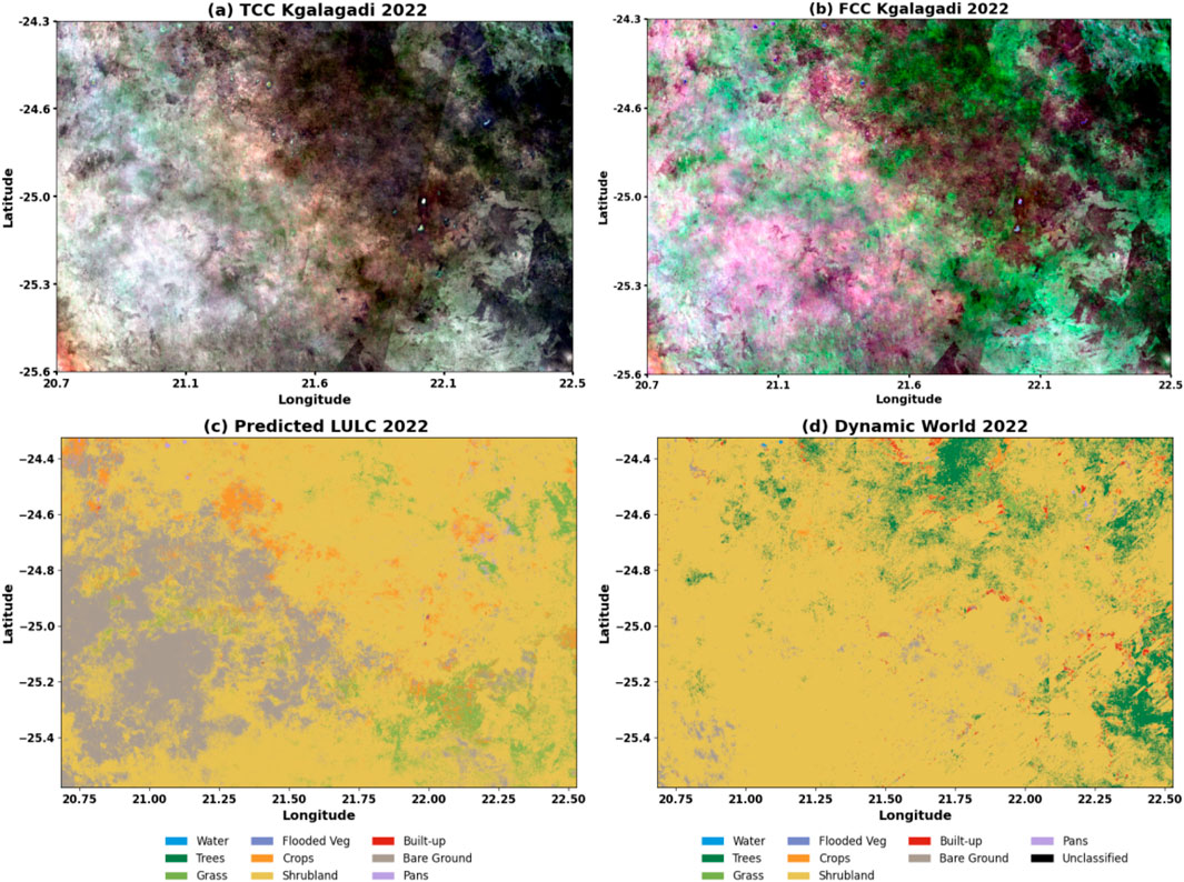
Figure 8. TCC (a) and FCC (b) alongside the model prediction (c) and Dynamic World image (d) from January to March 2022 in Kgalagadi District.

For the Built-up class, the model achieved a PA of 85.37%, meaning most actual built-up areas were correctly identified. The UA was 94.59%, showing that the majority of predicted built-up pixels were accurate. The high PA highlights the model’s strong ability to capture built-up areas, while the high UA suggests that when the model predicts built-up areas, it is mostly reliable. The strong performance can be attributed to the clear spectral patterns of built-up surfaces, such as rooftops and roads, which are easily identifiable in both the TCC and FCC images (Figures 9a,b). The Predicted LULC map captured built-up areas in Gaborone City more accurately (Figure 9c) than the Dynamic World map (Figure 9d). The Dynamic World does not distinguish between building blocks and bare land, dense settlement and sparse settlement, and roads from other structures within the city, highlighting the limitations of GLC maps in capturing fine-scale urban features in the local context. In urban regions like Gaborone, the predicted map (Figure 9c) successfully resolves urban morphology, roads, vegetation, buildings, and water bodies visible in the TCC and FCC composites (Figures 9a,b). In comparison, the Dynamic World map (Figure 9d) shows a homogeneous block of built-up land, failing to distinguish intra-urban land cover heterogeneity. Although Dynamic World is derived from Sentinel-2 imagery with a nominal 10 m spatial resolution, this discrepancy suggests local-level generalization or smoothing in the global product, which undermines the expected benefits of higher resolution. This paradox highlights the importance of high-quality, context-specific training data, as emphasized by Xu et al. (2021).

Figure 9

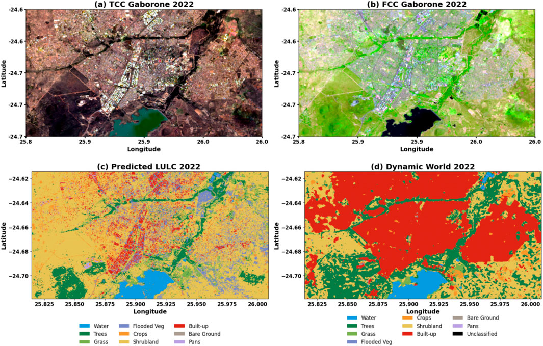
Figure 9. TCC (a) and FCC (b) alongside the model prediction (c) and Dynamic World image (d) from January to March 2022 in Gaborone City.

Overall, the model’s testing performance reinforces the efficacy of Transformer-based approaches for LULC classification, particularly when dealing with complex landscapes. The attention mechanism enables the model to focus on relevant per-pixel feature vector across the input image, thereby contributing to improved generalization and class discrimination. These findings align with the emerging literature, which highlights Transformers as a state-of-the-art alternative to CNNs and traditional machine learning algorithms in remote sensing classification tasks (Adegun et al., 2023; Zhao et al., 2023).

Flooded Vegetation and Pans were among the most challenging classes to classify accurately. Table 5 presents a side-by-side comparison of PA and UA for these classes based on both the training and testing datasets. For Flooded Vegetation, the model achieved relatively high PA (80.41% on training and (83.78%) on testing, indicating that most actual Flooded Vegetation pixels were correctly identified. However, the UA was considerably lower on the testing dataset (52.32%), suggesting that a substantial portion of pixels predicted as Flooded Vegetation actually belonged to other classes. This discrepancy likely stems from spectral similarities between Flooded Vegetation and nearby vegetated areas, such as Trees or Grass, which can confuse the classifier.

Table 5

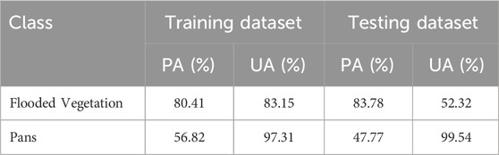
Table 5. PA and UA for Flooded Vegetation and Pans based on training and testing datasets.

For Pans, the UA remained very high (97.31%) on training (99.54%) on testing, demonstrating that pixels predicted as Pans were almost always correct. In contrast, PA was relatively low, especially on the testing dataset (47.77%), indicating that the model failed to detect a significant fraction of actual Pans. This limitation is likely related to the seasonal timing of the imagery (January–March), when many pans may have been submerged under water, reducing their spectral distinctiveness and making them less detectable.

The performance of the Transformer-based model was further evaluated using several metrics, including precision, recall, and the F1 score, across various land cover classes, as shown in (Figure 10). These metrics provide a more nuanced understanding of the model’s ability to not only identify land cover types but also minimize both false positives and false negatives. Precision, recall, and F1 score are essential for assessing classification performance, particularly when dealing with imbalanced datasets and complex land cover types (Sim et al., 2024).

Figure 10

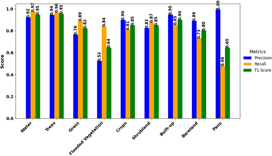
Figure 10. Precision, Recall and F1-Score of the Transformer model based on the testing dataset.

The Water class attained a high precision (0.92), meaning 92% of pixels predicted as water were correctly classified. This excellent result aligns with earlier research, which highlights the reliability of remote sensing techniques in identifying water bodies, owing to their unique spectral signatures—particularly in the visible and near-infrared wavelengths (Fu et al., 2022). The Water class achieved a recall of 0.97, indicating that the model accurately detected 97% of actual water pixels. This high recall demonstrates the model’s effectiveness in fully capturing the spatial distribution of water bodies, which is essential for reliable hydrological and environmental monitoring (Wang et al., 2021). An F1 score of 0.95, reflecting a perfect balance between precision and recall, underscores the model’s strong and consistent performance in accurately detecting water features.

The high precision, recall, and F1 score of 0.94, 0.96, and 0.95, respectively, suggest that the model is highly reliable in identifying the Tree class. This is supported by studies that have shown Transformer-based models excel in classifying vegetation types due to their ability to capture spatial context and complex spectral patterns (Ma et al., 2019). In particular, the use of spectral indices, such as NDVI, enhances the classification accuracy of vegetation (Navidan et al., 2021), which may explain the model’s strong performance in this class.

The Grass class achieved a precision of 0.76, indicating that 76% of the pixels predicted as Grass were correctly classified. Its recall reached 0.89, meaning that 89% of the actual Grass pixels were accurately identified by the model. The corresponding F1 score of 0.82 demonstrates a strong balance between precision and recall, highlighting the model’s reliable performance in detecting Grass. This level of accuracy suggests the model effectively distinguishes Grass from other vegetative land cover types, although some spectral overlap with other land cover types may still account for occasional misclassifications. Such performance is consistent with findings in prior studies, which note that vegetation classes like Grass can be well distinguished using multispectral remote sensing data, though confusion with spectrally similar vegetation types can occur (Foody, 2002; Thenkabail et al., 2011).

The Flooded Vegetation class demonstrated a precision of 0.52, meaning that 52% of the areas predicted as Flooded Vegetation were correctly classified. A recall of 0.84 indicates that the model successfully identified 84% of all actual Flooded Vegetation instances. The corresponding F1 score of 0.64 reflects a moderate balance between precision and recall, suggesting that the model detects Flooded Vegetation reasonably well but still struggles with misclassifications. The relatively low precision highlights that a notable proportion of other classes, particularly spectrally similar ones such as Water bodies or dense Tree cover, were incorrectly labeled as Flooded Vegetation. This challenge of class separability has also been noted by Feng et al. (2015), who reported that spectral overlap can complicate the accurate mapping of inundated vegetation using satellite imagery.

The Crops class achieved a precision of 0.90, meaning that 90% of the pixels predicted as Crops were accurately classified. This high precision indicates that the model was efficient at identifying Crops while minimizing false positives. The recall value of 0.81 indicates that the model correctly identified 81% of all actual Crop pixels. While this is a strong result, it suggests that the model did miss 19% of the actual Crop pixels, potentially due to spectral confusion with other types of vegetation or misclassification of crop fields with similarly vegetated areas. The F1 score of 0.85 indicates a balanced performance between precision and recall, confirming the model’s robustness in detecting Crops. This score suggests that, overall, the model performs well in classifying Crop areas, although some minor misclassification errors might occur due to spectral overlaps with other vegetation types, such as Grass or Flooded Vegetation. In remote sensing, crops often exhibit unique spectral signatures that can be effectively distinguished using satellite imagery, but challenges can arise due to seasonal variations, growth stages, and similarities to other land cover types (Jensen, 2005). The model’s high precision, however, suggests that it was particularly successful at distinguishing Crops from non-crop land cover types.

The Shrubland achieved a precision of 0.82, meaning that 82% of the pixels predicted as Shrubland were correctly identified. The recall value of 0.96 indicates that the model successfully detected 0.87% of all actual shrubland pixels, demonstrating strong sensitivity and the model’s ability to accurately capture the extent of Shrubland areas. The F1 score of 0.85 reflects a high-performing model, with both precision and recall values closely aligned. This high performance suggests that the model is quite effective at identifying shrubland. However, there may still be occasional confusion with other land cover types with similar spectral signatures, such as Grass or Tree classes, although this is not indicated to be a significant issue given the high recall and F1 score. Shrubland areas are typically characterized by distinct vegetation signatures, making them relatively easy to detect with high accuracy. However, challenges may arise in cases of heterogeneous landscapes where Shrubland coexists with other land cover types, or during periods of low vegetation activity (e.g., droughts) (Liu et al., 2017).

The Built-up class achieved a precision of 0.95, indicating that 95% of the pixels classified as Built-up were accurately identified. However, the recall for Built-up areas was 0.85, indicating that the model identified only 85% of all actual Built-up pixels. As a result, the F1 score was 0.90, reflecting a reasonable balance between precision and recall. These results suggest that while the model is effective in detecting Built-up areas, confusion with spectrally similar land cover types, likely bareland, may contribute to the lower recall. This issue of spectral overlap between Built-up areas and bare land has been documented in previous studies, where materials such as concrete and soil have similar reflectance characteristics, leading to misclassification (Zhou and Huang, 2020; Jin et al., 2013). The Bareland class achieved a high precision of 0.89, meaning that 89% of the pixels predicted as Bareland were correctly classified. The recall of 0.73 indicates that the model successfully captured 73% of all actual Bareland pixels, although some were missed. The resulting F1 score of 0.80 reflects a good balance between precision and recall, suggesting that the model performs effectively in distinguishing Bareland from other land cover types, with slightly better performance in avoiding false positives than in capturing all true instances. Studies have shown that bareland exhibits a low reflectance in the visible spectrum, making it easily distinguishable from vegetated or built-up areas (Zhou et al., 2018; Lu and Weng, 2011).

The model’s performance on the Pans class, which represents saline surface areas, achieved a perfect precision of 1.00, meaning that all pixels predicted as Pans were correctly classified. This highlights the model’s strong reliability in avoiding false positives for this class. However, the recall of 0.48 indicates that the model detected less than half of the actual saline areas, likely due to seasonal effects in the training data, as many pans may have been submerged during the rainy season. The resulting F1 score of 0.65 reflects a moderate overall performance, showing that while the model excels at precision, it substantially underestimates the full spatial extent of pans. This issue is consistent with findings from previous studies, which note that saline surfaces often exhibit spectral confusion with water bodies and bare soils, particularly under variable moisture conditions (Zhang et al., 2019; Zhao et al., 2018).

Overall, the assessment of the model during testing (Table 4) and visual inspection of areas dominated by specific classes (Figures 5–9) as well as precision, recall, and the F1 score demonstrated strong model performance across most land cover classes. The Transformer model exhibited strong overall performance, with F1-scores above 0.84 for all classes except Flooded Vegetation and Pans, which achieved 0.64 and 0.65, respectively. Although the model performed satisfactorily on Flooded Vegetation and Pans, misclassifications with spectrally similar classes lowered the precision for Flooded Vegetation (0.52), while the recall for Pans was reduced (0.48), likely because many Pans were submerged under water during the rainy season (January–March). Despite these challenges, the model proved effective in capturing key land cover types, demonstrating its suitability for large-scale environmental monitoring and land-use assessment. The Transformer-based model’s performance aligns with previous studies that highlight the strength of attention mechanisms in handling complex and heterogeneous land cover types (Guo et al., 2024).

3.3 Assessment of the prediction of the transformer model beyond training periods

The trained Transformer model was applied to predict LULC during the January–March period for the years 2014, 2019, and 2024, utilizing the same 14 per-pixel feature vector consisting of spectral bands, spectral indices, and elevation, as the input vector used during training. To qualitatively assess prediction accuracy, we visually compared the model outputs against True Color Composite (TCC) and False Color Composite (FCC) images, and against the Dynamic World map, which we use as a baseline GLC. For both 2014 and 2019, the predicted LULC maps demonstrate strong visual congruence with FCC and TCC composites (Figures 11, 12). In 2019, the model (Figure 12c) captures more detailed land cover transitions than the Dynamic World map (Figure 12d), which tends to generalize land cover into homogeneous patches. This supports the findings of Xu et al. (2024), who observed that Dynamic World maps tend to smooth spatial transitions in heterogeneous landscapes, resulting in reduced thematic granularity. Liu X. et al (2021) similarly noted that globally optimized models often fail to capture local-scale complexity, especially in ecosystems with high spatial heterogeneity such as agro-pastoral zones or riparian corridors. However, the absence of Dynamic World data for 2014 limits historical assessments. This lack of temporal depth has been flagged by Brown et al. (2024) as a significant constraint when conducting long-term land cover change analyses. In contrast, the current Transformer model demonstrates flexibility by leveraging historical satellite imagery to generate retrospective LULC predictions, supporting more robust temporal assessments.

Figure 11

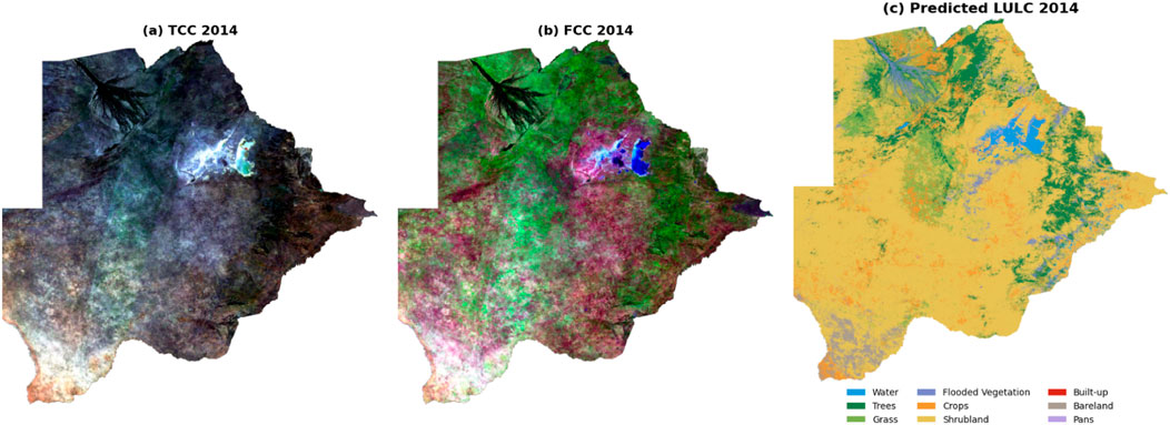
Figure 11. TCC (a) and FCC (b) alongside the model prediction (c) from January to March 2022.

Figure 12

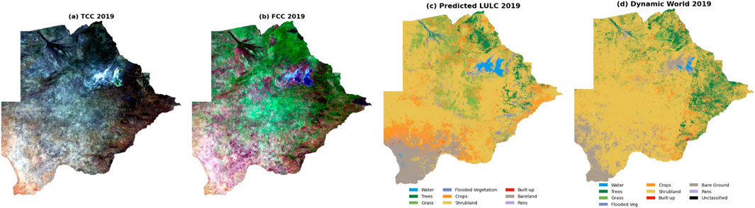
Figure 12. TCC (a) and FCC (b) alongside the model prediction (c) and Dynamic World image (d) from January to March 2019.

Several distinct land cover patterns during January-March 2024 emerge from the composites and predicted LULC maps, offering critical insights into model performance (Figure 13). Wetlands and water-saturated vegetated areas, such as those in the Okavango Delta, manifest in darker shades, and water bodies—especially near the Makgadikgadi Pans—are highlighted in blue in the FCC images. This spectral behavior is consistent with findings by Braga et al. (2021), who emphasize the role of NIR and SWIR in vegetation and moisture differentiation. Similarly, Kirimi et al. (2018) reported that FCC imagery is particularly effective in delineating seasonal water bodies in sub-Saharan Africa. The 2024 predicted LULC map (Figure 13c) shows strong visual alignment with both the FCC (Figure 13a) and TCC (Figure 13b) images, with clearer land cover class boundaries compared to the Dynamic World map (Figure 13d). The Dynamic World map significantly underrepresents water features over the Pans region, contrary to the FCC and predicted maps that more accurately capture the expected inundation during the summer rainy season. This mismatch may stem from the Dynamic World algorithm’s reduced sensitivity to ephemeral or shallow water bodies, a limitation noted in global classifiers that rely on coarser temporal and spatial generalizations (Sogno et al., 2022).

Figure 13

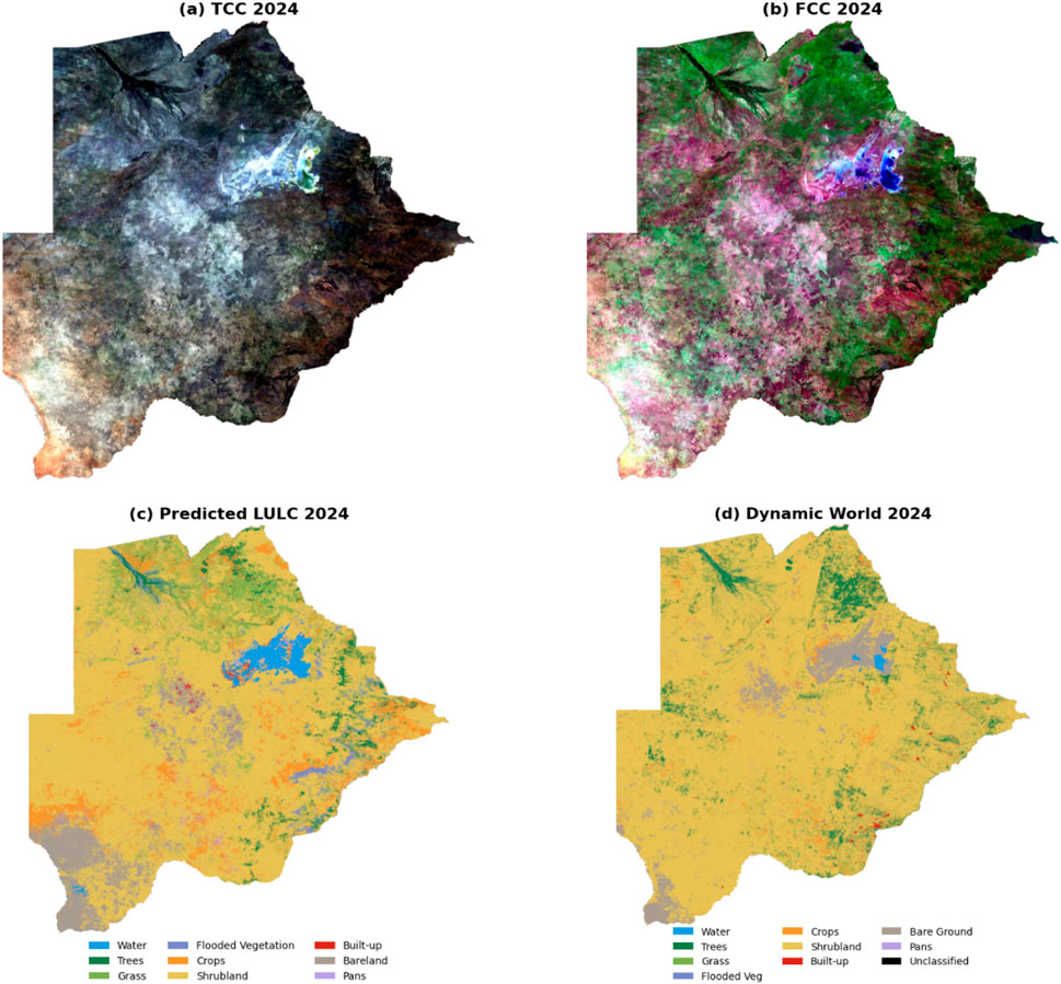
Figure 13. TCC (a) and FCC (b) alongside the model prediction (c) and Dynamic World image (d) from January to March 2024.

Reddish patches in the FCC, indicating vegetation under stress or sparsity, correspond to several predicted vegetation classes. Dense green zones align with healthier vegetation types, again underscoring the model’s nuanced classification capacity in complex ecosystems. This observation aligns with the challenges discussed by Liu et al. (2007), who highlight spectral similarity among vegetation types as a persistent hurdle in multispectral classification. Moreover, Bareland classes demonstrate a high degree of consistency across FCC, TCC, and the predicted map, in contrast to the Dynamic World map, which appears spatially inconsistent. Notably, built-up areas adjacent to Bareland sometimes exhibit spectral confusion, especially in arid zones where soil and construction materials share reflectance properties (As-Syakur et al., 2012).

In summary, although the Dynamic World map offers valuable insights at a global scale, its generalized classification strategy and localized resolution limitations constrain its application in complex, heterogeneous environments. By contrast, the Transformer-based model, trained on context-specific data and enhanced pixel level signature, provides more accurate, detailed LULC classifications. These findings underscore the importance of localized training data and high-resolution imagery for producing reliable LULC maps, echoing recommendations from recent literature (Phinzi et al., 2023). The enhanced interpretability and spatial resolution of the predicted maps affirm their utility in supporting environmental monitoring, land management, and adaptation planning in data-sparse regions.

3.4 The impact of misclassification on the fidelity of LULC change estimates in the recent decade

The dynamics of LULC in Botswana were assessed using a Transformer model and the Dynamic World (DW) land cover product. The Transformer model outputs detailed LULC statistics for 2014, 2019, and 2024 (Table 6) at 30 m resolution, while the DW product offers corresponding estimates for 2019 and 2024 (Table 7) at 10 m resolution. A comparative analysis reveals notable inconsistencies between the two, particularly for vegetation, agricultural, and hydrological classes. These discrepancies underscore the limitations of the DW product in accurately capturing transitional and heterogeneous land cover, especially in dryland environments.

Table 6

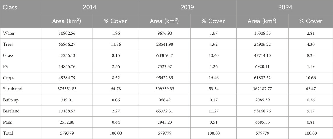
Table 6. Land Cover Statistics for 2014, 2019, and 2024 based on the Transformer model (30 resolution).

Table 7

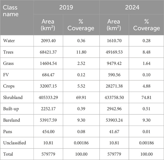
Table 7.  Land Cover Statistics Based on Dynamic World Map for 2019 and 2024 (10 m resolution).

Shrubland emerges as the dominant class in both datasets; however, DW exhibits an unrealistically high and steadily increasing shrubland extent—from 69.91% in 2019 to 74.81% in 2024. In contrast, the Transformer model reveals more plausible temporal variations: a decline from 64.78% in 2014 to 53.34% in 2019, followed by a rebound to 62.47% in 2024. The inflated shrubland coverage in DW likely results from misclassification of spectrally similar vegetation types such as grasslands and croplands, a known limitation in previous global assessments (Soubry and Guo, 2022). This is also evident when examining the color composites (Figures 7a,b) and the Transformer map (Figure 7c) of the Chobe district. The DW classification misidentifies trees as shrublands (Figure 7d) in areas outside of a narrow band of shrubland depicted in the color composites. This tendency toward overgeneralization reduces DW’s sensitivity to short-term ecological changes and anthropogenic land use pressures.

Cropland areas are markedly underestimated in the DW product, with coverage reported at only 5.52% in 2019 and 4.88% in 2024. In contrast, the Transformer model captures a more dynamic cropland trend; an increase from 8.52% in 2014 to 16.46% in 2019, followed by a decline to 10.66% in 2024, which likely reflects inter-annual variations in rainfall and planting patterns within the January–March peak growing season. The elevated crop area in 2019 may coincide with higher rainfall or intensified agricultural activity, while the subsequent reduction in 2024 could result from fallow periods due to a shortage of rainfall. These patterns are consistent with known seasonal land use changes, climatic variability, or temporary abandonment (Lark et al., 2020). The DW product’s limited ability to resolve such temporal variability reflects challenges in distinguishing spectrally overlapping classes within mixed agro-ecological systems.

Tree cover is overestimated in DW (11.80% in 2019), compared to 4.92% in the Transformer model, although estimates begin to converge by 2024. The Transformer model depicts a more credible pattern of forest decline—from 11.36% in 2014 to 4.30% in 2024, aligning with known deforestation pressures such as logging and agricultural encroachment (Hansen et al., 2013). The inflated and static tree estimates in DW likely stem from confusion with tall shrubland or regenerating vegetation, pointing to limitations in spectral separability and temporal smoothing within the DW classification pipeline. Sensor differences in both crop and tree cover estimates by the Transformer model are not contributing factors, as all years were derived from Landsat 8 imagery with consistent surface reflectance processing. These trends highlight the importance of considering both ecological and anthropogenic factors when interpreting temporal LULC dynamics.

Grasslands are consistently underestimated in DW, with coverage declining from 2.52% in 2019 to 1.64% in 2024. The Transformer model, by contrast, shows a broader and more variable grassland extent ranging between 8.15% and 10.40%. DW’s insensitivity to grassland dynamics hampers its effectiveness in tracking post-disturbance regrowth and seasonal transitions, which are typical in savanna and rangeland systems (Suttie et al., 2005). This insensitivity is clearly illustrated in Figure 7d, which contrasts with Figures 7a–c, where grassland is bordered by a narrow strip of shrubland in the southwestern quadrant.

Water bodies and flooded vegetation also exhibit key divergences. The Transformer model captures an increase in surface water between 2014 and 2024, potentially reflecting changes in rainfall patterns or hydrological inputs. In contrast, DW reports a decline in water coverage—from 0.36% to 0.28%. DW’s limited sensitivity to ephemeral or shallow water features, especially during dry-season acquisitions, has been noted in prior studies of semi-arid hydrology (Murray-Hudson et al., 2018). Visual comparison with color composites over the Okavango Delta (Figure 5) further confirms that the Transformer model better reflects the presence and extent of flooded vegetation than DW.

Bareland appears relatively stable in the DW estimates (9.30% in both years), whereas the Transformer model captures significant temporal variation—from 2.27% in 2014 to 11.27% in 2019, followed by a decline to 9.17% in 2024. This contrast highlights DW’s insensitivity to processes such as land degradation or agricultural preparation (e.g., ploughing), where dry soils and senescent vegetation are often spectrally confounded.

Built-up and pans classes show partial agreement between the two products. The Transformer model records a gradual increase in built-up area (0.06%–0.36%) and in pan extent (0.44%–0.81%) from 2014 to 2024, indicating expanding urbanization and possible pan growth due to salinization and changing hydrological regimes. Eckardt and Drake (2010) reported that the Makgadikgadi pans, including the Sua and Ntwetwe pans near Sowa Town, experience intense evaporative processes and aeolian salt transport. Reduced upstream inflow—exacerbated by abstraction and climate variability—has intensified salinization, altering both land cover and spectral characteristics detectable by remote sensing. These changes contribute to the pan expansion observed in the Transformer model. In contrast, DW captures only a modest increase in built-up area and an implausible decline in pans—from 0.08% in 2019 to 0.01% in 2024. These differences may result from DW misclassifying dry pan surfaces as bareland or salt crusts, a challenge identified in previous studies (Eckardt and Drake, 2010). As shown in Figure 6, pans are consistently mislabeled in the DW map compared to the Transformer output and color composites. In addition to the Transformer model’s alignment with ongoing urban expansion, the urban landscape, which features a mix of different land classes, is clearly depicted in the map generated by the Transformer model (Figure 9c), which is consistent with the color composites presented in Figures 9 (a,b). This is in contrast to the uniform built-up areas shown in DW (Figure 9d). The uniform built-up regions identified in DW have also resulted in unrealistically higher built-up fractions compared to the estimates from the Transformer model.

In summary although both products capture the broad spatial distribution of LULC types, the Transformer model demonstrates superior temporal fidelity, class separability, and ecological plausibility. Misclassification in DW; particularly underestimation of crops and grasslands and overgeneralization of shrubland—compromises its utility for robust land change detection in dryland ecosystems. These findings emphasize the value of regionally tuned DL models in improving land cover monitoring and supporting data-driven resource management.

3.5 Comparison with other data sets

The Transformer-based land cover classification model demonstrated significantly higher performance compared to widely used global products. During training, the model achieved an OA of 95%, and testing results confirmed its robustness with an OA of 95.31%. These findings highlight the model’s ability to capture a more robust landcover map at 30 m resolution based on the 14 per-pixel feature vector, as each element of the feature vector exhibits distinct spatial variation in Botswana, leading to complementary reflectance images from Landsat 8 surface reflectance bands and spectral indices.

By contrast, global LULC products show comparatively lower accuracies. For example, Venter et al. (2022) reported that among the global products for 2020, Esri’s Land Cover achieved the highest OA at 75%, followed by Dynamic World at 72% and ESA WorldCover at 65%. While these datasets provide valuable global coverage, their generalized training approaches and reliance on heterogeneous global samples limit their precision at local to regional scales. This discrepancy highlights the advantage of localized models that are specifically trained on regionally representative data.

The Transformer-based model also outperformed previously reported machine learning approaches in the Southern African Development Community (SADC) region. In a study conducted by Kavhu et al. (2021) for the Okavango Basin, various models for Land-Use/Cover classification were compared using spectral indices, achieving OA ranking as follows: Deep Neural Network (DNN) (89.32%), XGBoost (88.02%), Random Forest (84.35%), and Neural Network (Nnet) (76.80%). However, there is also a notable agreement between our findings and those reported in global assessments regarding class-specific performance. Venter et al. (2022) also showed that on all three global maps, water was the class most accurately mapped at (92%). Our Transformer model similarly achieved very high accuracy for water, with precision, recall, and F1-scores of 0.92, 0.97, and 0.95, respectively. They also reported Flooded Vegetation as the least performing class with 53% accuracy. This trend was also reflected in our model, where Flooded Vegetation yielded relatively low performance, with a precision of 0.52 and an F1 score of 0.64.

A key contribution of this study is the comparative analysis with the Dynamic World (DW) product. The Transformer model outperformed DW in both urban and rural settings. In urban centers like Gaborone, the model captured intra-urban heterogeneity, including roads, rooftops, and small water bodies, which were typically omitted or generalized in the DW maps. In environmentally dynamic zones such as the Makgadikgadi Pans and Okavango Delta, the model adopted a conservative prediction strategy that prioritized precision and minimized false positives for spectrally ambiguous classes such as Flooded Vegetation and Pans. This reflects its adaptability to transitional and ephemeral landscapes—an advantage over static or generalized global products. One of the model’s standout capabilities lies in its ability to generate temporally consistent LULC trajectories, enabling the reconstruction of land cover dynamics over multi-year periods. Between 2014 and 2024, the model accurately captured key land change processes such as cropland expansion, deforestation, grassland regeneration, and flooding events. These are also observed in a study conducted by Kah et al. (2025) in the Continental Gambia River Basin shared between the Republic of Guinea, Senegal, and The Gambia. They reported that Forest and savanna areas decreased by 20.57% and 4.48%, respectively, largely due to human activities such as agricultural expansion and deforestation for charcoal production.

Despite its strengths, the model has opportunities for refinement, including the integration of a multitemporal training strategy, which can improve the model’s ability to detect short-term changes in land cover and phenological variations, thus improving its generalization over seasons and years. Overall, the study provides strong empirical evidence that Transformer-based models, when local specific data, they can significantly outperform global datasets in terms of capturing highly localized spatial patterns as depicted also in individual element of the per-pixel feature vector These results align with emerging literature that advocates for regionally tailored DL approaches in land monitoring applications (Xu et al., 2024; He et al., 2021; Wang et al., 2022).

4 Conclusion

This study presents one of the first applications of Transformer architectures for national-scale land use and land cover (LULC) mapping in Botswana. By integrating field observations, Dynamic World-derived labels, and Google Earth validation, we constructed a reliable training dataset that overcomes common challenges of data scarcity in sub-Saharan Africa. The Transformer model demonstrated strong performance by effectively capturing both local and long-range spatial dependencies, which emanate primarily from the spatial dependence of the spatial aggregation of the per-pixel feature vector. This capability produces accurate LULC classifications across heterogeneous landscapes. These findings highlight the suitability of attention-based architectures for large-area mapping tasks and contribute new knowledge on how Transformer models can be adapted for remote sensing applications in data-limited regions.

The resulting Land Use and Land Cover (LULC) maps provide valuable insights into land cover dynamics and have direct implications for sustainable resource management. Specifically, the model outputs support land use planning, biodiversity conservation, agricultural forecasting, and climate change adaptation strategies across Botswana and beyond. Compared to existing global datasets, our approach offers improved thematic reliability, demonstrating that attention-based models can effectively address spectral ambiguities and enhance classification accuracy in ecologically complex environments. Consequently, this work establishes a practical framework that can be adapted to other African landscapes where accurate and up-to-date LULC information is critical for informed decision-making.

Future research should build on this foundation by expanding the temporal scope to incorporate multi-season and multi-year imagery, thereby improving the capacity to capture land dynamics and seasonal variability. Enhancing class separability through data fusion, for example, by combining Landsat with Sentinel-1/2 or PlanetScope data, will further reduce spectral confusion and refine classification accuracy. In addition, scaling the approach across larger geographic domains will allow comparative studies of Transformer-based LULC mapping in different ecological contexts. Overall, this work not only demonstrates the feasibility of Transformer architectures for operational LULC mapping but also provides a pathway toward more reliable, scalable, and transferable solutions for environmental monitoring in sub-Saharan Africa and other data-constrained regions.

Data availability statement

The raw data supporting the conclusions of this article will be made available by the authors, without undue reservation.

Author contributions

TM: Writing – review and editing, Writing – original draft, formal analysis, investigation, methodology, software. GT: Writing–review and editing, Writing–original draft, formal analysis, investigation, methodology, Funding Aquisition, Supervision.

Funding

The author(s) declare that financial support was received for the research and/or publication of this article. This work was carried out with the aid of a grant (grant number: UID136696) from the O.R.Tambo Africa Research Chairs Initiative as supported by the Botswana International University of Science and Technology, the Ministry of Tertiary Education, Science and Technology; the National Research Foundation of South Africa (NRF); the Department of Science and Innovation of South Africa (DSI); the International Development Research Centre of Canada (IDRC); and the Oliver and Adelaide Tambo Foundation (OATF).

Acknowledgments

The authors acknowledge the provision of the Dynamic World (DW) land classification dataset and Landsat imagery via the Google Earth Engine (GEE) data catalog (https://developers.google.com/earth-engine/datasets/catalog). We thank the GGE consortium and contributing data providers for making these resources publicly available to support scientific research.

Conflict of interest

The authors declare that the research was conducted in the absence of any commercial or financial relationships that could be construed as a potential conflict of interest.

Generative AI statement

The author(s) declare that no Generative AI was used in the creation of this manuscript.

Any alternative text (alt text) provided alongside figures in this article has been generated by Frontiers with the support of artificial intelligence and reasonable efforts have been made to ensure accuracy, including review by the authors wherever possible. If you identify any issues, please contact us.

Publisher’s note

All claims expressed in this article are solely those of the authors and do not necessarily represent those of their affiliated organizations, or those of the publisher, the editors and the reviewers. Any product that may be evaluated in this article, or claim that may be made by its manufacturer, is not guaranteed or endorsed by the publisher.

References

Adam, E., Mutanga, O., Odindi, J., and Abdel-Rahman, E. M. (2014). Land-Use/Cover classification in a heterogeneous coastal landscape using rapideye imagery: evaluating the performance of random forest and support vector machines classifiers. Int. J. Remote Sens. 35 (10), 3440–3458. doi:10.1080/01431161.2014.903435

CrossRef Full Text | Google Scholar

Adegun, A. A., Viriri, S., and Tapamo, J. R. (2023). Review of deep learning methods for remote sensing satellite images classification: experimental survey and comparative analysis. J. Big Data 10 (1), 93. doi:10.1186/s40537-023-00772-x

CrossRef Full Text | Google Scholar

Adelabu, S. A., Ngie, A., and Mutanga, O. (2014). Assessment of land-use/land-cover change in muharraq island using multi-temporal and multi-source geospatial data. Int. J. Image Data Fusion 5 (3), 210–225. doi:10.1080/19479832.2014.904446

CrossRef Full Text | Google Scholar

As-Syakur, A. R., Adnyana, I. W. S., Arthana, I. W., and Nuarsa, I. W. (2012). Enhanced built-up and bareness index (ebbi) for mapping built-up and bare land in an urban area. Remote Sens. 4 (10), 2957–2970. doi:10.3390/rs4102957

CrossRef Full Text | Google Scholar

Asner, G., Lobell, D., and Moriyama, M. (2022). Spatial distributions of sunshine duration and precipitation using the cloudiness ratio calculated by modis satellite data. Clim. Biosphere 22 (0), 53–57. doi:10.2480/cib.j-22-073

CrossRef Full Text | Google Scholar

Attri, P., Chaudhry, S., and Sharma, S. (2015). Remote sensing and gis based approaches for lulc change detection–a review. Int. J. Curr. Eng. Technol. 5 (5), 3126–3137.

Google Scholar

Azedou, A., Amine, A., Kisekka, I., Lahssini, S., Bouziani, Y., and Moukrim, S. (2023). Enhancing land cover/land use (lclu) classification through a comparative analysis of hyperparameters optimization approaches for deep neural network (dnn). Ecol. Inf. 78, 102333. doi:10.1016/j.ecoinf.2023.102333

CrossRef Full Text | Google Scholar

Balthazar, V., Asner, G., and Davidson, R. (2012). Impacts of land use/land cover change on hydrological dynamics in a semi-arid region. Hydrology Earth Syst. Sci. 16, 2903–2917. doi:10.5194/hess-16-2903-2012

CrossRef Full Text | Google Scholar

Basui, M., Moyo, T., and Mbeki, Z. (2019). Livelihoods and environmental sustainability in Botswana: a focus on rural communities. Environ. Sustain. 12 (4), 88–103. doi:10.1007/s12345-019-0097-4

CrossRef Full Text | Google Scholar

Braga, P., Crusiol, L., Nanni, M., Caranhato, A. L. H., Fuhrmann, M. B., Nepomuceno, A. L., et al. (2021). Vegetation indices and nir-swir spectral bands as a phenotyping tool for water status determination in soybean. Precis. Agric. 22, 249–266. doi:10.1007/s11119-020-09740-4

CrossRef Full Text | Google Scholar

Brown, D. G., Verburg, P. H., Pontius, Jr. R. G., and Lange, M. D. (2013). Opportunities to improve impact, integration, and evaluation of land change models. Curr. Opin. Environ. Sustain. 5 (5), 452–457. doi:10.1016/j.cosust.2013.07.012

CrossRef Full Text | Google Scholar

Brown, C. F., Brumby, S. P., Guzder-Williams, B., Birch, T., Hyde, S. B., Mazzariello, J., et al. (2024). Dynamic World, near real-time global 10 m land use land cover mapping. Sci. Data 9 (1), 251. doi:10.1038/s41597-022-01307-4

CrossRef Full Text | Google Scholar

Chauhan, R., Ghanshala, K. K., and Joshi, R. (2018). “Convolutional neural network (cnn) for image detection and recognition,” in 2018 first international conference on secure cyber computing and communication (ICSCCC) (IEEE), 278–282. doi:10.1109/icsccc.2018.8703316

CrossRef Full Text | Google Scholar

Chen, X., Xie, Y., and Huang, L. (2014). Improved monitoring of land use and land cover change using high-resolution satellite data in China. Int. J. Remote Sens. 35 (8), 2905–2925. doi:10.1080/01431161.2014.916318

CrossRef Full Text | Google Scholar

Chen, Y., Zhou, Y., and Li, X. (2019). Ongoing land use/land cover change and its driving forces in the semi-arid region of northern China. Sci. Total Environ. 650, 2299–2310. doi:10.1016/j.scitotenv.2018.09.267

CrossRef Full Text | Google Scholar

Cheng, Z., Tang, Y., Liu, Z., Moore, T., Roulet, N., Juutinen, S., et al. (2018). Deep learning for land cover classification: a review and outlook. Remote Sens. 10 (4), 565. doi:10.3390/rs10040565

CrossRef Full Text | Google Scholar

Chiloane, C., Dube, T., and Shoko, C. (2020). Monitoring and assessment of the seasonal and inter-annual pan inundation dynamics in the kgalagadi transfrontier park, southern Africa. Phys. Chem. Earth, Parts A/B/C 118:102905 118-119. doi:10.1016/j.pce.2020.102905

CrossRef Full Text | Google Scholar

Clerici, N., Valbuena Calderón, C., and Posada, J. (2017). Fusion of sentinel-1a and sentinel-2a data for land cover mapping: a case study in the lower magdalena region, Colombia. J. Maps 13, 718–726. doi:10.1080/17445647.2017.1372316

CrossRef Full Text | Google Scholar

Congalton, R. G. (1991). A review of assessing the accuracy of classifications of remotely sensed data. Remote Sens. Environ. 37 (1), 35–46. doi:10.1016/0034-4257(91)90048-b

CrossRef Full Text | Google Scholar

Dhruv, P., and Naskar, S. (2020). “Image classification using convolutional neural network (cnn) and recurrent neural network (rnn): a review,” in Advances in intelligent systems and computing, 367–381. doi:10.1007/978-981-15-1884-3_34

CrossRef Full Text | Google Scholar

Diengdoh, V. L., Ondei, S., Hunt, M., and Brook, B. W. (2020). A validated ensemble method for multinomial land-cover classification. Ecol. Inf. 56, 101065. doi:10.1016/j.ecoinf.2020.101065

CrossRef Full Text | Google Scholar

Dougill, A. J., Akanyang, L., Perkins, J. S., Eckardt, F. D., Stringer, L. C., Favretto, N., et al. (2016). Land use, rangeland degradation and ecological changes in the southern kalahari, Botswana. Afr. J. Ecol. 54 (1), 59–67. doi:10.1111/aje.12265

CrossRef Full Text | Google Scholar

Eckardt, F. D., and Drake, N. A. (2010). “Quantitative eolian transport of evaporite salts from the makgadikgadi depression (ntwetwe and sua pans) in northeastern Botswana: implications for regional ground-water quality,” in Sabkha ecosystems (Springer), 27–37. doi:10.1007/978-90-481-9673-9_4

CrossRef Full Text | Google Scholar

Fang, H., Zhang, Y., and Liu, Z. (2010). Wetland monitoring using classification trees and spot-5 seasonal time series. Remote Sens. Environ. 114 (3), 552–562. doi:10.1016/j.rse.2009.10.009

CrossRef Full Text | Google Scholar

Feng, L., Hu, C., and Chen, X. (2015). Assessment of VIIRS 375m active fire detection product for direct burned area mapping. Remote Sens. Environ. 160, 144–155. doi:10.1016/j.rse.2015.01.010

CrossRef Full Text | Google Scholar

Foody, G. M. (2002). Status of land cover classification accuracy assessment. Remote Sens. Environ. 80 (1), 185–201. doi:10.1016/s0034-4257(01)00295-4

CrossRef Full Text | Google Scholar

Foody, G. (2020). Explaining the unsuitability of the kappa coefficient in the assessment and comparison of the accuracy of thematic maps obtained by image classification. Remote Sens. Environ. 239, 111630. doi:10.1016/j.rse.2019.111630

CrossRef Full Text | Google Scholar

Fu, G., Jin, Y., Sun, S., Yuan, Z., and Butler, D. (2022). The role of deep learning in urban water management: a critical review. Water Res. 223, 118973. doi:10.1016/j.watres.2022.118973

PubMed Abstract | CrossRef Full Text | Google Scholar

Gao, B. C. (1996). Ndwi—A normalized difference water index for remote sensing of vegetation liquid water from space. Remote Sens. Environ. 58 (3), 257–266. doi:10.1016/s0034-4257(96)00067-3

CrossRef Full Text | Google Scholar

Gemitzi, A. (2021). Predicting land cover changes using a CA Markov model under different shared socioeconomic pathways in Greece. Remote Sens. 58 (3), 425–441. doi:10.1080/15481603.2021.1885235

CrossRef Full Text | Google Scholar

Gong, P., Wang, J., Yu, L., Zhao, Y., Zhao, Y., Liang, L., et al. (2013). Finer resolution observation and monitoring of global land cover: first mapping results with landsat tm and etm+ data. Int. J. Remote Sens. 34 (7), 2607–2654. doi:10.1080/01431161.2012.748992

CrossRef Full Text | Google Scholar

Graves, S. J., Asner, G. P., Martin, R. E., Anderson, C., Colgan, M., Kalantari, L., et al. (2016). Tree species abundance predictions in a tropical agricultural landscape with a supervised classification model and imbalanced data. Remote Sens. 8 (2), 161. doi:10.3390/rs8020161

CrossRef Full Text | Google Scholar

Guermazi, E., Bouaziz, M., and Zairi, M. (2016). Water irrigation management using remote sensing techniques: a case study in central Tunisia. Environ. Earth Sci. 75 (3), 202. doi:10.1007/s12665-015-4804-x

CrossRef Full Text | Google Scholar

Guo, W., Zhang, Z., and Li, X. (2024). Deep learning for land use and land cover classification based on optical earth observation data: a comprehensive review. Int. J. Sci. Res. (IJSR) 13 (9), 1559–1563. doi:10.21275/sr24926074847

CrossRef Full Text | Google Scholar

Han, K., Wang, Y., Chen, H., Chen, X., Guo, J., Liu, Z., et al. (2022). A survey on vision transformer. IEEE Trans. Pattern Analysis Mach. Intell. 45 (3), 87–110. doi:10.1109/TPAMI.2022.3152247

PubMed Abstract | CrossRef Full Text | Google Scholar

Han, W., Zhang, X., Wang, Y., Wang, L., Huang, X., Li, J., et al. (2023). A survey of machine learning and deep learning in remote sensing of geological environment: challenges, advances, and opportunities. ISPRS J. Photogrammetry Remote Sens. 202, 87–113. doi:10.1016/j.isprsjprs.2023.05.032

CrossRef Full Text | Google Scholar

Hansen, M. C., Potapov, P. V., Moore, R., Hancher, M., Turubanova, S. A., Tyukavina, A., et al. (2013). High-resolution global maps of 21st-century forest cover change. Science 342 (6160), 850–853. doi:10.1126/science.1244693

PubMed Abstract | CrossRef Full Text | Google Scholar

He, Z., Liu, Q., Zhang, Y., and Men, S. (2021). N-YOLO: a SAR ship detection using noise-classifying and complete-target extraction. Remote Sens. 13 (5), 871. doi:10.3390/rs13050871

CrossRef Full Text | Google Scholar

Herold, M., Mayaux, P., Woodcock, C. E., Baccini, A., and Schmullius, C. (2008). A comparison of vegetation indices over a global set of tm images for eos-modis. Remote Sens. Environ. 59 (3), 440–451. doi:10.1016/s0034-4257(96)00112-5

CrossRef Full Text | Google Scholar

Hinton, G. E., Srivastava, N., Krizhevsky, A., Sutskever, I., and Salakhutdinov, R. R. (2012). Improving neural networks by preventing co-adaptation of feature detectors. arXiv Prepr. doi:10.48550/arXiv.1207.0580

CrossRef Full Text | Google Scholar

Huan, V. (2022). “Accuracy assessment of land use land cover lulc 2020 (esri) data in con dao island, ba ria–vung tau province, vietnam,” in IOP conference series: earth and environmental science (Bristol, United Kingdom: IOP Publishing).

Google Scholar

Huete, A. R., Liu, H. Q., Batchily, K. V., and Van Leeuwen, W. J. D. A. (1997). A comparison of vegetation indices over a global set of tm images for eos-modis. Remote Sens. Environ. 59 (3), 440–451. doi:10.1016/s0034-4257(96)00112-5

CrossRef Full Text | Google Scholar

Huete, A., Didan, K., Miura, T., Rodriguez, E., Gao, X., and Ferreira, L. (2002). Overview of the radiometric and biophysical performance of the modis vegetation indices. Remote Sens. Environ. 83 (1-2), 195–213. doi:10.1016/s0034-4257(02)00096-2

CrossRef Full Text | Google Scholar

Jensen, J. R. (2005). Remote sensing of the environment: an Earth resource perspective. 2nd edn. Upper Saddle River, NJ: Prentice Hall.

Google Scholar

Jensen, R. R., Hardin, P. J., and Yu, G. (2009). Artificial neural networks and remote sensing. Geogr. Compass 3 (2), 630–646. doi:10.1111/j.1749-8198.2008.00215.x

CrossRef Full Text | Google Scholar

Jin, S., Sulla-Menashe, D., and Huang, X. (2013). Spectral differentiation of built-up and bare land in urban areas using remote sensing data. Remote Sens. Environ. 139, 262–274. doi:10.1016/j.rse.2013.08.023

CrossRef Full Text | Google Scholar

Johnson, J. M., and Khoshgoftaar, T. M. (2019). Survey on deep learning with class imbalance. J. Big Data 6 (1), 27–54. doi:10.1186/s40537-019-0192-5

CrossRef Full Text | Google Scholar

Kah, M., Faye, C., Mbaye, M. L., Yalo, N., and Gunnar, L. (2025). Hydroclimatic trends and land use changes in the continental part of the gambia river basin: implications for water resources. Water 17 (14), 2075. doi:10.3390/w17142075

CrossRef Full Text | Google Scholar

Kavhu, B., Mashimbye, Z. E., and Luvuno, L. (2021). Climate-based regionalization and inclusion of spectral indices for enhancing transboundary land-use/cover classification using deep learning and machine learning. Remote Sens. 13 (24), 5054. doi:10.3390/rs13245054

CrossRef Full Text | Google Scholar

Key, R. L., and Paine, L. A. (2006). Landscape ecology and management: an overview of recent advances. Landsc. Ecol. 21 (4), 121–139. doi:10.1007/s10980-006-5010-5

CrossRef Full Text | Google Scholar

Kgathi, D., Makhurane, T., and Kemp, J. (2005). Natural resources assessment in the Okavango Delta, Botswana: case studies of some key resources, 29. Oxford, UK: Blackwell Publishing, Ltd.

Google Scholar

Kingma, D. P., and Ba, J. (2014). Adam: method for stochastic optimization. doi:10.48550/arXiv.1412.6980

CrossRef Full Text | Google Scholar

Kirimi, F., Thiong’o, K., Gabiri, G., Diekkrüger, B., and Thonfeld, F. (2018). Assessing seasonal land cover dynamics in the tropical kilombero floodplain of east Africa. J. -Appl. Remote Sens. 12 (2), 026027. doi:10.1117/1.JRS.12.026027

CrossRef Full Text | Google Scholar

Kovalskyy, V., and Roy, D. P. (2013). The global availability of landsat 5 tm and landsat 7 etm+ land surface observations and implications for global 30m landsat data product generation. Remote Sens. Environ. 130, 280–293. doi:10.1016/j.rse.2012.12.003

CrossRef Full Text | Google Scholar

Kuemmerle, T., Erb, K., Meyfroidt, P., Müller, D., Verburg, P. H., Estel, S., et al. (2013). Challenges and opportunities in mapping land use intensity globally. Curr. Opin. Environ. Sustain. 5 (5), 484–493. doi:10.1016/j.cosust.2013.06.002

PubMed Abstract | CrossRef Full Text | Google Scholar

Kumari, M., Kaul, A., and Mou, L. (2023). Recent advances in the application of vision transformers to remote sensing image scene classification. Remote Sens. Lett. 14 (7), 722–732. doi:10.1080/2150704x.2023.2234552

CrossRef Full Text | Google Scholar

Lambin, E. F., Geist, H. J., and Lepers, E. (2024). Causes and trajectories of land-use/cover change. Glob. Change - IGBP Ser., 41–70. doi:10.1007/3-540-32202-7_3

CrossRef Full Text | Google Scholar

Lark, T. J., Spawn, S. A., Bougie, M., and Gibbs, H. K. (2020). Cropland expansion in the United States produces marginal yields at high costs to wildlife. Nature Communications 11 (1), 4295. doi:10.1038/s41467-020-18045-z

PubMed Abstract | CrossRef Full Text | Google Scholar

LeCun, Y., Bengio, Y., and Hinton, G. (2015). Deep learning. Nature 521 (7553), 436–444. doi:10.1038/nature14539

PubMed Abstract | CrossRef Full Text | Google Scholar

Li, Y., Liu, X., and Xu, B. (2011). “Study on classification for vegetation spectral feature extraction method based on decision tree algorithm,” in 2011 international conference on image analysis and signal processing, 665–669. doi:10.1109/iasp.2011.6109130

CrossRef Full Text | Google Scholar

Lin, M., Chen, Q., Yan, S., and Yu-Sheng Lin, (2003). Network, processors: implementation and evaluation. IEEE Netw. 17 (4), 28–34. doi:10.1109/mnet.2003.1220693

CrossRef Full Text | Google Scholar

Liu, Y., Xu, B., and Li, J. (2007). Vegetation classification using hyperspectral and multi-angular remote sensing data. IEEE Int. Geoscience Remote Sens. Symposium, 1749–1750. doi:10.1109/igarss.2007.4423157

CrossRef Full Text | Google Scholar

Liu, J., Li, H., Wang, T., and Li, X. (2017). Remote sensing of shrubland vegetation: a review. Remote Sens. 9 (11), 1203. doi:10.3390/rs9111203

CrossRef Full Text | Google Scholar

Liu, X., Wu, H., Zhang, L., He, F., Dong, Z., and Zhang, Y. (2021a). Land cover classification using high-resolution satellite imagery: a review. Remote Sens. 13 (15), 3012. doi:10.3390/rs13153012

CrossRef Full Text | Google Scholar

Liu, Z., Lin, Y., Cao, Y., Hu, H., Wei, Y., and Zhang, Z. (2021b). “Swin transformer: hierarchical vision transformer using shifted windows,” in Proceedings of the IEEE/CVF international conference on computer vision, 9992–10002. doi:10.1109/iccv48922.2021.00986

CrossRef Full Text | Google Scholar

Lu, D., and Weng, Q. (2004). A review of remote sensing change detection techniques. Int. J. Remote Sens. 25 (12), 2365–2401. doi:10.1080/0143116031000139863

CrossRef Full Text | Google Scholar

Lu, D., and Weng, Q. (2011). A survey of remote sensing-based built-up area extraction methods. Remote Sens. Environ. 115, 1–12. doi:10.1016/j.rse.2010.08.020

PubMed Abstract | CrossRef Full Text | Google Scholar

Luo, X., Zhou, H., Satriawan, T. W., Tian, J., Zhao, R., Keenan, T. F., et al. (2024). Mapping the global distribution of c4 vegetation using observations and optimality theory. Nat. Commun. 15 (1), 1219. doi:10.1038/s41467-024-45606-3

PubMed Abstract | CrossRef Full Text | Google Scholar

Ma, S., Zhou, Y., Gowda, P. H., Dong, J., Zhang, G., Kakani, V. G., et al. (2019). Application of the water-related spectral reflectance indices: a review. Ecol. Indic. 98, 68–79. doi:10.1016/j.ecolind.2018.10.049

CrossRef Full Text | Google Scholar

Marjani, M., Mohammadimanesh, F., Mahdianpari, M., and Gill, E. W. (2025). A novel spatio-temporal vision transformer model for improving wetland mapping using multi-seasonal sentinel data. Remote Sens. Appl. Soc. Environ. 37, 101401. doi:10.1016/j.rsase.2024.101401

CrossRef Full Text | Google Scholar

Mashame, G., and Keatimilwe, K. (2008). Study on prediction of land use/cover change-a case study in the xi’an region. Arid Zone Res. 25 (1), 125–130. doi:10.3724/sp.j.1148.2008.00125

CrossRef Full Text | Google Scholar

Mathudi, M., Molefe, G., and Matshego, J. (2021). The future of land use and its impact on ecosystem services in Botswana. Land Use Policy 99, 104–113. doi:10.1016/j.landusepol.2020.104046

CrossRef Full Text | Google Scholar

McFeeters, S. (1996). The use of the normalized difference water index (ndwi) in the delineation of open water features. Int. J. Remote Sens. 17 (7), 1425–1432. doi:10.1080/01431169608948714

CrossRef Full Text | Google Scholar

Milewski, R., Schmid, T., Chabrillat, S., Jiménez, M., Escribano, P., Pelayo, M., et al. (2022). Analyses of the impact of soil conditions and soil degradation on vegetation vitality and crop productivity based on airborne hyperspectral vnir–swir–tir data in a semi-arid rainfed agricultural area (camarena, central Spain). Remote Sens. 14 (20), 5131. doi:10.3390/rs14205131

CrossRef Full Text | Google Scholar

Moleele, N. M., Ringrose, S., Matheson, W., and Vanderpost, C. (2002). More woody plants? The status of bush encroachment in botswana’s grazing areas. J. Environ. Manag. 64 (1), 3–11. doi:10.1006/jema.2001.0486

PubMed Abstract | CrossRef Full Text | Google Scholar

Mosepele, K., Matsi, N., and Chanda, M. (2009). Ecosystem services and land use changes in Botswana. Environ. Sci. and Policy 12 (4), 98–112. doi:10.1016/j.envsci.2009.02.003

CrossRef Full Text | Google Scholar

Mugari, T., Chimbari, M., and Sekwati, S. (2022). Land use and land cover (lulc) changes in Botswana: trends and implications for sustainability. Environ. Sci. Policy 125, 45–58. doi:10.1016/j.envsci.2021.11.013

CrossRef Full Text | Google Scholar

Murray-Hudson, M., Wolski, P., and Ringrose, S. (2018). Seasonal flooding dynamics in the lower okavango delta, Botswana. Ecohydrol. and Hydrobiology 18 (3), 293–302. doi:10.1016/j.ecohyd.2018.06.005

CrossRef Full Text | Google Scholar

Navidan, H., Moshiri, P. F., Nabati, M., Shahbazian, R., Ghorashi, S. A., Shah-Mansouri, V., et al. (2021). Generative adversarial networks (gans) in networking: a comprehensive survey and evaluation. Comput. Netw. 194, 108149.

CrossRef Full Text | Google Scholar

Nguyen, H., and Henebry, G. (2019). Characterizing land cover change. Remote Sens. 11 (5), 1234–1245. doi:10.1016/j.rse.2018.12.016

CrossRef Full Text | Google Scholar

Olofsson, P., Gilmore, R., and Millones, M. (2011). Death to kappa: birth of quantity disagreement and allocation disagreement for accuracy assessment. Int. J. Remote Sens. 32, 4407–4429. doi:10.1080/01431161.2011.552923

CrossRef Full Text | Google Scholar

Olofsson, P. (2021). “Updates to good practices for estimating area and assessing accuracy of land cover and land cover change products,” in 2021 IEEE International Geoscience and Remote Sensing Symposium IGARSS, 1982–1985. doi:10.1109/igarss47720.2021.9554475

CrossRef Full Text | Google Scholar

Pal, M. (2005). Random forest classifier for remote sensing classification. Int. J. Remote Sens. 26 (1), 217–222. doi:10.1080/01431160412331269698

CrossRef Full Text | Google Scholar

Pal, M., and Mather, P. M. (2005). Support vector machines for classification in remote sensing. Int. J. remote Sens. 26 (5), 1007–1011. doi:10.1080/01431160512331314083

CrossRef Full Text | Google Scholar

Phinzi, K., Ngetar, N. S., Pham, Q. B., Chakilu, G. G., and Szabó, S. (2023). Understanding the role of training sample size in the uncertainty of high-resolution lulc mapping using random forest. Earth Sci. Inf. 16 (4), 3667–3677. doi:10.1007/s12145-023-01117-1

CrossRef Full Text | Google Scholar

Prasad, P., Loveson, V. J., Chandra, P., and Kotha, M. (2022). Evaluation and comparison of the earth observing sensors in land cover/land use studies using machine learning algorithms. Ecol. Inf. 68, 101522. doi:10.1016/j.ecoinf.2021.101522

CrossRef Full Text | Google Scholar

Rahali, A., and Akhloufi, M. A. (2023). End-to-end transformer-based models in textual-based nlp. Ai 4 (1), 54–110. doi:10.3390/ai4010004

CrossRef Full Text | Google Scholar

Reedha, R., Dericquebourg, E., Canals, R., and Hafiane, A. (2022). Transformer neural network for weed and crop classification of high resolution uav images. Remote Sens. 14 (3), 592. doi:10.3390/rs14030592

CrossRef Full Text | Google Scholar

Ringrose, S., and Binns, P. (1996). Faraday attracts more interest in plans for UK science centres. Nature 382 (6594), 198–199. doi:10.1038/382198a0

CrossRef Full Text | Google Scholar

Ringrose, S., Campbell, E., Seely, M., et al. (2002). Vegetation trends in Botswana: a study of vegetation changes from 1972 to 2000. J. Arid Environ. 50 (3), 443–459. doi:10.1006/jare.2001.0861

CrossRef Full Text | Google Scholar

Sagan, V., Peterson, K. T., Maimaitijiang, M., Sidike, P., Sloan, J., Greeling, B. A., et al. (2020). Monitoring inland water quality using remote sensing: potential and limitations of spectral indices, bio-optical simulations, machine learning, and cloud computing. Earth-Science Rev. 205, 103187. doi:10.1016/j.earscirev.2020.103187

CrossRef Full Text | Google Scholar

Sherstinsky, A. (2020). Fundamentals of recurrent neural network (rnn) and long short-term memory (lstm) network. Phys. D. Nonlinear Phenom. 404, 132306. doi:10.1016/j.physd.2019.132306

CrossRef Full Text | Google Scholar

Silva, L., Xavier, A., Silva, R., and Santos, C. A. G. (2020). Modeling land cover change based on an artificial neural network for a semiarid river basin in northeastern Brazil. Glob. Ecol. Conserv. 21, e00811. doi:10.1016/j.gecco.2019.e00811

CrossRef Full Text | Google Scholar

Sim, W. D., Yim, J. S., and Lee, J. S. (2024). Assessing land cover classification accuracy: variations in dataset combinations and deep learning models. Remote Sens. 16, 2623(2623). doi:10.3390/rs16142623

CrossRef Full Text | Google Scholar

Sogno, P., Klein, I., and Kuenzer, C. (2022). Remote sensing of surface water dynamics in the context of global change—a review. Remote Sens. 14 (10), 2475. doi:10.3390/rs14102475

CrossRef Full Text | Google Scholar

Song, W., Mu, X., Ruan, G., Gao, Z., Li, L., and Yan, G. (2017). Estimating fractional vegetation cover and the vegetation index of bare soil and highly dense vegetation with a physically based method. Int. J. Appl. earth observation geoinformation 58, 168–176. doi:10.1016/j.jag.2017.01.015

CrossRef Full Text | Google Scholar

Song, J., Gao, S., Zhu, Y., and Ma, C. (2019). A survey of remote sensing image classification based on cnns. Big earth data 3 (3), 232–254. doi:10.1080/20964471.2019.1657720

CrossRef Full Text | Google Scholar

Soubry, I., and Guo, X. (2022). Quantifying woody plant encroachment in grasslands: a review on remote sensing approaches. Can. J. Remote Sens. 48 (3), 337–378. doi:10.1080/07038992.2022.2039060

CrossRef Full Text | Google Scholar

Stehman, S. V. (1997). Estimating standard errors of accuracy assessment statistics under cluster sampling. Remote Sens. Environ. 60 (3), 258–269. doi:10.1016/s0034-4257(96)00176-9

CrossRef Full Text | Google Scholar

Suttie, J. M., Reynolds, S. G., and Batello, C. (2005). Grasslands of the world, 34. Rome: Food and Agriculture Organization of the United Nations. doi:10.4060/y8344e

CrossRef Full Text | Google Scholar

Talukdar Sea (2020). Land use land cover change and urbanization. Land 9 (9), 123.

Google Scholar

Tan, Y., Bai, B., and Mohammad, M. S. (2016). “Time series remote sensing based dynamic monitoring of land use and land cover change,” in 2016 4th international workshop on Earth observation and remote sensing applications (EORSA), 202–206. doi:10.1109/eorsa.2016.7552797

CrossRef Full Text | Google Scholar

P. S. Thenkabail, J. G. Lyon, and A. Huete (2011). Hyperspectral remote sensing of vegetation (Boca Raton, FL: CRC Press).

Google Scholar

Tong, X. Y., Xia, G. S., Lu, Q., Shen, H., Li, S., You, S., et al. (2020). Land-cover classification with high-resolution remote sensing images using transferable deep models. Remote Sens. Environ. 237, 111322. doi:10.1016/j.rse.2019.111322

CrossRef Full Text | Google Scholar

Totolo, O. (2000). Environmental issues in Botswana. Environ. Manag. 25 (3), 214–222. doi:10.1007/s002670000064

CrossRef Full Text | Google Scholar

Turner, B., Lambin, E. F., and Reenberg, A. (2007). The emergence of land change science for global environmental change and sustainability. Proc. Natl. Acad. Sci. 104 (52), 20666–20671. doi:10.1073/pnas.0704119104

PubMed Abstract | CrossRef Full Text | Google Scholar

Vali, A., Comai, S., and Matteucci, M. (2020). Deep learning for land use and land cover classification based on hyperspectral and multispectral Earth observation data: a review. Remote Sensing 23 (15), 2495. doi:10.3390/rs12152495

CrossRef Full Text | Google Scholar

Venter, Z. S., Barton, D. N., Chakraborty, T., Simensen, T., and Singh, G. (2022). Global 10 m land use land cover datasets: a comparison of dynamic world, world cover and esri land cover. Remote Sens. 14 (16), 4101. doi:10.3390/rs14164101

CrossRef Full Text | Google Scholar

Wang, H., Xie, Y., and Xu, Y. (2021). “Road extraction from high-resolution satellite images using deep learning model,” in 2021 3rd international conference on advances in computing, communication control and networking (ICAC3N), 391–393. doi:10.1109/icac3n53548.2021.9725774

CrossRef Full Text | Google Scholar

Wang, J., Zhao, S., and Li, J. (2022). Global land cover classification using deep learning techniques: achievements and challenges. ISPRS J. Photogrammetry Remote Sens. 181, 124–137. doi:10.1016/j.isprsjprs.2021.09.017

CrossRef Full Text | Google Scholar

Wang, N., Jin, W., Bi, H., Xu, C., and Gao, J. (2024). A survey of deep learning for remote sensing land cover classification. Remote Sens. 16 (2), 123–145. doi:10.3390/rs16020123

CrossRef Full Text | Google Scholar

Weinmann, M., and Weidner, U. (2018). “Land-cover and land-use classification based on multitemporal sentinel-2 data,” in Igarss 2018 - 2018 IEEE international geoscience and remote sensing symposium, 4946–4949. doi:10.1109/igarss.2018.8519301

CrossRef Full Text | Google Scholar

Wilson, E. H., and Sader, S. A. (2002). Detection of forest harvest type using multiple dates of landsat tm imagery. Remote Sens. Environ. 80(3):385–396. doi:10.1016/S0034-4257(01)00318-2

CrossRef Full Text | Google Scholar

Xiong, X., Angal, A., Chang, T., Chiang, K., Lei, N., Li, Y., et al. (2020). Modis and viirs calibration and characterization in support of producing long-term high-quality data products. Remote Sens. 12 (19), 3167. doi:10.3390/rs12193167

CrossRef Full Text | Google Scholar

Xu, C., Hystad, P., Chen, R., Van Den Hoek, J., Hutchinson, R. A., Hankey, S., et al. (2021). Application of training data affects success in broad-scale local climate zone mapping. Int. J. Appl. Earth Observation Geoinformation 103, 102482. doi:10.1016/j.jag.2021.102482

CrossRef Full Text | Google Scholar

Xu, P., Tsendbazar, N. E., Herold, M., de Bruin, S., Koopmans, M., Birch, T., et al. (2024). Comparative validation of recent 10 m-resolution global land cover maps. Remote Sens. Environ. 311, 114316. doi:10.1016/j.rse.2024.114316

CrossRef Full Text | Google Scholar

Zerrouki, N., Harrou, F., Sun, Y., and Hocini, L. (2019). A machine learning-based approach for land cover change detection using remote sensing and radiometric measurements. IEEE Sensors J. 19 (14), 5843–5850. doi:10.1109/jsen.2019.2904137

CrossRef Full Text | Google Scholar

Zha, Y., Gao, J., and Ni, S. (2001). Assessment of the effectiveness of desertification rehabilitation measures in yulin, north-western China using remote sensing. Int. J. Remote Sens. 22 (18), 3783–3795. doi:10.1080/01431160010030073

CrossRef Full Text | Google Scholar

Zha, Y., Gao, J., and Ni, S. (2003). Use of normalized difference built-up index in automatically mapping urban areas from tm imagery. Int. J. Remote Sens. 24 (3), 583–594. doi:10.1080/01431160304987

CrossRef Full Text | Google Scholar

Zhang, X., Xu, B., and Zhang, Y. (2003). Monitoring and analysis of land use and land cover changes in the Loess plateau of China using remote sensing data. Environ. Monit. Assess. 84, 1–15. doi:10.1023/A:1022204712839

PubMed Abstract | CrossRef Full Text | Google Scholar

Zhang, Z., Wei, X., and Liu, L. (2019). Spectral characteristics of saline soils in arid regions using remote sensing data. Int. J. Appl. Earth Observation Geoinformation 70, 142–152. doi:10.1016/j.jag.2018.12.006

CrossRef Full Text | Google Scholar

Zhang, L., Li, Z., and Wu, B. (2020). Deep learning for land use and land cover classification: a review. Remote Sens. 12 (10), 3156. doi:10.3390/rs12103156

CrossRef Full Text | Google Scholar

Zhang, X., Tan, X., Chen, G., Zhu, K., Liao, P., and Wang, T. (2022). Object-based classification framework of remote sensing images with graph convolutional networks. IEEE Geoscience Remote Sens. Lett. 19, 1–5. doi:10.1109/lgrs.2021.3072627

CrossRef Full Text | Google Scholar

Zhao, M., Liu, L., and Li, Z. (2018). Remote sensing of salinization in coastal zones: a review. Environ. Monit. Assess. 190 (4), 225. doi:10.1007/s10661-018-6492-9

PubMed Abstract | CrossRef Full Text | Google Scholar

Zhao, J., Zhong, Y., Hu, X., Wei, L., and Zhang, L. (2020). A robust spectral-spatial approach to identifying heterogeneous crops using remote sensing imagery with high spectral and spatial resolutions. Remote Sens. Environ. 239, 111605. doi:10.1016/j.rse.2019.111605

CrossRef Full Text | Google Scholar

Zhao, X., Chen, Y., and Li, Z. (2023). Hybrid deep learning cnn-mcsvm method-based land cover classification of kanyakumari region using sentinel-2a image. AIP Conf. Proc. 2831, 020017. doi:10.1063/5.0166125

CrossRef Full Text | Google Scholar

Zhou, W., and Huang, J. (2020). Distinguishing between urban land and bare soil using satellite imagery: challenges and solutions. Int. J. Appl. Earth Observation Geoinformation 90, 102125. doi:10.1016/j.jag.2020.102125

CrossRef Full Text | Google Scholar

Zhou, D., Xiao, J., Bonafoni, S., Berger, C., Deilami, K., Zhou, Y., et al. (2018). Satellite remote sensing of surface urban heat islands: Progress, challenges, and perspectives. Remote Sens. 11 (1), 48. doi:10.3390/rs11010048

CrossRef Full Text | Google Scholar

Zhu, Z., and Woodcock, C. E. (2012). Object-based cloud and cloud shadow detection in landsat imagery. Remote Sens. Environ. 118, 83–94. doi:10.1016/j.rse.2011.10.028

CrossRef Full Text | Google Scholar

Zhu, X., Tuia, D., Mou, L., Xia, G. S., Zhang, L., Xu, F., et al. (2017). Deep learning in remote sensing: a comprehensive review and list of resources. IEEE Geoscience Remote Sens. Mag. 5 (4), 8–36. doi:10.1109/mgrs.2017.2762307

CrossRef Full Text | Google Scholar