Hourly, daily, and monthly variabilities of spectral reflectance and shortwave flux from EPIC observations

The Deep Space Climate Observatory (DSCOVR), launched in 2015, is the first Earth-observing mission to a Sun-Earth first Lagrange point (L1) orbit, about 1.5 million km from Earth on the Sun-Earth line. The goal of the mission is to provide continuous solar wind measurements for accurate space weather forecasting and observe the sunlit side of the Earth for enhancing climate science. The Earth Polychromatic Imaging Camera (EPIC) is one of the two Earth-observing instruments on DSCOVR. It takes images of nearly the entire sunlit side of the Earth in 10 spectral channels at a relatively high temporal resolution to monitor the changing planet. EPIC’s view contains polar regions that are barely visible from geostationary satellite (GEOs), providing observations of the global reflected spectral radiation. Among other capabilities of EPIC, such as observing atmospheric and surface properties, the well calibrated reflected global spectral radiation observed by EPIC and EPIC-based broadband shortwave (SW) radiance and flux can be used to monitor the changing planet of the Earth. However, to assess the long-term change of the Earth in terms of its spectral brightness and reflected SW radiation, the natural variability of global spectral reflectance and SW radiation must be quantitatively determined. This work provides quantitative estimates of the variability of global spectral reflectance and SW radiance and flux on different time scales. The main finds of this work are: (1) the hourly variability of global average reflectance in red and NIR bands is much larger than the variation in UV and blue bands, and the 24-h variability in boreal summer is significantly larger than in winter; (2) the presence of Antarctica and the Arctic is primarily responsible for seasonal variation in spectral reflectance and SW radiance and flux; (3) the global average SW radiance is highly anisotropic, particularly over land, and assumption of Lambertian reflection will overestimate the SW flux by 20%–30%. Furthermore, the responsible physical mechanisms are provided.

1 Introduction

Earth observations from space have been conventionally based on low Earth orbit (LEO) and geostationary (GEO) satellites. A common near-polar orbit LEO satellite flying about 700 km above the Earth has an orbital inclination angle close to 90° with a period of about 100 min, crossing the equator at a similar local time each day. Terra and Aqua LEO satellites used to cross the equator at approximately 10:30 a.m. and 1:30 p.m., respectively (although their orbits have been slowly drifting and no longer maintain the time of equator crossing) (Xiong et al., 2005; Xiong et al., 2009). It takes 1–2 days for Moderate Resolution Imaging Spectroradiometer (MODIS) onboard of Terra and Aqua satellite to provide global coverage (Salomonson et al., 1989; Salomonson et al., 2006). At an altitude of about 36,000 km above the Earth’s equator, the GEO satellites rotate in the same direction and angular velocity as the Earth rotates about its axis. At a much higher altitude than a LEO satellite, instruments on geostationary satellites can capture images covering latitudes from 70°S to 70°N (beyond this, the satellite’s perspective becomes too oblique, and the coverage becomes significantly distorted even) of a fixed region of the Earth. Thus, both LEO and GEO satellites have sampling limitations to monitor the global reflectance in time and space (Song et al., 2018). Hereafter, “global” refers to “global daytime” throughout the paper.

On 11 February 2015, Deep Space Climate Observatory (DSCOVR) was launched to a Lissajous orbit around the Sun-Earth Lagrange-1 (L₁) point with a six-month period, approximately 1,500,000 km from Earth. The satellite is slightly off the Sun-Earth line with a Sun-Earth-Vehicle (SEV) angle, varying from 4.5° to 12°, with occasions when the SEV angle reached ∼2° (e.g., Marshak et al., 2021; Su et al., 2021; Wen and Marshak et al., 2023). This orbit allows the Earth looking instruments on DSCOVR to view nearly the entire sunlit side of the Earth.

The Earth Polychromatic Imaging Camera (EPIC) onboard the DSCOVR satellite takes images of the entire sunlit side of Earth in 10 narrowband channels with wavelengths ranging from ultraviolet (UV) and visible (VIS) to near-infrared (NIR) every 65 min (about 22 images per day) (in boreal summer) to 111 min (about 13 images per day) (in boreal winter) (Herman et al., 2018; Marshak et al., 2018), respectively, providing a new perspective to the Earth observation system. More detailed information about EPIC instrument can be found in Herman et al. (2018) and Marshak et al. (2018).

The EPIC channels are used for a wide range of atmospheric and surface property retrievals allowing estimates of atmospheric composition, land and vegetation types as well as a range of cloud characteristics (e.g., Herman et al., 2018; Carn et al., 2018; Yang et al., 2013; Xu et al., 2017; Davis et al., 2018; Lyapustin et al., 2021; Lu et al., 2023). Many users have helped verify the quality of the data by comparison with other measurements and model results and have identified some quality screening. Marshak et al. (2017) found terrestrial glint over land seen from DSCOVR/EPIC and interpreted the observations of bright flashes as specular reflections off nearly horizontally oriented tiny ice platelets floating in the air. Li et al. (2019) extended terrestrial glint analysis to over both ocean and land. Effort was made to explore the variability of EPIC-observed global spectral reflectance by Yang et al. (2018). Jiang et al. (2018) used EPIC observations to study the Earth as an exoplanet. Su et al. (2018) converted EPIC narrowband radiance to broadband radiance for estimating shortwave fluxes. Wen et al. (2019) studied EPIC-observed relationship between blue and NIR global reflectance. Carlson et al. (2022) compared EPIC-based planetary albedo with GISS ModelE2 results for climate analysis. All of these analyses showed the unique contributions which EPIC made to Earth observations.

The Earth’s surface is covered by the ocean, land, and snow/ice. The ocean is dark and not effective at reflecting incident solar radiation, while land is dark in UV/blue and bright in red and NIR channels. The cryosphere, particularly in polar regions, is characterized by snow and ice which is highly reflective from UV to NIR wavelengths and shows significant seasonal variation (Kato et al., 2006; Loeb et al., 2007). For the entire globe, clouds are highly reflective and represent an important and highly complex component in Earth’s atmosphere system.

SBDART radiation code (Ricchiazzi et al., 1998) is used to compute characteristic reflectance for different reflectors, assuming Lambertian surfaces as demonstrated in Figure 1. Figure 1a shows that the ocean is dark and its reflectance decreases with wavelength (e.g., Jin et al., 2004). Bare soil (hereafter referred to as land) is brighter than the ocean; its reflectance increases with wavelength from UV to VIS and NIR. The spectral reflectance of green vegetation mirrors the absorption spectrum of chlorophyll, which strongly absorbs light in the blue and red wavelengths, less in the green, and essentially none in the NIR region, resulting in a unique spectral reflectance feature that differs significantly from any other reflector types. The reflectance of clouds, without considering atmospheric scattering and absorption, is almost wavelength neutral. Snow/ice is bright with some wavelength dependence in the absence of atmospheric interactions (Wiscombe and Warren, 1980).

Figure 1

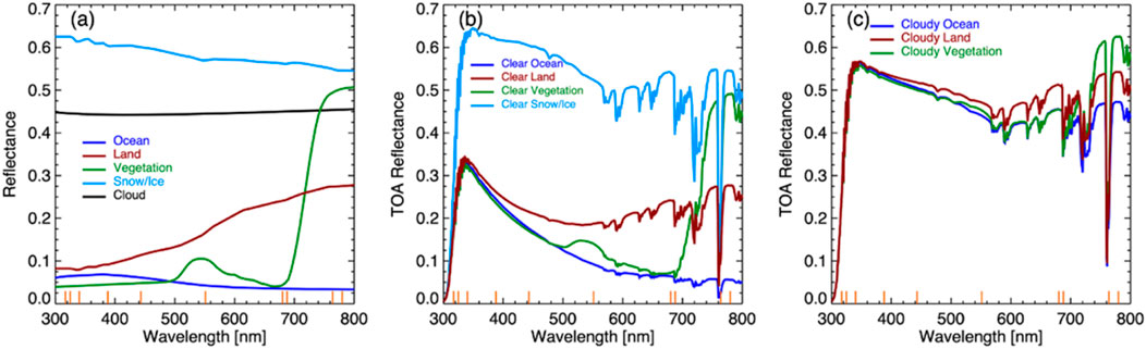
Figure 1. (a) Typical spectral reflectance of different reflector types without atmosphere; (b) TOA reflectance for clear atmosphere for different surfaces; (c) TOA reflectance for cloudy atmosphere with cloud optical depth of 10 for different surfaces. Solar zenith angle is 30° for all cases. 10 EPIC wavelength locations are indicated by orange ticks on x-axis.

Scattering from molecules and aerosols as well as absorption from gases can significantly modify the top-of-atmosphere (TOA) spectral reflectance (Figure 1b). The increase of spectral reflectance from 300 to 340 nm for all four surface types is mainly due to competition of ozone absorption and molecular Rayleigh scattering. As wavelength increases, molecular scattering cross section decreases, and the TOA reflectance resembles underlying surface reflectance except for some gas absorption features. In general, snow/ice is the brightest among four surface types. Land-ocean contrast (reflectance over land minus reflectance over ocean) is largest in the NIR channel and smallest in the UV/blue channels. Note that although vegetation in NIR is much larger than non-vegetation land, for global average, land-ocean (including vegetation and non-vegetation land) contrast is mainly governed by a non-vegetation land because green vegetation covers less than 5% of EPIC images (Wen et al., 2019).

TOA cloudy sky reflectance can be influenced by surface type. For a given cloud optical depth (COD) of 10, a brighter surface leads to a larger TOA reflectance. Clouds over land are brighter than clouds over ocean in visible and NIR wavelengths. Clouds over land are brighter than clouds over green vegetation for visible wavelengths, and less reflective in NIR. These relationships can be used to infer fundamental Earth observations in a quantitative manner.

Figure 2 shows EPIC natural color images taken at different times during a single day, demonstrating different features of the sunlit side of the Earth as it rotates about its axis. Near 0 UTC, almost the entire image is covered by the Pacific Ocean. As Earth rotates, the Eurasian continent appears near 6 UTC, followed by the African continent, the Atlantic Ocean, and America. Antarctica is bright and it is in the field-of-view (FOV) of EPIC all day in the Northern winter (the boreal winter) as Earth’s axis is tilted approximately 23.5° away from the Sun, contributing significantly to global average spectral reflectance.

Figure 2

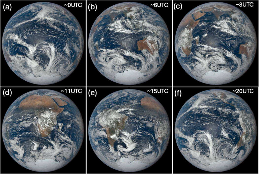
Figure 2. EPIC natural color images at different UTC time acquired on 1 January 2017. They demonstrate different features of the sunlit side of the Earth as it rotates about its axis. Note Figure (a) is centered over the Pacific Ocean; Figure (b,c) are centered over the Indian Ocean with Australia to the east and Africa to the west; Figure (d) is centered over the continent of Africa; Figure (e) is focused over the Atlantic Ocean and eastern South America and Figure (f) is centered over east Pacific with both North and South America visible. Antarctica is visible all day.

Figure 3 shows images of spectral reflectance in UV (388 nm), blue (443 nm), green (551 nm), red (680 nm) and NIR (780 nm) acquired on 1 January 2017 focused over the African continent and including parts of Antarctica. These images demonstrates that clouds are bright (more reflective) for all of these wavelengths. Land-ocean contrast is small for UV and blue bands as seen in Figures 3a,b. As wavelength increases, the land-ocean contrast increases. The African continent is somewhat visible in the green band (Figure 3c) but is bright in the red (Figure 3d) and even brighter in the NIR band (Figure 3f). Note that Antarctica is very bright in all wavelengths. As the Earth’s axis is tilted towards the Sun in the Northern summer (the boreal summer), EPIC sees more landmass, and the global average reflectance in red and NIR is expected to be larger compared to the boreal winter. Thus, the rotation of the Earth and the change of Earth’s tilt angle as the planet moves around the Sun bring about the variability of Earth’s spectral reflectance as well as reflected shortwave (SW) radiance and flux.

Figure 3

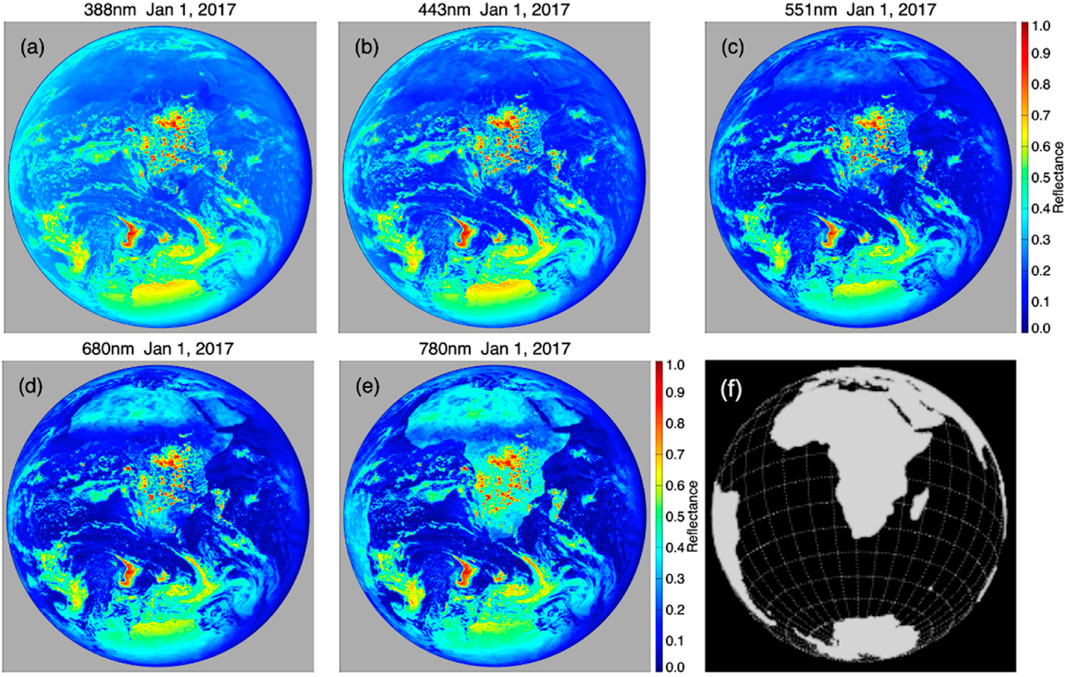
Figure 3. Five images (graphs (a–e)) of Earth taken on January 1, 2017, at different wavelengths: 388nm, 443nm, 551nm, 680nm, and 780nm, showing that (1) reflectance in UV and blue mainly influenced by clouds, (2) reflectance in longer wavelengths is impacted by both clouds and land surface, (3) Antarctica is bright in all five wavelengths. An additional black and white image in graph (f) displays a gridded map of Earth with continents in gray.

As EPIC is a major instrument on DSCOVR for monitoring the changes of planet Earth throughout its lifecycle, it is essential to understand the natural variabilities of EPIC observations on different time scales. In this paper, we quantify the variability of spectral reflectance and SW flux from EPIC and identify associated physical mechanisms. The data sets used in this study are described in Section 2, the analysis methods are described in Section 3, the results are presented in Section 4, and the summary and discussion are given in Section 5.

2 Data

In this paper, we analyze EPIC reflectance. Onboard the DSCOVR satellite, EPIC provides 10 narrowband spectral images of the entire sunlit face of Earth using a 2048 × 2048 pixel CCD (charge-coupled device) detector. EPIC’s 10 channels cover the spectral range from UV to NIR: 317, 325, 340, 388, 443, 552, 680, 688, 764, and 780 nm with filter width from 0.84 to 2.7 nm (see Table 1 in Herman et al., 2018). As the satellite orbits around the L₁ point, EPIC observes reflected solar radiation from the Earth in near backscatter directions. EPIC takes 13–22 images daily. The pixel size is about 8 km at nadir (angular resolution of 1.07 arc-second, Burt and Smith, 2012; Herman et al., 2018) with an effective resolution of 10 km when the point spread function is included. To maximize time cadence while reducing transmission time, the images of all wavelength channels, except 443 nm, have been reduced to 1,024 × 1,024 pixels (Herman et al., 2018; Marshak et al., 2018). The EPIC level-1 (L1B) data are analyzed for global average spectral reflectance for all 10 wavelengths.

Table 1

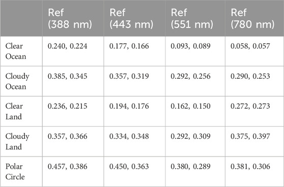
Table 1. Average spectral reflectance at 388, 443, 551, and 780 nm for different reflectors in January (blue color) and July (red color) 2017.

Cloud properties are retrieved by using reflectances at 388, 680, and 780 nm together with the two oxygen channels (Yang et al., 2018). The EPIC level-2 (L2) pixel-level cloud data include cloud mask, cloud optical depth, and cloud effective heights. Both EPIC L1B and L2 cloud data sets are publicly available at the NASA Langley data center.

The EPIC-based SW flux data are also analyzed. In the derivation of SW flux, narrowband-to-broadband regressions are applied to the EPIC measurements to derive the “EPIC broadband” reflectance for each EPIC pixel. The pixel-level broadband radiance is calculated from the reflectance, and the global mean SW radiance at each EPIC image time is obtained by simple average pixel-level SW radiance over the entire sunlit disk of the EPIC image of the Earth. The global daytime average SW flux is calculated using the EPIC-based broadband global mean broadband radiance and global anisotropic factor. The details of the algorithm is described in Su et al. (2018).

3 Analysis methods

We analyze EPIC-observed global average reflectance across all relevant wavelengths. The EPIC pixel-level reflectance is defined as

$r_{\lambda }=\frac{\pi I_{\lambda }}{F_{0,\lambda }}(1)$

where $I_{\lambda }$ is the EPIC measured radiance for a given pixel, and $F_{0,\lambda }$ is the TOA spectral solar irradiance at wavelength λ. In practice, the reflectance value ($r_{\lambda }$ in Equation 1) is calculated by multiplying the EPIC L1B data given in counts per second ($\text{count}·s^{-1}$) by the reflectance calibration factor. The reflectance calibration factors for EPIC channels are described by Herman et al. (2018) and Geogdzhayev and Marshak (2018) and can be found at the DSCOVR/EPIC website (https://epic.gsfc.nasa.gov/science/calibration/uv and https://epic.gsfc.nasa.gov/science/calibration/visnir).

Song et al. (2018) introduced a scattering function, $P_{\lambda }\left({\mathbf{\Omega }}_{\mathbf{0}},\mathbf{\Omega }\right)$, where ${\mathbf{\Omega }}_{\mathbf{0}}$ and $\mathbf{\Omega }$ is the direction of incidence (e.g., the Sun relative to the Earth) and scattering (e.g., the direction of DSCOVR spacecraft relative to the Earth), respectively. For EPIC images, the scattering phase function is estimated by the global average spectral reflectance of the planet Earth defined as

${\overline{R}}_{\lambda }\left({\mathbf{\Omega }}_{\mathbf{0}},\mathbf{\Omega }\right)=\frac{{\displaystyle {\sum }_{i=1}^N}{r}_{\lambda ,i}}{N}(2)$

where $r_{\lambda ,i}$ is the reflectance for ith pixel and N is the total number of pixels in an EPIC image. The near-hourly disk average reflectance for each EPIC image is further used to calculate the daily and monthly mean of the global spectral reflectance. Note that the simple average spectral reflectance is proportional to the average reflected spectral radiance (${\overline{I}}_{\lambda }\left({\mathbf{\Omega }}_{\mathbf{0}},\mathbf{\Omega }\right)$) towards EPIC as shown in Equation 3

${\overline{R}}_{\lambda }\left({\mathbf{\Omega }}_{\mathbf{0}},\mathbf{\Omega }\right)=\frac{{\pi \overline{I}}_{\lambda }\left({\mathbf{\Omega }}_{\mathbf{0}},\mathbf{\Omega }\right)}{F_{0,\lambda }}(3)$

As shown in Section 1, spectral reflectance differs dramatically over different surfaces (e.g., land, ocean, snow/ice) and is additionally influenced by the presence of clouds. To understand the variability of global average spectral reflectance, one needs to know the role of each reflector. We classify six reflector types. They are (1) clear ocean, (2) clear land, (3) cloudy ocean, (4) cloudy land outside of polar circles between −66.5° and +66.5°, (5) Antarctica (−90° to −66.5°) and (6) the Artic (66.5°–90°). We use the International Geosphere-Biosphere Programme (IGBP) map (Loveland and Belward, 1997) to distinguish land from ocean and EPIC L2 cloud mask data to determine whether a pixel is clear or cloudy.

In the EPIC cloud product, a pixel is classified as clear with high confidence, clear with low confidence, cloudy with low confidence, or cloudy with high confidence. Cloud fraction calculated using cloud mask with low or high confidence gives a global average cloud fraction of ∼65%, consistent with cloud fraction from GEO-LEO composite data sets (Yang et al., 2018; Delgado-Bonal et al., 2020). The same criterion is applied for cloud masking in this study. We also use CODs in the EPIC L2 cloud data. Without enough information to confidently determine cloud thermodynamic phase, two COD values are retrieved and reported for each cloudy pixel by assuming liquid and ice phases, respectively (Yang et al., 2018). Both COD values are used in this study to offer a range of physically observed results.

Unlike simple average for reflectance which is proportional to the global average radiance (Equation 2), surface area weighted average is needed for the global daytime average cloud fraction. Since each pixel in an EPIC image has the same angular resolution (1.07 arc-second) viewed from EPIC, or the same area ($\Delta s$) in the plane that is tangent the Earth and perpendicular to the Earth-spacecraft direction, the true area projected to the surface of the Earth is $\frac{\Delta s}{\cos \left(\theta \right)}$, where $\theta$ is the viewing angle. The global daytime average cloud fraction ($\overline{CF}$) is defined as

$\overline{CF}=\frac{{\displaystyle {\sum }_{i=1}^{N_c}}\frac{1}{\cos \left({\theta }_i\right)}}{{\displaystyle {\sum }_{j=1}^N}\frac{1}{\cos \left({\theta }_j\right)}}(\mathrm{4a})$

where $N_c$ and $N$ are number of cloudy pixels and total pixels in an EPIC image, respectively. The numerator is proportional to the area of clouds projected to the Earth surface, and the denominator is proportional to the daytime area of the Earth’s surface. Similarly, the area weighted average needed to calculate global daytime average COD ($\overline{\tau }$) is

$\overline{\tau }=\frac{{\displaystyle {\sum }_{i=1}^{N_c}}\frac{{\tau }_i}{\cos \left({\theta }_i\right)}}{{\displaystyle {\sum }_{i=1}^{N_c}}\frac{1}{\cos \left({\theta }_i\right)}}(\mathrm{4b})$

where ${\tau }_i$ is COD of ith pixel and $N_c$ is the total number of cloudy pixels in an EPIC image. We find that the simple pixel average underestimates annual mean cloud fraction by ∼3% and overestimates COD by ∼5% for both assumed liquid and ice clouds.

For an EPIC image, the global average reflectance can be expressed as a weighted sum of reflectance component from each reflector. Assuming that there are N pixels in an EPIC image and let N₁, N₂, N₃, … be pixels for type 1, 2, 3, … reflector components ($N={\sum }_i{N}_i$), then the sunlit disk average reflectance can be expressed as

$〈R〉=\frac{1}{N}\left[N_1\frac{{\displaystyle {\sum }_{i=1}^{N_1}}{r}_i}{N_1}+N_2\frac{{\displaystyle {\sum }_{i=1}^{N_2}}{r}_i}{N_2}+N_3\frac{{\displaystyle {\sum }_{i=1}^{N_3}}{r}_i}{N_3}+\dots \right]=f_1{R}_1+f_2{R}_2+f_3{R}_3+\dots (\mathrm{5a})$

where $r_i$ is the pixel-level reflectance, $f_j=\raisebox{1ex}{$N_j$}\!\left/ \!\raisebox{-1ex}{$N$}\right.$ and $R_j=\frac{{\displaystyle {\sum }_{i=1}^{N_j}}{r}_i}{N_j}$ is the fractional coverage and mean reflectance of $j^{th}$ reflector component in an EPIC image.

Each term on the right-hand side of Equation 5a is the reflectance component from corresponding reflector type to the global average reflectance. Equation 5a may be written as Equation 5b

$〈R〉=\sum L_j(\mathrm{5b})$

and

$L_j=R_j{f}_j(\mathrm{5c})$

where $L_j$ is the reflectance component from $j^{th}$ reflector to the global average reflectance. Note that $〈R〉$, $R_j$, f_j, and $L_j$ are determined from each EPIC image and are functions of time.

Figure 4 shows the reflectance component as a function of fractional coverage of each reflector type for January and July 2017, where each dot in the figure represents global average reflectance for one EPIC image. The reflectance component from each reflector is highly linearly correlated with the fractional coverage of that reflector in an EPIC image, as shown in Figure 4. We seek the best linear fit to the reflectance component vs. fractional coverage. We find that a straight line passing through the origin with the slope equal to the mean of average reflectances of m EPIC images (m dots in January 2017 in Figure 4) gives the best straight-line fit similar to the least-squares fit straight line passing through the origin by comparing the root-mean-square-error (RMSE) of the fits. Statistically, the reflectance component of $j^{th}$ reflector can be approximated as

${\overline{L}}_j={\overline{R}}_j{f}_j(\mathrm{6a})$

where ${\overline{R}}_j$ is the mean of the average reflectance of m EPIC images in the time period concerned (such as m dots in Figure 4 for January 2017). The linear relationship can be used to interpret the observed reflectance variability. Summing up reflectance component (Equation 6a) yields the global average reflectance

$\overline{〈R〉}={{\overline{R}}_{1}f}_1+{\overline{R}}_2{f}_2+{{\overline{R}}_{3}f}_3+\dots (\mathrm{6b})$

Figure 4

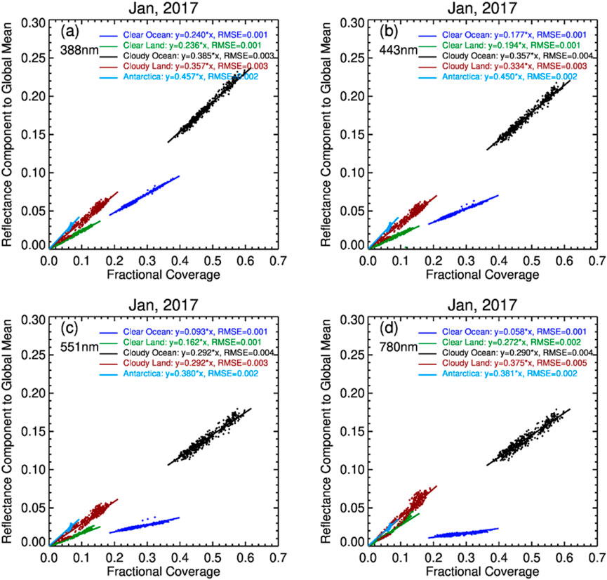
Figure 4. Four scatter plots show the relationship between fractional coverage (fj in Equation 5c) and the reflectance component (Lj in Equation 5c) to the global mean for different reflectors in January 2017. Each plot represents different wavelengths: (a) 388 nm, (b) 443 nm, (c) 551 nm, and (d) 780 nm. Scattered points depict data for clear ocean, clear land, cloudy ocean, cloudy land, and Antarctica. Linear equations with root mean square error (RMSE) values for each environment are provided in the legends, showing how reflectance varies with fractional coverage across different spectral bands.

Note that Wen et al. (2019) used a least-squares fit to estimate the relationship between fractional coverage and reflectance component from different reflectors. They found that the slope of the fit was equal to a weighted mean reflectance for each reflector. Here, the slope is simply the mean of the global reflectance from a series of EPIC images, such as monthly mean of global reflectance. The linear relations (Equations 6a, 6b) are used to interpret observations in Section 4.

Table 1 summarizes the average reflectance, or the slope of the linear fit, for UV, blue, green, and NIR bands for different reflectors for January (Figure 4) and July 2017, respectively. For clear and cloudy ocean, the average reflectance decreases with wavelength. For clear and cloudy land, the average reflectance decreases with wavelength from UV to green band, followed by an increase to the NIR band. There is a strong seasonal variation in average reflectance over cloudy ocean for all four wavelengths. From January to July, there is a strong decrease of ∼0.04 in average cloudy ocean reflectance for all four wavelengths (∼11% for UV and ∼15% for NIR band). Note the average reflectance of Antarctica (polar circle in January) is significantly larger than the average reflectance of the Arctic for all four wavelengths. This likely reflects the mixture of ice, melt ponds, open water and exposed land which can be observed in the Arctic while Antarctica is more homogeneous in snow and ice cover over land.

Because the slope of the linear fit is equal to the average reflectance of each reflector type, it can be used to understand the land-ocean contrast observable in Figure 3. For this discussion, the land-ocean contrast is defined as the difference between clear land and clear ocean average reflectance for a given wavelength. The observations clearly show that the average UV (388 nm) reflectance for clear land (0.236 in January, 0.215 in July) is almost the same as that for clear ocean (0.240 in January, 0.224 in July) resulting in a land-ocean contrast close to zero. This is in agreement with the unnoticeable land-ocean contrast in the UV channel (Figure 3). For the blue band at 443 nm, the land-ocean contrast is about 0.01–0.02, slightly larger than that for the UV band, and land and ocean become visible. As the wavelength increases, the difference between clear land and clear ocean average reflectance increases, resulting in an increase in land-ocean contrast. The land-ocean contrast of 0.214 for the NIR band at 780 nm is about three times as large as that (0.07) for the green band at 551 nm.

Because the Earth revolves around the Sun in an elliptical orbit and the incident of solar irradiance at the Earth varies as $D^{-2}$, where $D$ is the Earth-Sun distance in AU (Astronomical Unit), there is a ∼6.7% peak-to-peak change in incident solar irradiance over a year (Kopp et al., 2005; Kopp, 2023) and this variation consequently impacts the annual variation in reflected SW radiance and flux (Su et al., 2020). For a given Earth atmosphere system, a shorter Earth-Sun distance results in a larger incident solar irradiance, thus, a larger reflected SW radiance and flux compared to a larger Earth-Sun distance. However, the Earth’s SW albedo and broadband reflectance characteristics will remain the same. To correct the direct effect of Earth-Sun distance variation on the reflected SW radiance and flux variability, the SW radiance and flux are normalized to the mean Earth-Sun distance by multiplying $D^2$. The normalized SW radiance and flux are proportional to the broadband reflectance and albedo for incident of solar irradiance at mean Earth-Sun distance at 1 AU.

4 Results

EPIC global reflectance and EPIC-based SW radiance and flux are analyzed to characterize associated variabilities on different time scales. The relationships of global reflectance across EPIC wavelength channels are investigated as presented below.

First, we present the hourly variation of the global average spectral reflectance on a 24-h time scale in January (boreal winter) and July (boreal summer) in 2017 (Figure 5).

Figure 5

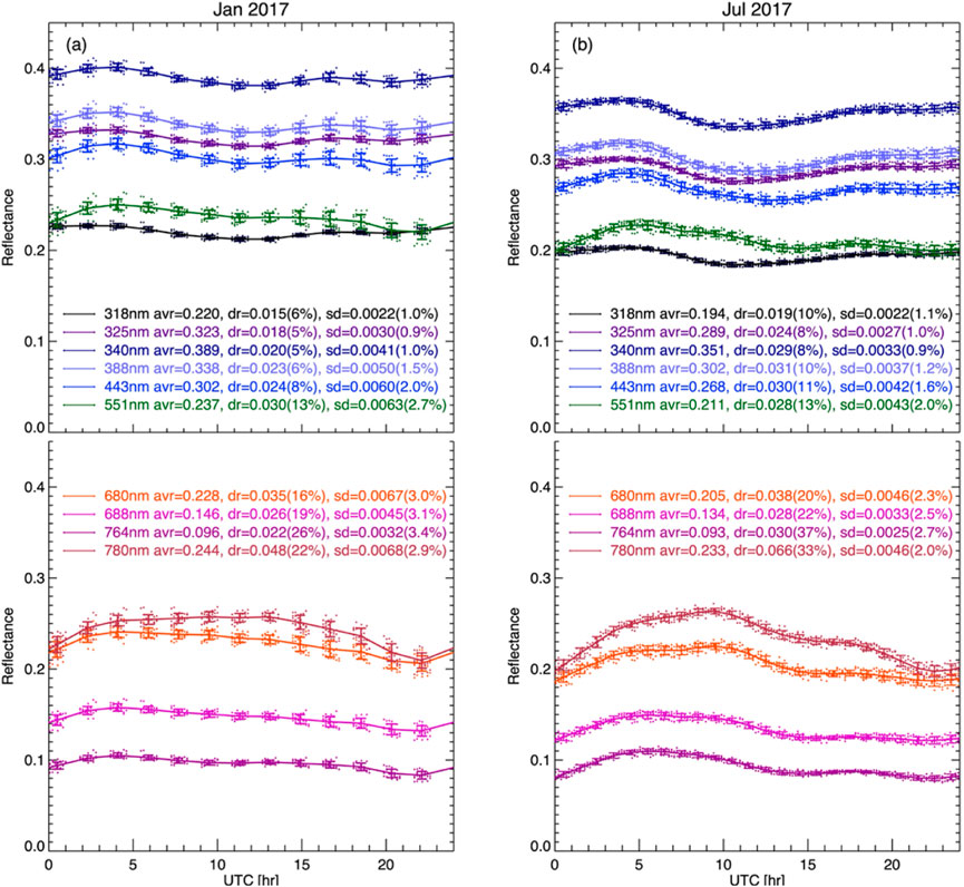
Figure 5. (a) shows hourly variation of global spectral reflectance for boreal winter (January 2017); (b) is similar to the (a) panel but for boreal summer (July 2017). Each dot represents the global average reflectance for one EPIC image. Solid lines are averages for the month. 24-h average (avr), and variation (dr = max-min) of average reflectance (solid line) with percent variation ((max-min)/min) are indicated. The average standard deviation (sd) of spectral reflectance and associated percent variation (average of sd/mean) of near-hourly data are also indicated.

There are ∼13 and ∼22 images taken by EPIC each day in January and July, respectively. For January, there are 13 clusters of spectral reflectance. Each cluster represents images taken at a similar UTC time during the month. For July, the observations are almost continuous because EPIC takes images almost hourly (every 65 min). Solid lines are fit through the average reflectance for each of 13 reflectance clusters for January and the average for each hour interval for July. Thus, the solid lines show the average variation of daytime spectral reflectance.

In the UV and blue bands, the global reflectance increases with wavelength, reaching a maximum at 340 nm, followed by a decrease towards blue wavelength at 443 nm. This is the result of competition of the decrease of the ozone absorption cross section in the Higgins bands and molecular scattering optical depth as wavelength increases. Reflectance in the UV and blue band, except stronger ozone absorbing 318 nm band, is significantly larger than reflectance in red and NIR. This is mainly due to much stronger molecular scattering in UV and blue bands compared to the red and NIR bands. The global average reflectance in the NIR band (780 nm) is significantly larger than the red band (680 nm) reflectance. The reflectance in the oxygen bands (A-band at 764 nm and B-band at 688 nm) is much smaller than the nearby reference with a minimum in the oxygen A-band among all 10 wavelength bands. The average green band (551 nm) reflectance is comparable with NIR reflectance in January and significantly smaller than NIR reflectance in July. The 24-h average reflectance is significantly larger in January than in July for all wavelengths.

The hourly variability of global reflectance depends on wavelength and season (e.g., January vs. July) (Figure 5). The hourly UV (all 4 UV bands) and blue reflectance vary with time like a sinusoidal function, increasing from 0 UTC reaching a maximum near 4-5 UTC, followed by a decrease to a minimum near 11–13 UTC with a subsequent increase reaching a local maximum near ∼16 UTC in January and ∼18 UTC in July, followed by a decrease towards 24 UTC for both January and July. The hourly reflectance of red and NIR bands varies similarly with time, increasing from 0 UTC, reaching a broad maximum near ∼10 UTC, followed by a decrease towards 24 UTC for both months, with a much more pronounced maximum for July. The reflectance of the green band and the two oxygen bands varies similarly with time, increasing from 0 UTC, reaching a broad maximum near ∼6 UTC, followed by a decrease towards 24 UTC for both January and July.

Figure 5 shows that the average 24-h variability is much larger in green (551 nm) and longer wavelengths compared to UV and blue bands and much larger in July than in January for all wavelength bands, both in the absolute value ($R_{\mathit{max}}-R_{\mathit{min}}$) and in the relative one ($\left(R_{\mathit{max}}-R_{\mathit{min}}\right)/R_{\mathit{min}}$). In January, the average 24-h variability is between ∼5% and ∼8% for the UV and blue bands and between ∼13% and ∼26% for longer wavelengths. In July, the average 24-h variability is ∼8%–∼11% for the UV and blue bands and ∼13%–∼37% for longer wavelengths. The NIR reflectance has the largest average 24-h variability among all wavelength bands.

The standard deviations within a 1-h interval in July and a ∼1.8-h interval in each of 13 observation groups in January are used to measure the variability of spectral reflectance for a given time-interval over the month. The standard deviations (the error bars in Figure 5) are significantly larger in January than in July. We found that the standard deviations of fractional coverage of cloudy ocean and cloudy land are comparable for both January and in July (not shown here). The main reason for a much larger standard deviation for “near-hourly” spectral reflectance in January is due to much larger average spectral reflectance in January compared to July for cloudy ocean, which makes the largest contribution to the global average reflectance (see Table 1). It is clear that for a given average cloudy ocean reflectance (${\overline{R}}_{cldocn}$) the change of the reflectance component of cloudy ocean (${\Delta \overline{L}}_{cldocn}$) due to the change of cloud fraction ($\Delta f_{cldocn}$) is ${\Delta \overline{L}}_{cldocn}={\overline{R}}_{cldocn}\Delta f_{cldocn}$. With similar variability in the fraction of cloudy ocean ($\Delta f_{cldocn}$) for both months, much larger variability of near-hourly reflectance in January is primarily due to much larger average reflectance of cloudy ocean compared to July. This suggests that the global daytime average COD in January is significantly larger than in July, as presented in Figure 9.

Because each component of spectral reflectance is linearly related to the fractional coverage (see Figure 4), the hourly variation of global average reflectance may be explained by the variation of fractional coverage of each reflector. The upper panels of Figure 6 show the average hourly variations of coverage of cloudy ocean, cloudy for both ocean and land, clear land, and cloudy (both land and ocean) and clear land for January (left) and July (right), respectively. The lower panels of Figure 6 show the average hourly global reflectance of UV, blue, and NIR bands for January (left) and July (right), respectively. The average global reflectances are calculated using the average variation of fractional coverage of different reflectors and associated average reflectance using Equation 6b. The calculated average reflectances resemble those from observations (Figure 5).

Figure 6

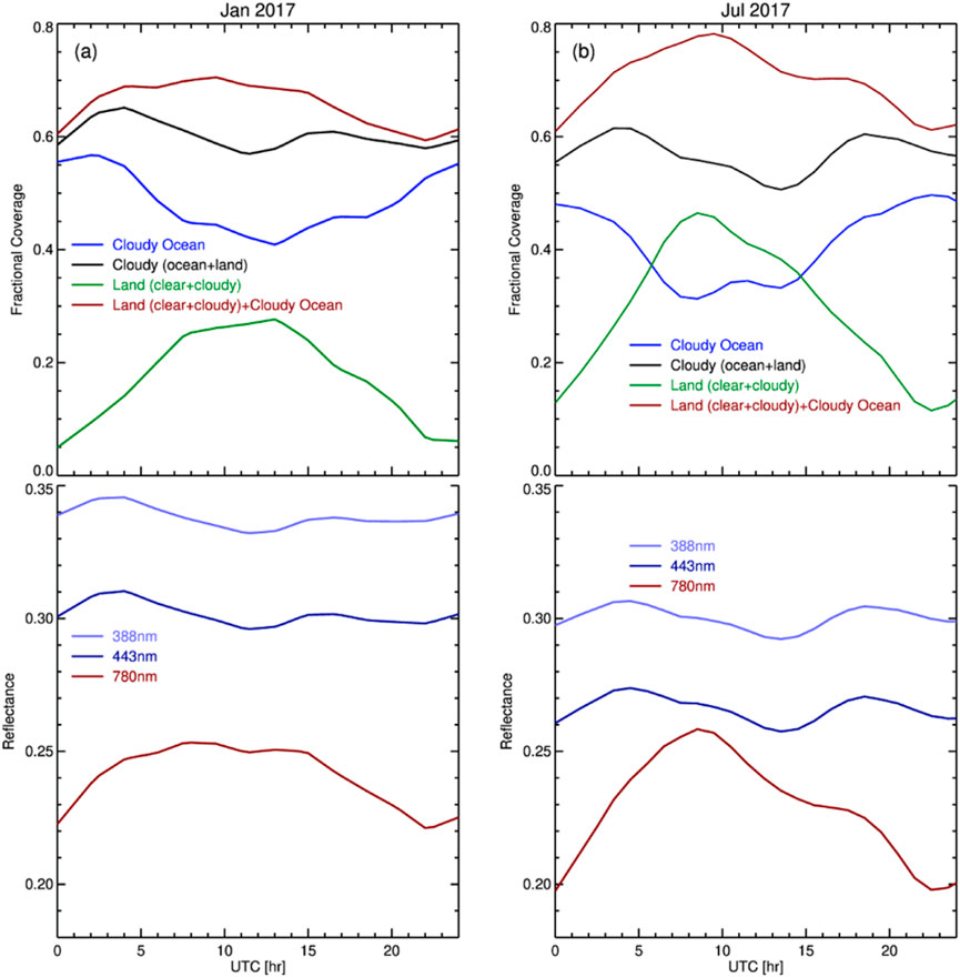
Figure 6. (a) The upper panel shows the hourly variations of average fractional coverage for cloudy ocean, cloudy for both land and ocean, land (both clear and cloudy), and land (clear and cloudy) plus cloudy ocean, and the lower panel show hourly variation of global spectral reflectance calculated from average fractional coverages (Equation 6b) for January 2017. (b) similar to (a) but for July 2017.

The following provides detailed analyses to interpret observations for January when Antarctica is in the field of view of EPIC and the Arctica is not in the sunlit side of the Earth. Similar analyses applicable to July observation are omitted for simplicity.

For the UV bands, the average reflectance for cloudy land is similar to that for cloudy ocean, and the average reflectance for clear land is similar to that for clear ocean (see Figures 1b,c). The global average reflectance in UV can be approximated by

$\overline{〈R〉}\approx {{\overline{R}}_{cloudy}f}_{cloudy}+{\overline{R}}_{clear}{f}_{clear}+{{\overline{R}}_{Ant}f}_{Ant}(\mathrm{7a})$

where ${\overline{R}}_{cloudy}$ is the average reflectance of clouds, ${\overline{R}}_{clear}$ is the average reflectance of clear region, ${\overline{R}}_{Ant}$ is the average reflectance of Antarctica, $f_{cloudy}$ is cloud fraction, $f_{clear}$ is the fraction of clear region, $f_{Ant}$ is the fraction of Antarctica in an EPIC image. In January, $f_{Ant}$ varies slowly with time (while in July $f_{Ant}=0$), and $f_{cloudy}+f_{clear}\approx const$ (since $f_{cloudy}+f_{clear}{+f}_{Ant}=1$ and $f_{Ant}\approx const$). Equation 7a becomes

$\overline{〈R〉}\approx \left({\overline{R}}_{cloudy}-{\overline{R}}_{clear}\right)f_{cloudy}+{\overline{R}}_{clear}const+{{\overline{R}}_{Ant}f}_{Ant}(\mathrm{7b})$

Thus, the hourly UV reflectance is approximately a linear function of cloud fraction ($f_{cloudy}$) (see Equation 7b). The sinusoidal variation of global average reflectance in the UV band is evidently a result of the similar sinusoidal variation of global daytime cloud coverage, both over the ocean and land (see black lines in the upper panels of Figure 6). To a large extent, the hourly variation of global cloud cover may also be used to explain the variation of the blue band reflectance.

For the NIR band, clouds and clear land are bright for both green vegetation and non-green vegetated land (e.g., desert and bare soil in Figures 1–3), while clear ocean is dark. The global average reflectance in NIR can be approximated by

$\overline{〈R〉}\approx {{\overline{R}}_{cld-ocean}f}_{cld-ocean}+{{\overline{R}}_{cld-land}f}_{cld-land}+{\overline{R}}_{clr-land}{f}_{clr-land}+{{\overline{R}}_{Ant}f}_{Ant}(\mathrm{8a})$

where ${\overline{R}}_{cld-ocean}$ , ${\overline{R}}_{cld-land}$ , ${\overline{R}}_{clr-land}$ ${\overline{R}}_{clr-land}$ is the average reflectance of cloudy ocean, cloudy land, and clear land, and $f_{cld-ocean}$, $f_{cld-land}$, $f_{clr-land}$ is associated fractional coverage, respectively. Here, the small reflectance component of the clear ocean is ignored. From Equation 8a, the average global reflectance is approximately the sum of three components, as

$\overline{〈R〉}\approx {{\overline{R}}_{cld}f}_{cld}+{\overline{R}}_{clr-land}{f}_{clr-land}+{{\overline{R}}_{Ant}f}_{Ant}(\mathrm{8b})$

where ${\overline{R}}_{cld}$, ${\overline{R}}_{clr-land}$ is the average reflectance of clouds and clear land, and $f_{cld}$, $f_{clr-land}$ is associated fractional coverage, respectively. Because the fraction of the Antarctica continent in the disk of the Earth in EPIC images varies slowly with time during a month, the variation of global average reflectance in NIR is mainly determined by the variation of global cloud fraction and clear land coverage (see Equation 8b).

The data show that fractional coverage of cloudy ocean is maximum near 0 UTC when the Pacific Ocean is in the middle of the EPIC image for both January and July (see Figure 2). As the Earth rotates, the fractional coverage of cloudy ocean decreases with time, reaching a broad minimum around ∼10–12 UTC, when the African continent is in the middle of the EPIC images, followed by an increase towards the original value at 24 UTC. Opposite to the variation of cloudy ocean coverage, the land fraction is minimum near 0 UTC. As the Earth rotates, EPIC starts seeing the Asian and Eurasian continents, and the land fraction reaches a maximum near ∼10 UTC when the African continent is in the middle of the EPIC images. Combining the two bright reflectors in NIR (cloud and land), the data show that the fractional coverage of the combination of the two bright reflectors is minimum at 0 UTC and increases with time, reaching a maximum near ∼10 UTC, followed by a decrease towards 24 UTC. Note that the rate of increase of the fractional coverage of the two bright reflectors is much faster in July than in January. This is because Earth’s axis of rotation tilts towards the Sun, and EPIC sees more Northern Hemisphere (N.H.), which contains significantly more landmass than the Southern Hemisphere (S.H.) (e.g., ∼68% of the Earth’s land in the N.H. vs. ∼32% in the S.H.). The same mechanism is responsible for the variation of spectral reflectance in the red band.

To validate the use of the variation of fractional coverages for interpreting the variation of corresponding global average spectral reflectance, their correlation coefficients are examined. Table 2 shows the correlation coefficients between the global average reflectance in the UV and blue bands and the global cloud fraction; it also highlights the correlation between reflectance in the NIR band and land fraction plus cloud fraction over ocean for both January and July. High correlation coefficients suggest that daytime variation of the global spectral reflectance can be explained by the variation of fractional coverage of relevant reflectors (i.e., cloud cover for UV/blue, land fraction (both clear and cloudy) plus cloud fraction over ocean for NIR).

Table 2

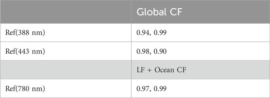
Table 2. Correlation coefficients between global average reflectance in the UV (Ref(388 nm)) and blue (Ref(443 nm)) bands and global cloud fraction (CF); and between reflectance in the NIR band (Ref(780 nm)) and land fraction (LF) plus ocean CF for January (blue color) and July (red color), 2017.

Because EPIC takes about 13 images per day in boreal winter and 22 images per day in boreal summer, different sampling size could affect the monthly averages. To answer this question, we have performed an analysis for EPIC observations in July 2017. Instead of using all 22 images of a day, we used every other image to calculate the monthly mean spectral reflectance. We found that the difference in monthly average spectral reflectance is insignificant whether the analyses are based on the original 22 images or sub-sampled 11 images. Thus, the sampling size of 13 or 22 does not have a significant impact on calculating the monthly average because the sampling size is large enough and the sampling time interval is close to being even such that major features of the Earth are captured by EPIC.

To understand the behavior of EPIC global spectral reflectance, it is useful to perform correlation analyses for all 10-channel reflectances. Using near-hourly global average spectral reflectances, the correlation matrices for any pair of EPIC spectral reflectances are clculated. The correlation matrices are presented in Figure 7a for January, April, July, and October of 2017 to represent Northern winter, spring, summer, and autumn. Figure 7a shows that there are two distinct wavelength groups in the matrices: the shorter wavelength group from 318 nm to 443 nm (UV and blue channels) and the longer wavelength group from 551 nm to 780 nm. Any pair of global average spectral reflectance within the same spectral group is highly correlated. However, any pair of global average spectral reflectance across the two spectral groups is poorly correlated.

Figure 7

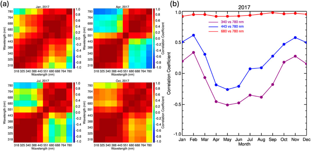
Figure 7. (a) Correlation matrices for EPIC global average reflectance across 10 wavelength bands for January, April, July, and October 2017; (b) seasonal variation of the correlation coefficients for selected pairs of wavelengths in 2017.

Figure 7b shows seasonal variation of the correlation coefficient between spectral reflectance of NIR (780 nm) and UV (340 nm), NIR and blue (443 nm), and NIR (780 nm) and red (680 nm). It is evident that reflectance in NIR is well correlated with red band reflectance, with correlation coefficients above ∼0.9 throughout the year. However, the NIR reflectance is poorly correlated with the UV and blue band reflectance. The NIR-blue correlation coefficient is slightly larger than the NIR-UV correlation coefficient. From January to February, there is a slight increase in correlation coefficient for both pairs of reflectance (i.e., NIR-blue and NIR-UV), followed by a strong decrease, reaching a minimum in May, then an increase from May to October, followed by a slight decrease from October to December.

Figure 7b shows seasonal variation of the correlation coefficient between spectral reflectance of NIR (780 nm) and UV (340 nm), NIR and blue (443 nm), and NIR (780 nm) and red (680 nm). The data show that reflectance in NIR is well correlated with red band reflectance, with correlation coefficients above ∼0.9 throughout the year. However, the NIR reflectance is poorly correlated with the UV and blue band reflectance. The NIR-blue correlation coefficient is slightly larger than the NIR-UV correlation coefficient. From January to February, there is a slight increase in correlation coefficient for both pairs of reflectance (i.e., NIR-blue and NIR-UV), followed by a strong decrease, reaching a minimum in May, then an increase from May to October, followed by a slight decrease from October to December.

As explained in Section 1, the land-ocean contrast is small for the UV and blue bands. The global average reflectance in UV and blue bands is primarily determined by global average cloud fraction. Thus, spectral reflectances in UV and blue bands are highly correlated. Reflectance in red and NIR bands is mainly determined by global average cloud fraction and clear land coverage. Thus, the reflectance in red is highly correlated with reflectance in NIR. Because land-ocean contrast in the green is significantly larger than in the UV and blue bands, and large land-ocean contrast at surface can significantly impact the TOA land-ocean contrast for the two oxygen bands, the reflectance in those bands is well correlated with the red and NIR bands compared to the UV and blue bands.

The variation of land cover viewed by EPIC explains the variability of the correlation coefficients between UV/blue and NIR bands. The daily average land fraction (excluding the polar circles) observed by EPIC increases from the minimum (∼0.18) in January to the maximum (∼0.32) in May, followed by a decrease towards December. The clear land fraction increases from the minimum (∼0.06) in January to the maximum (∼0.14) in May, followed by a decrease towards December. From minimum of 0.06 to maximum of 0.14, there is about a 130% ((max-min)/min) increase in clear land fraction. The cloudy land fraction follows the same trend as clear land fraction variation, with a minimum ∼0.12 in January and ∼0.18 in May, about a 50% increase in cloudy land fraction. Because the major difference between UV/blue and NIR reflectance comes from clear land, the minimum correlation coefficient between UV/blue and NIR is primarily due to the minimum clear land fraction in May as viewed by EPIC.

Near hourly EPIC global spectral reflectance is averaged to obtain the daily mean. The daily global reflectance data are analyzed below.

Figure 8 presents the daily variation of spectral reflectance in blue (443 nm) and NIR (780 nm) bands. The global average reflectance is decomposed into components from different reflectors (clear and cloudy ocean, clear and cloudy land, the Arctic and Antarctica) based on Equation 5a. The data clearly show that the variation of the reflectance component for each reflector type follows closely with the fractional coverage of each reflector type for both blue and NIR reflectance. There are two maxima in reflectance for both bands, a primary in December/January (peaked near December 16) and a secondary in May (peaked near May 20). The maxima are primarily caused by the presence of bright Antarctic and Arctic areas, respectively. There are two minima near March 30 and September 17, close to equinox day. The minima are primarily due to very small fraction of the polar regions in the sunlit side of the Earth near equinox days.

Figure 8

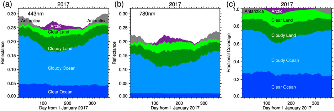
Figure 8. Three-panel graph showing data from 2017. Panel (a) displays daily mean reflectance and associated reflectance components at 443 nm, and panel (b) at 780 nm, both over days from January first. Reflectance components include those from clear and cloudy ocean, land, Arctic, and Antarctica. Panel (c) shows fractional coverage of associated reflectors. Each reflectance component and fractional coverage are color-coded: blue for water, green for land, purple for the Arctic, and gray for Antarctica.

In the December maximum, the reflectance component from Antarctica is ∼0.032 for the blue band and ∼0.027 for the NIR band, contributing ∼10% to the global reflectance for both bands. In the May maximum, the reflectance component from the Arctic is ∼0.028 for the blue band and ∼0.023 for the NIR, also contributing ∼10% to the global reflectance for both bands. Note that Antarctica is significantly brighter than the Arctic (Table 1). A similar percentage contribution of the two polar regions to the global reflectance is related to the fact that there are more clouds in boreal winter than summer, resulting in a larger average reflectance in the winter than in the summer, consequently a similar percentage contribution to the global reflectance from the two polar regions.

It is evident that presence of bright Antarctica and the Arctic surfaces on Earth and the Earth’s axial tilt change throughout a year cause the largest variation in spectral reflectance in a year. This phenomenon has been observed through CERES SW flux measurements (Loeb et al., 2007). Without the snow/ice covered polar regions, the variability of the global reflectance would be much smaller (see Figure 8).

As mentioned earlier, spectral reflectance for a given UTC time is more variable in boreal winter (January) than in boreal summer (July). The data show that the variability of cloud fraction for a given UTC time in boreal winter is similar to boreal summer (not shown here). However, the average spectral reflectance of cloudy ocean in boreal winter is found to be significantly larger than in boreal summer (see Table 1), suggesting significantly larger COD in January than in July.

The daily average of cloud fraction and CODs (both assuming liquid and ice phases) are presented in Figure 9. The daytime average cloud fraction decreases from ∼64% in January to a minimum in the middle of April, followed by an increase to the maximum of ∼67% in December. There is a large seasonal variation in daytime average CODs, both assuming liquid and ice phase. The COD, assuming liquid phase, decreases from ∼14 in January to ∼11 at the end of March, climbing up to ∼12 in the mid of June, dropping to ∼9 in early August, followed by an increase to ∼14 in December. The COD, assuming ice phase, varies in a similarly way as that assuming liquid phase. A significantly large average COD, consequently significantly a large average reflectance component from clouds, in boreal winter is likely the major cause of larger variability of spectral reflectance for a given UTC time (the standard deviation in Figure 5).

Figure 9

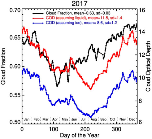
Figure 9. Line graph showing cloud fraction and cloud optical depth (COD) for 2017. Black line represents cloud fraction with a mean of 0.63 and standard deviation of 0.03. Red and blue lines represent COD, with means of 11.5 and 8.6, and standard deviations of 1.4 and 1.2, assuming liquid and ice respectively. The x-axis shows days of the year, and left y-axis and right y-axis display cloud fraction and COD values, respectively.

Monthly global average EPIC spectral reflectance data are calculated from the daily mean. The following provides analyses on monthly average data.

Monthly average EPIC spectral reflectances are presented in Figure 10. There are three important features in monthly average reflectance. First, there are two maxima in spectral reflectance in December/January and May, and two minima in April and September, except for ozone absorbing bands at 318 and 325 nm. Second, the reflectances are well correlated between any pairs of wavelengths. Third, the variability of monthly average reflectance throughout a year is much larger than the variability of 24-h variations in a day.

Figure 10

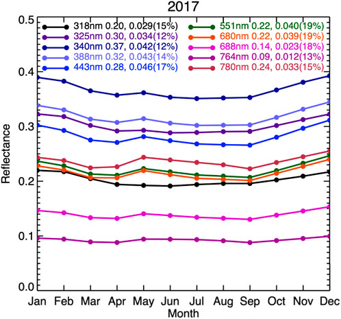
Figure 10. Monthly average EPIC global spectral reflectance. In the legend, the wavelength is followed by the annual mean, the annual variability (max-min), and percent variability [(max-min)/min] in the parenthesis.

For understanding the seasonal variation of the spectral reflectance, we examine the daily average reflectance and associated contribution from different reflector types in the blue and NIR bands (see Figure 8). The data show that there are two maxima (December/January and May) due to the presence of Antarctica and the Arctic in all spectral reflectance and two minima in April and September due to very small fraction of the snow/ice covered polar regions in the sunlit side of the Earth. These maxima and minima are the major cause of the seasonal variability of the EPIC spectral reflectances. It is interesting to note that the maximum in May for the NIR band is slightly higher than reflectance in January (though less than reflectance in December) because the land fraction also reaches its maximum in May (see Figure 11).

Figure 11

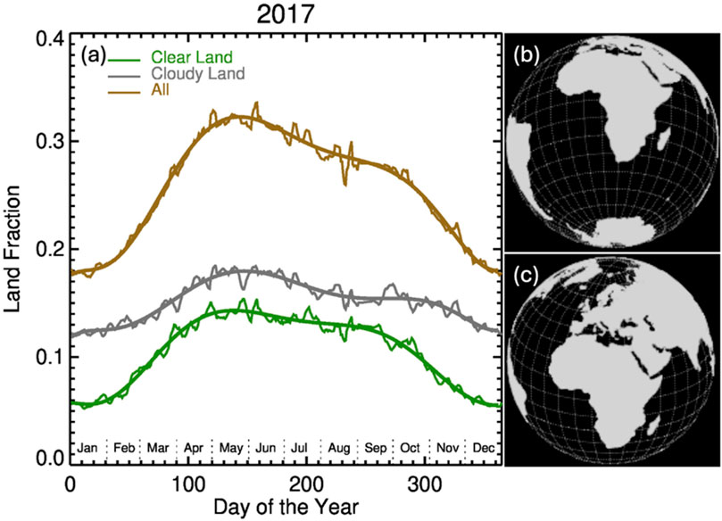
Figure 11. (a) shows the change of daily average land fraction, including clear and cloudy land and excluding polar circles, over a year (with months indicated); (b) demonstrates the sunlit side of the Earth at ∼11 UTC on 1 January 2017, showing continents of Africa, part of Eurasian and South America, and Antarctica in the FOV of EPIC; similar to (b) but on 10 May 2017 (c), and the Arctic is in the FOV of EPIC.

As mentioned in Section, Su et al. (2018) calculated SW radiance and flux based on EPIC observed narrow-band reflectance allowing us to quantify associated variabilities. The following presents analyses on EPIC-based SW radiance and flux.

Figure 12 presents examples of the global average sunlit side SW flux, SW radiance, and anisotropic factor. The global average anisotropic factor ($\overline{\rho }$) is defined as

$\overline{\rho }=\frac{\pi {\overline{I}}_{sw}}{{\overline{F}}_{sw}}(\mathrm{9a})$

where ${\overline{I}}_{sw}$ and ${\overline{F}}_{sw}$ are the daytime average SW radiance and flux, respectively (see Su et al., 2018). The daytime average SW flux can be obtained by

${\overline{F}}_{sw}=\frac{\pi {\overline{I}}_{sw}}{\overline{\rho }}(\mathrm{9b})$

Figure 12

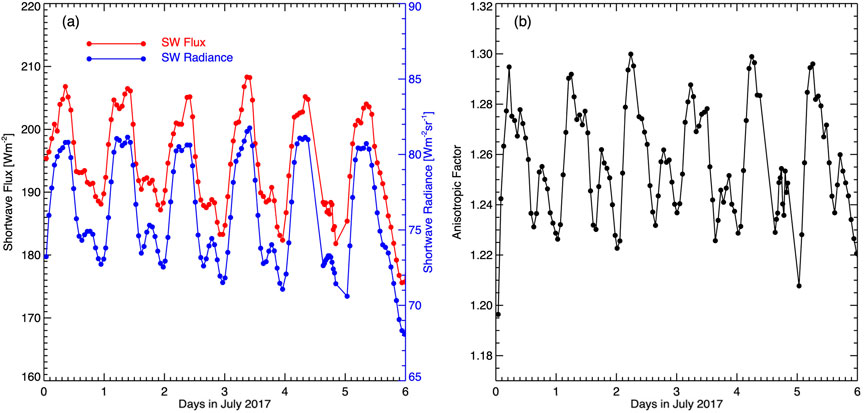
Figure 12. (a) EPIC-based global average broadband SW flux (red) and radiance (blue); (b) associated global average anisotropic factor.

The anisotropic factor is a measure for the degree of anisotropy of reflected SW radiation in terms of its angular dependence. For a Lambertian reflector, the reflected radiance field is isotropic (or angular independent), and the anisotropic factor is equal to unity.

Although Figure 12 only shows six-day observation in July 2017, a 24-h cycle is clear for SW radiance, SW flux, and anisotropic factor. In addition, Figure 13 shows hourly variation of SW flux, radiance, and anisotropic factor for January and July 2017 with EPIC images to demonstrate the position of continents and oceans at some specific UTC time. For January, starting from 0 UTC, SW flux and radiance increase with time, reaching a broad maximum ∼5 UTC, followed by a decrease towards 24 UTC. The average 24-h variability (max-min in the red line) is about 10% for both SW flux and radiance.

Figure 13

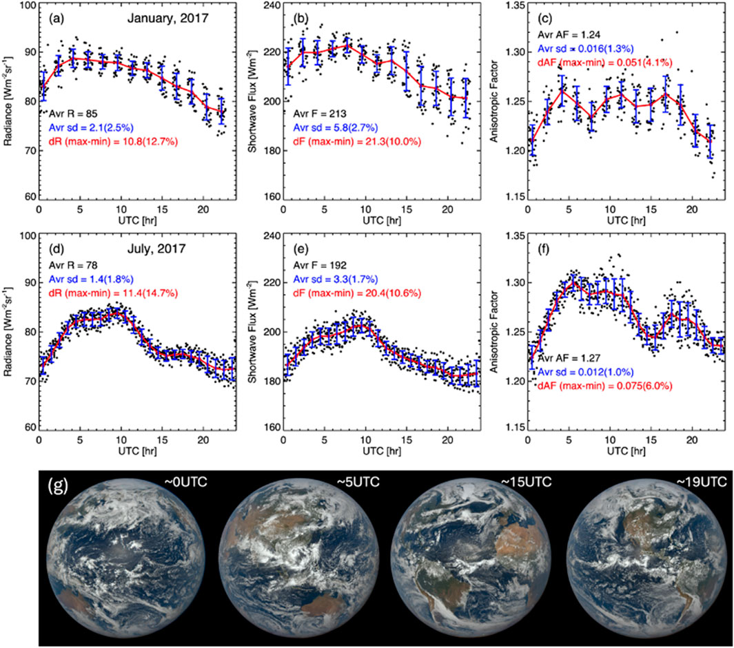
Figure 13. (a) 24-h variation of EPIC-based global broadband SW radiance, (b) broadband SW flux, (c) anisotropic factor for January 2017; (d–f) are similar to (a–c), but for July 2017; (g) EPIC images acquired on 16 July 2017.

The hourly variability of SW flux, radiance, and anisotropic factor changes with season. A broad maximum in SW radiance near ∼5–10 UTC is more pronounced in July compared to January. Similar to narrowband reflectance, SW radiance and flux are larger in January than in July. It is interesting to note that the anisotropic factor is smallest ∼0 UTC when the Pacific Ocean is in the middle of EPIC images, with a secondary minimum ∼15 UTC when the Atlantic Ocean is in the middle of EPIC images (see EPIC images in Figure 13). A broad maximum in anisotropic factor near ∼5–10 UTC is more pronounced for July. There is a local maximum in anisotropic factor near ∼19 UTC when the continent of America is in the middle of EPIC image. To summarize, the minimum anisotropic factor is associated with the Pacific Ocean and Atlantic Ocean is in the middle of the EPIC images, and maximum anisotropic factor is associated with the large landmass in the middle of the EPIC images.

The absolute variability (max-min) of the broadband SW radiance and flux in January is similar to that in July. The relative variability in January is slightly smaller than in July mainly because broadband SW radiance and flux are larger in January. Similar to narrowband reflectance, the variability of broadband SW radiance and flux measured by the standard deviation for a given time is significantly larger for January than July.

The anisotropic factor is ∼1.2–1.25 in January and ∼1.22–1.30 in July. Thus, the global average broadband SW radiance is highly anisotropic. For a Lambertian reflector ($\overline{\rho }=1$), the broadband SW flux is simply equal to $\pi {\overline{I}}_{sw}$. The assumption of a Lambertian reflector will overestimate the global SW flux by ∼20–30%.

Similar to the narrowband reflectance, the variability of broadband SW radiance and flux for a given UCT time, measured by the standard deviation, is significantly larger in January than in July. Again, this is likely due to a larger average reflectance in cloudy ocean in the boreal winter month than in the summer month, while the variability of cloud fraction is similar for the 2 months.

The monthly average SW flux and radiance data are presented in Figure 14. There are three important features in the monthly average SW flux and radiance. First, there are two maxima in SW flux and radiance, one in December/January and the another in May/June, and two minima, one in March/April and the other in August/September. Second, the May/June maximum for SW flux is significantly smaller than the December/January one compared to the SW radiance. Third, year-to-year variability of the monthly average SW flux is smaller than variability of SW radiance.

Figure 14

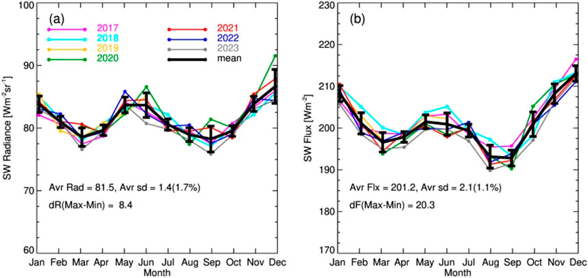
Figure 14. (a) Monthly mean of EPIC-based global SW radiance for 2017–2023; (b) like (a) but for SW flux. Seven-year average and standard deviation are presented in black color. The values of average SW radiance, flux, the average standard deviation about the seven-year monthly mean, and variability (max-min in black line) and are indicated.

The two maxima in EPIC-derived SW flux are similar to those observed by CERES albedo (Loeb et al., 2007). They are mainly due to the appearance of the bright Antarctica and Arctic regions on the sunlit side of the Earth. The larger variability in broadband SW radiance is primarily due to some occasions when the DSCOVR satellite was very close to the Sun-Earth line (the SEV angle reached only ∼2° in years 2020 and 2021), resulting in bright and wavelength dependence of sunlight reflected by water clouds (or the glory phenomenon) (Marshak, et al., 2021; Wen and Marshak, 2023).

The scattering angle effect can be seen from the relative variation of radiance to the mean. For SW radiance, the average variability (sd/avr) is ∼1.7%. For EPIC-derived SW flux, the average variability is ∼1%, significantly smaller than the relative variability for SW radiance, suggesting that the ADM model to convert SW radiance to flux has effectively accounted for those extreme situations when EPIC observations approached near-backscattering angles. This offers support to the work by Su et al. (2021).

5 Summary

EPIC global spectral reflectance and EPIC-derived SW radiance and flux offer tremendous insight into the Earth’s reflectance and associated variability on different time scales. Rotation of the Earth about its axis, uneven distribution of landmass, and wavelength dependence of different reflector types are the main cause for the variability of spectral reflectance on a 24-h time scale. The hourly variability of global average reflectance in red and NIR bands is much larger than the variation in UV and blue bands. The 24-h variability (max-min) in boreal summer (July) is larger (ranging from several percent larger in UV/blue bands to about 10% in NIR band) than in winter (January). For a given time, the variability of spectral reflectance is significantly larger in boreal winter than in summer. Based on near-hourly EPIC observations (22 images a day), we found that the global average reflectances are well correlated within the two wavelength groups: UV/blue and green/red/NIR, including two oxygen bands. Starting from January, the UV/blue and NIR correlation coefficient decreases with time, reaching a minimum in May followed by an increase to the maximum in December. This seasonal behavior is clearly due to the change of land fraction seen from EPIC as the direction of the Earth’s rotation axis varies throughout the year.

The data show that the presence of Antarctica and the Arctic is crucial for the daily averaged spectral reflectance variation throughout the year. Without snow/ice covered polar regions, the variability of daily average spectral reflectance would be much smaller. On a seasonal time scale, the variability of monthly average reflectance has similar variability across all 10 EPIC wavelengths mainly, due to the presence of Antarctica and the Arctic. This impact of the polar region of reflectance is critically important because this is not simply a reflection of which portions of the Earth are observed by EPIC, but it is a direct measurement of total radiation reflected back to space. Thus, these results are fundamental to understanding the seasonal energy balance of the Earth. As the Arctic and Antarctica may change (e.g., Kato et al., 2006; Weatherhead et al., 2010), these changes will also relevant to how this seasonal and multi-decadal energy balance may change.

The 24-h variability of SW radiance and flux in January are similar to that in July. The sunlit side average SW radiance is highly anisotropic. In the course of a day, the anisotropic factor varies from 1.2 to 1.27 in boreal winter and 1.22 to 1.30 in boreal summer, with a minimum when the Pacific Ocean is the center of the EPIC image and a maximum when the land (i.e., the Africa and Eurasian continents) is dominant in the EPIC image. The assumption of Lambertian reflection for SW radiance will overestimate the SW flux by 20%–30%. The seasonal variability of SW radiance and flux is mainly due to the presence of Antarctica and the Arctic regions. However, the variability of monthly average SW radiance is significantly larger than SW flux. This is because the change of scattering angle contributes in part to the variability of SW radiance but not to SW flux.

Over the past 10 years, DSCOVR/EPIC mission has been successfully proving near hourly multi-channel Earth images to inform global climate science. Algorithms have been developed to use EPIC observations to retrieve ozone and SO₂ amounts, aerosol and cloud optical depths and heights, and surface properties. 10 year’s worth of L2 and well calibrated L1 EPIC radiance datasets have been archived in NASA Langley Research Center Atmospheric Science Data Center (https://search.earthdata.nasa.gov/). DSCOVR/EPIC, together with other NASA missions (e.g., CERES, MODIS, VIIRS), will advance climate and atmospheric sciences in the years to come.

Data availability statement

The datasets presented in this study can be found in online repositories. The names of the repository/repositories and accession number(s) can be found below: https://epic.gsfc.nasa.gov/science/calibration/uv, https://epic.gsfc.nasa.gov/science/calibration/visnir, https://search.earthdata.nasa.gov/. EPIC natural color images can be downloaded from https://epic.gsfc.nasa.gov/.

Author contributions

GW: Conceptualization, Methodology, Writing – review and editing, Data curation, Writing – original draft, Investigation. AM: Conceptualization, Supervision, Writing – review and editing. WS: Data curation, Writing – review and editing. EW: Writing – review and editing.

Funding

The author(s) declare that no financial support was received for the research and/or publication of this article.

Acknowledgments

We are grateful to the DSCOVR science team for producing EPIC data products. The EPIC data were obtained from the NASA Langley Research Center Atmospheric Science Data Center.

Conflict of interest

The authors declare that the research was conducted in the absence of any commercial or financial relationships that could be construed as a potential conflict of interest.

The author(s) declared that they were an editorial board member of Frontiers, at the time of submission. This had no impact on the peer review process and the final decision.

Generative AI statement

The author(s) declare that no Generative AI was used in the creation of this manuscript.

Any alternative text (alt text) provided alongside figures in this article has been generated by Frontiers with the support of artificial intelligence and reasonable efforts have been made to ensure accuracy, including review by the authors wherever possible. If you identify any issues, please contact us.

Publisher’s note

All claims expressed in this article are solely those of the authors and do not necessarily represent those of their affiliated organizations, or those of the publisher, the editors and the reviewers. Any product that may be evaluated in this article, or claim that may be made by its manufacturer, is not guaranteed or endorsed by the publisher.

References

Burt, J., and Smith, B. (2012). “Deep space climate observatory: the DSCOVR mission,” IEEE Aerosp. Conf. Big Sky, 1–13. doi:10.1109/AERO.2012.6187025

CrossRef Full Text | Google Scholar

Carlson, B. E., Lacis, A. A., Russell, G. L., Marshak, A., and Su, W. (2022). Unique observational constraints on the seasonal and longitudinal variability of the Earth’s planetary albedo and cloud distribution inferred from EPIC measurements. Front. Remote Sens. 2, 788525. doi:10.3389/frsen.2021.788525

CrossRef Full Text | Google Scholar

Carn, S. A., Krotkov, N. A., Fisher, B. L., Li, C., and Prata, A. J. (2018). First observations of volcanic eruption clouds from the L1 Earth-Sun Lagrange point by DSCOVR/EPIC. Geophys. Res. Lett. 45. doi:10.1029/2018GL079808

CrossRef Full Text | Google Scholar

Davis, A., Ferlay, N., Libois, Q., Marshak, A., Yang, Y., and Min, Q. (2018). Cloud information content in EPIC/DSCOVR's oxygen A- and B-band channels: a physics-based approach. J. Quant. Spectrosc. Radiat. Transf. 220, 84–96. doi:10.1016/j.jqsrt.2018.09.006

CrossRef Full Text | Google Scholar

Delgado-Bonal, A., Marshak, A., Yang, Y., and L. Oreopoulos, L. (2020). Daytime variability of cloud fraction from DSCOVR/EPIC observations. J. Geophys. Res. Atmos., 125, e2019JD031488. doi:10.1029/2019JD031488

CrossRef Full Text | Google Scholar

Geogdzhayev, I. V., and Marshak, A. (2018). Calibration of the DSCOVR EPIC visible and NIR channels using MODIS Terra and Aqua data and EPIC lunar observations. Atmos. Meas. Tech. 11, 359–368. doi:10.5194/amt-11-359-2018

PubMed Abstract | CrossRef Full Text | Google Scholar

Herman, J., Huang, L., McPeters, R., Ziemke, J., Cede, A., and Blank, K. (2018). Synoptic ozone, cloud reflectivity, and erythemal irradiance from sunrise to sunset for the whole earth as viewed by the DSCOVR spacecraft from the earth–sun Lagrange 1 orbit. Atmos. Meas. Tech. 11, 177–194. doi:10.5194/amt-11-177-2018

CrossRef Full Text | Google Scholar

Jiang, J. H., Zhai, A. J., Herman, J., Zhai, C., Hu, R., Su, H., et al. (2018). Using deep space climate observatory measurements to study the earth as an exoplanet. Astron. J 156, 26. doi:10.3847/1538-3881/aac6e2

CrossRef Full Text | Google Scholar

Jin, Z., Charlock, T. P., Smith, Jr., W. L., and Rutledge, K. (2004). A parameterization of ocean surface albedo. Geophys. Res. Lett. 31, L22301. doi:10.1029/2004GL021180

CrossRef Full Text | Google Scholar

Kato, S., Loeb, N. G., Minnis, P., Francis, J. A., Charlock, T. P., Rutan, D. A., et al. (2006). Seasonal and interannual variations of top-of-atmosphere irradiance and cloud cover over polar regions derived from the CERES data set. Geophys. Res. Lett. 33 (19). doi:10.1029/2006GL026685

CrossRef Full Text | Google Scholar

Kopp, G. (2023). Daily solar flux as a function of latitude and time. Sol. Energy 249 (2023), 250–254. doi:10.1016/j.solener.2022.11.022

CrossRef Full Text | Google Scholar

Kopp, G., Heuerman, K., and Lawrence, G. (2005). The total irradiance monitor (TIM): instrument calibration. Sol. Phys. 230 (1), 111–127. doi:10.1007/s11207-005-7447-3

CrossRef Full Text | Google Scholar

Li, J., Fan, S., Kopparla, P., Liu, C., Jiang, J. H., Natraj, V., et al. (2019). Study of terrestrial glints based on DSCOVR observations. Earth Space Sci. 6, 166–173. doi:10.1029/2018EA000509

CrossRef Full Text | Google Scholar

Loeb, N. G., Wielicki, B. A., Rose, F. G., and Doelling, D. R. (2007). Variability in global top-of-atmosphere shortwave radiation between 2000 and 2005. Geophys. Res. Lett. 34, L03704. doi:10.1029/2006GL028196

CrossRef Full Text | Google Scholar

Loveland, T. R., and Belward, A. S. (1997). The IGBP-DIS global 1km land cover data set, DISCover: first results. Int. J. Remote Sens. 18 (15), 3289–3295. doi:10.1080/014311697217099

CrossRef Full Text | Google Scholar

Lu, Z., Wang, J., Chen, X., Zeng, J., Wang, Y., Xu, X., et al. (2023). First mapping of monthly and diurnal climatology of Saharan dust layer height over the Atlantic Ocean from EPIC/DSCOVR in deep space. Geophys. Res. Lett. 50, e2022GL102552. doi:10.1029/2022GL102552

CrossRef Full Text | Google Scholar

Lyapustin, A., Go, S., Korkin, S., Wang, Y., Torres, O., Jethva, H., et al. (2021). Retrievals of aerosol optical depth and spectral absorption from DSCOVR EPIC. Front. Remote Sens. 2, 645794. doi:10.3389/frsen.2021.645794

CrossRef Full Text | Google Scholar

Marshak, A., Varnai, T., and Kostinski, A. (2017). Terrestrial glint seen from deep space: oriented ice crystals detected from the Lagrangian point. Geophys. Res. Lett. 44, 5197–5202. doi:10.1002/2017GL073248

CrossRef Full Text | Google Scholar

Marshak, A., Herman, J., Szabo, A., Blank, K., Cede, A., Carn, S., et al. (2018). Earth observations from DSCOVR/EPIC instrument. Bull. Amer. Meteor. Soc. (BAMS) 9, 1829–1850. doi:10.1175/BAMS-D-17-0223.1

PubMed Abstract | CrossRef Full Text | Google Scholar

Marshak, A., Delgado-Bonal, A., and Knyazikhin, Y. (2021). Effect of scattering angle on earth reflectance. Front. Remote Sens. 2, 719610. doi:10.3389/frsen.2021.719610

CrossRef Full Text | Google Scholar

Ricchiazzi, P., Yang, S. R., Gautier, C., and Sowle, D.SBDART (1998). SBDART: a research and teaching Software Tool for plane-Parallel radiative Transfer in the Earth's atmosphere. Bull. Am. Meteorol. Soc. 79, 2101–2114. doi:10.1175/1520-0477(1998)079<2101:SARATS>2.0.CO;2

CrossRef Full Text | Google Scholar

Salomonson, V. V., Barnes, W. L., Maymon, P. W., Montgomery, H. E., and Ostrow, H. (1989). MODIS: advanced facility instrument for studies of the Earth as a system. IEEE Trans. geoscience remote Sens. 27 (2), 145–153. doi:10.1109/36.20292

CrossRef Full Text | Google Scholar

Salomonson, V. V., Barnes, W., and Masuoka, E. J. (2006). Introduction to MODIS and an overview of associated activities. Earth Sci. Satell. Remote Sens. 1, 12–32. doi:10.1007/978-3-540-37293-6_2

CrossRef Full Text | Google Scholar

Song, W., Knyazikhin, Y., Wen, G., Marshak, A., Mõttus, M., Yan, G., et al. (2018). Implications of whole-disc DSCOVR EPIC spectral observations for estimating Earth’s spectral reflectivity based on low-earth-orbiting and geostationary observations. Remote Sens. 10, 1594. doi:10.3390/rs10101594

CrossRef Full Text | Google Scholar

Su, W., Liang, L., Doelling, D. R., Minnis, P., Duda, D. P., Khlopenkov, K. V., et al. (2018). Determining the shortwave radiative flux from Earth polychromatic imaging camera. J. Geophys. Res. 123. doi:10.1029/2018JD029390

CrossRef Full Text | Google Scholar

Su, W., Minnis, P., Liang, L., Duda, D. P., Khlopenkov, K., Thieman, M. M., et al. (2020). Determining the daytime earth radiative flux from national Institute of standards and technology advanced radiometer (NISTAR) measurements. Atmos. Meas. Tech. 13 (2), 429–443. doi:10.5194/amt-13-429-2020

CrossRef Full Text | Google Scholar

Su, W., Liang, L., Duda, D. P., Khlopenkov, K., and Thieman, M. M. (2021). Global daytime mean shortwave flux consistency under varying EPIC viewing geometries. Front. Remote Sens. 2, 747859. doi:10.3389/frsen.2021.747859

CrossRef Full Text | Google Scholar

Weatherhead, E., Gearheard, S., and Barry, R. G. (2010). Changes in weather persistence: insight from Inuit knowledge. Glob. Environ. Change 20 (3), 523–528. doi:10.1016/j.gloenvcha.2010.02.002

CrossRef Full Text | Google Scholar

Wen, G., and Marshak, A. (2023). Effect of scattering angle on DSCOVR/EPIC observations. Front. Remote Sens. 4, 1188056. doi:10.3389/frsen.2023.1188056

CrossRef Full Text | Google Scholar

Wen, G., Marshak, A., Song, W., Knyazikhin, Y., Mõttus, M., and Wu, D. (2019). A relationship between blue and near-IR global spectral reflectance and the response of global average reflectance to change in cloud cover observed from EPIC. Earth Space Sci. 6 (8), 1416–1429. doi:10.1029/2019EA000664

CrossRef Full Text | Google Scholar

Wiscombe, W. J., and Warren, S. G. (1980). A model for the spectral albedo of snow. I: pure snow. J. Atmos. Sci. 37 (12), 2712–2733. doi:10.1175/1520-0469(1980)037<2712:amftsa>2.0.co;2

CrossRef Full Text | Google Scholar

Xiong, X., Che, N., and Barnes, W. (2005). Terra MODIS on-orbit spatial characterization and performance. IEEE Trans. Geoscience Remote Sens. 43 (2), 355–365. doi:10.1109/tgrs.2004.840643

CrossRef Full Text | Google Scholar

Xiong, X., Sun, J., Xie, X., Barnes, W. L., and Salomonson, V. V. (2009). On-orbit calibration and performance of Aqua MODIS reflective solar bands. IEEE Trans. Geoscience Remote Sens. 48 (1), 535–546. doi:10.1109/TGRS.2009.2024307

CrossRef Full Text | Google Scholar

Xu, X., Wang, J., Wang, Y., Zeng, J., Torres, O., Yang, Y., et al. (2017). Passive remote sensing of altitude and optical depth of dust plumes using the oxygen A and B bands: first results from EPIC/DSCOVR at Lagrange-1 point. Geophys. Res. Lett. 44, 7544–7554. doi:10.1002/2017GL073939

PubMed Abstract | CrossRef Full Text | Google Scholar

Yang, Y., Marshak, A., Mao, J., Lyapustin, A., and Herman, J. (2013). A method of retrieving cloud top height and cloud geometrical thickness with oxygen A and B bands for the deep space climate observatory (DSCOVR) mission: radiative Transfer simulations. J. Quant. Spectrosc. Radiat. Trans. 122, 141–149. doi:10.1016/j.jqsrt.2012.09.017

CrossRef Full Text | Google Scholar

Yang, W., Marshak, A., Várnai, T., and Knyazikhin, Y. (2018). EPIC spectral observations of variability in Earth’s global reflectance. Remote Sens. 10, 254. doi:10.3390/rs10020254

PubMed Abstract | CrossRef Full Text | Google Scholar